Third International Planetary Dunes Workshop (2012)
7039.pdf
SUPERVISED LEARNING STRATEGIES FOR AUTOMATED DETECTION OF MARTIAN DUNE FIELDS. L. Bandeira1, P. Pina1, J. S. Marques2 and J. Saraiva1, 1CERENA / IST (Av. Rovisco Pais, 1049-001 Lisboa, Portugal;
[email protected]), 2ISR / IST (Av. Rovisco Pais, 1049-001 Lisboa, Portugal).
Introduction: The knowledge on sand dunes on Mars has increased significantly with the availability of very high resolution (VHR) images of the surface, namely, MOC N/A and HiRISE [1]. Assessing the global distribution, shape and other characteristics of dunes with a higher detail can lead to an improved understanding of the interactions between the atmosphere and the surface of the planet [2]. The sheer quantity of data to be analyzed suggests that the use of automated methods can play an important role in fully exploiting the information that is being collected by automated probes. Thus, there are published studies using automatic procedures on temporal change detection [3, 4], determination of dune heights [5], morphologies [6] and spatial patterns [7], often considering analogies with terrestrial dunes. There is an automated method [8] using texture features and a neural network based classifier to identify terrestrial dunes on images with tens of meters but with performances below 70%. We have been addressing the development of automated methods for the delineation and characterization of dune fields, with good results on VHR images of Mars [9, 10]. In here, after a short reminder of our methodology, we report the most recent advances achieved. Methodology: The supervised learning strategy followed in our approach is based on the tiling of an image into relatively small square cells, which are then classified. These simple geometric shape makes the analysis very fast and leads to a non-iterative solution which is compatible with the large amount of data to be processed. This task is done through the extraction and analysis of local information (image features) along the regular grid of the tiled image. To benefit from context and diminish the dependence on specific factors such as illumination, an aggregation of the local features of neighbouring cells is performed within a block, i.e., a region constituted by 3×3 cells, and that constitutes the detection window of the methodology [11]. This block window is moved along the whole grid with a cell-sized step in order to analyse the complete image. For the mathematical formalism and additional details, consult our previous publication [10]. For this work we test the method with two different classifiers: Support-Vector Machine (SVM), as in previous works, and Random Forests (RF), that models the classification problem using multiple decision trees trained from random subsets of data [12].
Dataset: In order to demonstrate the generalized application of supervised learning strategies we continue to enlarge our dataset, now constituted by 230 MOC N/A images distributed around the surface of the planet. All have a spatial resolution better than 6.80 m/pixel, down to 1.45 m/pixel, in order to detect in detail small dune fields. About 70% of the images constituting the dataset (160 out of 230 images) include examples of the major types of dunes, according to the literature [13-15]: barchans (13%), barchanoid (19%), transverse (2%), dome (6%), linear (8%), star (1%), sand sheet (5%) and others (17%). These 160 images were visually analysed, in order to construct a ground-truth for each of them by manually drawing the contours of the dunes. The other 70 images (30% of the dataset) contain other geomorphological structures that can be confounded with dunes (channels, crater rims, textured terrain, among others). To compare the ground-truth with the result produced by the automated classifiers, both must be in the same format. Thus, we had to tile each groundtruth exactly like its corresponding original image. Furthermore, we had to consider three types of cells: ‘non-dune’, ‘dune’ and ‘unclassifiable’. To assign one of these labels to a cell, we computed the area occupied by dune terrain in the block from which it is the centre: if this area is less than 10% of the number of pixels of the block, the cell is ‘non-dune’; if it is higher than 30%, the cell is ‘dune’; if the area is between 10 and 30%, we decided not to classify it. Results: The performance of each classifier is evaluated through the computation of the probabilities = of false negatives ( pFN FN /( FN + TP ) ), false positives= ( pFP FP /( FP + TN ) ) and of a global error (
= perror pN . pFP + pP . pFN ), where FN stands for the number of false negative cells, TN the number of true negative cells, FP the number of false positive cells, TP the number of true positive cells, N the total number of negative cells and P the total number of positive cells. The classification output is illustrated globally in Fig. 1 on an entire MOC image and in detail in Fig. 2 on several images to illustrate successful and insuccessfull examples of the approach. The results we have obtained for the whole set of images confirm that this methodology is a valid contribution to the
Third International Planetary Dunes Workshop (2012)
automated mapping of dune fields on remotely sensed images. There are 370,019 cells to be classified in the 230 images, and the average global error obtained is 0.11. Moreover, we employed a cross-validation procedure where the dataset was divided in five groups, and each of those was used in turn to test the methodology (while the other four were, in each run, used for training). The five groups were built in such a way as to have a comparable number of positive ‘dune’ examples. The results for these five runs are similar and illustrate the robustness of the methodology: the lowest probability of error is 0.09, the highest is 0.14.
7039.pdf
SPA/110909). LB and JS acknowledge finantial support in the form of BPD and BD grants from FCT.
Table I – Classification performances. SVM RF
pFP 0.11 0.12
pFN 0.09 0.08
perror 0.11 0.10
We have also evaluated the classification performance by type of dune. Barchan and barchanoid types achieve the best performance with a probability of error of 0.09; on the other hand the star dunes, show the worst probability of error, but even this is only about 0.21, which we believe is due to a poor representation in the dataset. Conclusion: The performance of our methodology, based on gradient histograms coupled with either a SVM or a RF classifier, can be considered very good, with an average of error of about 11%. This fact reinforces the idea that advances made towards the classifiers may continue to lead to marginal gains in the detection of dune fields, indicating that the main area of future intervention should be on the extraction of other types of features combined with a multi-scale approach to better describe the whole pattern spectra of Martian dunes. References: [1] Bourke MC et al (2010) Geomorph, 121, 1-14. [2] Fenton LK and Hayward RK (2010) Geomorph, 121, 98-121. [3] Silvestro S et al (2010) GRL, 37, L20203. [5] Silvestro S et al (2011) GRL, 38, L20201, [5] Bourke MC et al (2006) Geomorph, 81, 440-452. [6] Ewing RC et al (2006) ESPL, 31, 1176-1191. [7] Bishop MA (2010) Geomorph, 120, 186-194. [8] Chowdhury PR et al (2011) IEEE JSTARS, 4, 171-184. [9] Bandeira L et al (2010) LNCS, 6112, 306-315. [10] Bandeira L et al (2011) IEEE GRSL, 8, 626-630. [11] Dalal N and Triggs B (2005) Proc. CVPR, 886-893. [12] Breiman L (2001) ML, 45, 5–32. [13] Mckee ED (1979) Univ. Press Pacific, Honolulu. [14] Hayward R et al (2007) JGR, 112, E1107. [15] Hayward R (2011) ESPL, 36(14), 1967-1972.
Acknowledgments: Work supported by FCT (Portugal), through project ANIMAR (PTDC/CTE-
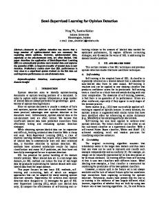
(a)
(b)
(c)
Fig. 1. Example of automated dune classification on E18-00494 image: (a) ground-truth; (b) SVM and (c) RF outputs (TP in green, TN in yellow, FN in red and FP in blue). [image credits: MSSS/NASA/JPL].
(a)
(b)
(c) (d) Fig. 2. Details of correct detections (a, b) and unsolved problems (c, d) in images differently zoomed (each cell is 40 pixels wide): (a) E03-02056. (b) R18-01147. (c) R17-02607. (d) E03-00618 (colours have the same meaning of Fig.1) [image credits: MSSS/NASA/JPL).