Support Tensor Machines for Text Categorization - CiteSeerX

Report No. UIUCDCS-R-2006-2714

UILU-ENG-2006-1746

Support Tensor Machines for Text Categorization

by Deng Cai, Xiaofei He, Ji-Rong Wen, Jiawei Han and Wei-Ying Ma

April 2006

Support Tensor Machines for Text Categorization∗ Deng Cai† †

Xiaofei He‡

Ji-Rong Wen∗

Jiawei Han†

Wei-Ying Ma∗

Department of Computer Science, University of Illinois at Urbana-Champaign ∗

Microsoft Research Asia Yahoo! Research Labs

‡

Abstract We consider the problem of text representation and categorization. Conventionally, a text document is represented by a vector in high dimensional space. Some learning algorithms are then applied in such a vector space for text categorization. Particularly, Support Vector Machine (SVM) has received a lot of attentions due to its effectiveness. In this paper, we propose a new classification algorithm called Support Tensor Machine (STM). STM uses Tensor Space Model to represent documents. It considers a document as the second order tensor in Rn1 ⊗ Rn2 , where Rn1 and Rn2 are two vector spaces. With tensor representation, the number of parameters estimated by STM is much less than the number of parameters estimated by SVM. Therefore, our algorithm is especially suitable for small sample cases. We compared our proposed algorithm with SVM for text categorization on two standard databases. Experimental results show the effectiveness of our algorithm.

1

INTRODUCTION

Text categorization is a task of assigning category labels to new documents based on a set of prelabelled documents. It is usually considered as a supervised or semi-supervised learning problem. During the last decade, a lot of learning algorithms have been proposed for text categorization, such as Support Vector Machines (SVM) [7], na¨ıve bayes [9], k-nearest neighbors and linear least square fit [19]. Most of these works are based on the Vector Space Model (VSM, [13]). The documents are represented as vectors, and each word corresponds to a dimension. The main reason of the popularity of VSM is probably due to the fact that most of the existing learning algorithms can only take vectors as their inputs, rather than tensors. ∗

The work was supported in part by the U.S. National Science Foundation NSF IIS-03-08215/IIS-05-13678. Any

opinions, findings, and conclusions or recommendations expressed in this paper are those of the authors and do not necessarily reflect the views of the funding agencies.

1

Support Vector Machines (SVM) is a relatively new learning approach introduced by Vapnik in 1995 for solving two-class pattern recognition problem [15]. It is based on the Structural Risk Minimization principle for which error-bound analysis has been theoretically motivated. The method is defined over a vector space where the problem is to find a decision surface that maximizes the margin between the data points in a training set. Previous investigations have demonstrate that SVM can be superior to other learning algorithms such as na¨ıve bayes [18]. In supervised learning settings with many input features, overfitting is usually a potential problem unless there is ample training data. For example, it is well known that for unregularized discriminative models fit via training-error minimization, sample complexity (i.e., the number of training examples needed to learn “well”) grows linearly with the Vapnik-Chernovenkis (VC) dimension. Further, the VC dimension for most models grows about linearly in the number of parameters [14], which typically grows at least linearly in the number of input features. All these reasons lead us to consider new representations and corresponding learning algorithms with less number of parameters. In this paper, we propose a novel supervised learning algorithm for text categorization, which is called Support Tensor Machine (STM). Different from most of previous text categorization algorithms which consider a document as a vector in Rn based on the vector space model, STM considers a document as a second order tensor in Rn1 ⊗ Rn2 , where n1 × n2 ≈ n. For example, a vector x ∈ Rn can be transformed by some means to a second order tensor X ∈ Rn1 ⊗ Rn2 .

A linear classifier in Rn can be represented as aT x + b in which there are n + 1 (≈ n1 × n2 + 1) parameters (b, ai , i = 1, · · · , n). Similarly, a linear classifier in the tensor space Rn ⊗ Rn can be

represented as uT Xv + b where u ∈ Rn1 and v ∈ Rn2 . Thus, there are only n1 + n2 + 1 parameters.

This property makes STM especially suitable for small sample cases.

Recently there has been a lot of interests in tensor based approaches to data analysis in high dimensional spaces. Vasilescu and Terzopoulos have proposed a novel face representation algroithm called Tensorface [16]. Tensorface represents the set of face images by a higher-order tensor and extends Singular Value Decomposition (SVD) to higher-order tensor data. Some other researchers have also shown how to extend Principal Component Analysis, Linear Discriminant Analysis, and Locality Preserving Projection to higher order tensor data [2],[6],[20]. Most of previous tensor based learning algorithms are focused on dimensionality reduction. In this paper, we extend SVM based idea to tensor data for classification. It is worthwhile to highlight several aspects of the proposed approach here: • While traditional linear classification algorithms like SVM find a classifier in Rn , STM finds a classifier in tensor space Rn1 ⊗ Rn2 . This leads to structured classification.

• The computation of STM is very simple. It can be obtained by solving two quadratic op-

timization problems. For each single optimization problem, the computational complexity √ approximately scales with n, where n is the dimensionality of the document space. There 2

are few parameters that are independently estimated, so performance in small data sets is very good. • This paper is primarily focused on the second order tensors. However, the algorithm and the analysis presented here can also be applied to higher order tensors.

The rest of this paper is organized as follows: Section 2 provides a brief description of the algebra of tensors and SVM. In Section 3, we give some descriptions on tensor space model for document representation. The Support Tensor Machine (STM) approach for text categorization is described in Section 4. In Section 5, we give a theoretical justification of STM and its connections to SVM. The experimental results on text databases are presented in Section 6. Finally, we provide some concluding remarks and suggestions for future work in Section 7.

2

PRELIMINARY

In this section, we provide a brief overview of the algebra of tensors and Support Vector Machine. For a detailed treatment please see [8], [15].

2.1

The Algebra of Tensors

A tensor with order k is a real-valued multilinear function on k vector spaces: T : Rn1 × · · · × Rnk → R The number k is called the order of T . A multilinear function is linear as a function of each variable separately. The set of all k-tensors on Rni , i = 1, · · · , k, denoted by T k , is a vector space under the

usual operations of pointwise addition and scalar multiplication:

(aT )(a1 , · · · , ak ) = a (T (a1 , · · · , ak )) , (T + T ′ )(a1 , · · · , ak ) = T (a1 , · · · , ak ) + T ′ (a1 , · · · , ak ) where ai ∈ Rni . Given two tensors S ∈ T k and T ∈ T l , define a map: S ⊗ T : Rn1 × · · · × Rnk+l → R by S ⊗ T (a1 , · · · , ak+l ) = S(a1 , · · · , ak )T (ak+1 , · · · , ak+l ) It is immediate from the multilinearity of S and T that S ⊗ T depends linearly on each argument

ai separately, so it is a (k + l)-tensor, called the tensor product of S and T .

For the first order tensors, they are simply the covectors on Rn1 . That is, T 1 = Rn1 , where Rn1

is the dual space of Rn1 . The second order tensor space is a product of two first order tensor spaces, 3

i.e. T 2 = Rn1 ⊗ Rn2 . Let e1 , · · · , en1 be the standard basis of Rn1 , and ε1 , · · · , εn1 be the dual

basis of Rn1 which is formed by coordinate functions with respect to the basis of Rn1 . Likewise, let e e1 , · · · , e en2 be a basis of Rn2 , and εe1 , · · · , εen2 be the dual basis of Rn2 . We have, εi (ej ) = δij and εei (e ej ) = δij

where δij is the kronecker delta function. Thus, {εi ⊗ εej } (1 ≤ i ≤ n1 , 1 ≤ j ≤ n2 ) forms a basis of

Rn1 ⊗ Rn2 . For any 2-tensor T , we can write it as: T =

X

1≤i≤n1 1≤j≤n2

Tij εi ⊗ εej

This shows that every 2-tensor in Rn1 ⊗ Rn2 uniquely corresponds to a n1 × n2 matrix. Given two P 1 P 2 vectors a = nk=1 ak ek ∈ Rn1 and b = nl=1 bl e el ∈ Rn2 , we have T (a, b) =

X ij

=

X

=

X

n2 n1 X X bl e el ) ak ek , Tij εi ⊗ εej ( k=1

n1 X

Tij εi (

ij

l=1 n 2 X

ak ek )e εj (

k=1

l=1

bl e el )

Tij ai bj

ij

= aT T b Note that, in this paper our primary interest is focused on the second order tensors. However, the algebra presented here and the algorithm presented in the next section can also be applied to higher order tensors.

2.2

Support Vector Machine

Support Vector Machines are a family of pattern classification algorithms developed by Vapnik [15] and collaborators. SVM training algorithms are based on the idea of structural risk minimization rather than empirical risk minimization, and give rise to new ways of training polynomial, neural network, and radial basis function (RBF) classifiers. SVM has proven to be effective for many classification tasks [7][12]. We shall consider SVMs in the binary classification setting. Assume that we have a data set D = {xi , yi }m i=1 of labeled examples, where yi ∈ {−1, 1}, and we wish to select, among the infinite

number of linear classifiers that separate the data, one that minimizes the generalization error, or at least minimizes an upper bound on it. It is shown that the hyperplane with this property is the one that leaves the maximum margin between the two classes. The discriminant hyperplane can be defined as f (x) = wT x + b 4

(1)

where w is a vector orthogonal to the hyperplane. Computing the best hyperplane is posed as a constrained optimization problem and solved using quadratic programming techniques. The optimization problem of SVM can be stated as follows: m

X 1 T ξi w w+C 2

min w,b,ξ

i=1

subject to

T

yi (w xi + b) ≥ 1 − ξi , ξi ≥ 0,

(2)

i = 1, · · · , m.

Given a new data point x to classify, a label is assigned according to its relationship to the decision boundary, and the corresponding decision function is g(x) = sign wT x + b

3




(3)

TENSOR SPACE MODEL

Document indexing and representation has been a fundamental problem in information retrieval for many years. Most of previous works are based on the Vector Space Model (VSM, [13]). The documents are represented as vectors, and each word corresponds to a dimension. In this section, we introduce a new Tensor Space Model (TSM) for document representation. In Tensor Space Model, a document is represented as a tensor. Each element in the tensor corresponds to a feature (word in our case). For a document x ∈ Rn , we can convert it to the

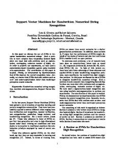
second order tensor (or matrix) X ∈ Rn1 ×n2 , where n1 × n2 ≈ n. Figure 1 shows an example of

converting a vector to a tensor. There are two issues about converting a vector to a tensor.

The first one is how to choose the size of the tensor, i.e., how to select n1 and n2 . In figure 1, we present two possible tensors for a 9-dimensional vector. Suppose n1 ≥ n2 , in order to have at least

n entries in the tensor while minimizing the size of the tensor, we have (n1 − 1) × n2 < n ≤ n1 × n2 .

With such requirement, there are still many choices of n1 and n2 , especially when n is large. Generally all these (n1 , n2 ) combinations can be used. However, it is worth noticing that the number of parameters of a linear function in the tensor space is n1 + n2 . Therefore, one may try to minimize n1 + n2 . In other words, n1 and n2 should be as close as possible. The second issue is how to sort the features in the tensor. In vector space model, we implicitly assume that the features are independent. A linear function in vector space can be written as g(x) = wT x. Clearly, the change of the order of the features has no impact on the function learning. In tensor space model, a linear function can be written as f (X) = uT Xv. Thus, the independency assumption of the features no longer holds for the learning algorithms in the tensor space model. Different feature sorting will lead to different learning result in the tensor space model. 5

1

1 4 7

2

2 5 8 3 6 9

3 Vector to Tensor Conversion

4 5

(a) 1 6

6

2 7

7

3 8

8

4 9

9

5 x (b)

Figure 1: Vector to tensor conversion. 1∼9 denote the positions in the vector and tensor formats. (a) and (b) are two possible tensors. The ‘x’ in tensor (b) is a padding constant.

In this paper, we empirically sort the features (words) according to their document frequency and then convert the vector into a n1 × n2 tensor such that n2 = 50. The better ways of converting

a document vector to a document tensor with theoretical guarantee will be left for our future work.

4

SUPPORT TENSOR MACHINES

4.1

The Problem

Given a set of training samples {Xi , yi }, i = 1, · · · , m, where Xi is the data point in order-2 tensor

space, Xi ∈ Rn1 ⊗ Rn2 and yi ∈ {−1, 1} is the label associated with Xi . Find a tensor classifier

f (X) = uT Xv + b such that the two classes can be separated with maximum margin.

4.2

The Algorithm

STM is a tensor generalization of SVM. The algorithmic procedure is formally stated below: 1. Initialization: Let u = (1, · · · , 1)T . 2. Computing v: Let xi = XTi u and β1 = kuk2 , v can be computed by solving the following optimization problem:

m

min v,b,ξ

X 1 ξi β1 vT v + C 2 i=1

subject to

yi (vT xi + b) ≥ 1 − ξi , ξi ≥ 0,

(4)

i = 1, · · · , m.

Note: The optimization problem (4) is the same as (2) in the standard SVM algorithm. Thus, any computational method for SVM can also be used here.

6

˜ i = Xi v and β2 = kvk2 . u can be computed by 3. Computing u: Once v is obtained, let x solving the following optimization problem:

m

X 1 ξi β2 uT u + C 2

min u,b,ξ

i=1

T

˜ i + b) ≥ 1 − ξi , yi (u x

subject to

ξi ≥ 0,

(5)

i = 1, · · · , m.

Note: As above, the optimization problem (5) is the same as (2) in the standard SVM algorithm and we can use the computational methods for SVM to solve (5). 4. Iteratively computing u and v: By step 2 and 3, we can iteratively compute u and v until they tend to converge. Note: The convergence proof is given in Section 5.2.

5

JUSTIFICATIONS

In this section, we provide a justification of our STM algorithm.

5.1

Large Margin Classifier in Tensor Space

Suppose we have a set of order-2 tensors X1 , · · · , Xm ∈ Rn1 ⊗ Rn2 . A linear classifier in the tensor

space can be naturally represented as follows:


f (X) = sign uT Xv + b ,

u ∈ Rn1 , v ∈ Rn2

Equation (6) can be rewritten through matrix inner product as follows:
f (X) = sign < X, uvT > +b , u ∈ Rn1 , v ∈ Rn2

(6)

(7)

Thus, the optimization problem in the tensor space is reduced to the following: m

min u,v,b,ξ

X 1 ξi kuvT k2 + C 2 i=1

subject to

T

yi (u Xi v + b) ≥ 1 − ξi , ξi ≥ 0,

(8)

i = 1, · · · , m.

We will now switch to a Lagrangian formulation of the problem. We introduce positive Lagrange multipliers αi , µi , i = 1, · · · , m, one for each of the inequality constraints (8). This gives Lagrangian: X X
1 kuvT k2 + C ξi − αi yi uT Xi v + b LP = 2 i i X X X + αi − αi ξi − µi ξi i

i

i

7

Note that
1 trace uvT vuT 2
1 T
v v trace uuT 2 1 T
T
v v u u 2

1 kuvT k2 = 2 = = Thus, we have: LP

=

X X
1 T
T
v v u u +C ξi − αi yi uT Xi v + b 2 i i X X X + αi − αi ξi − µi ξi i

i

i

Requiring that the gradient of LP with respect to u, v, b and ξi vanish give the conditions: P αi yi Xi v u= i T v v P αi yi uT Xi v= i T u u X αi yi = 0

(9) (10) (11)

i

C − αi − µi = 0,

i = 1, · · · , m

(12)

From Equations (9) and (10), we see that u and v are dependent on each other, and can not be solved independently. In the following, we describe a simple yet effective computational method to solve this optimization problem. We first fix u. Let β1 = kuk2 and xi = XTi u. Thus, the optimization problem (8) can be

rewritten as follows:

m

min v,b,ξ

X 1 ξi β1 kvk2 + C 2 i=1

subject to

yi (vT xi + b) ≥ 1 − ξi , ξi ≥ 0,

(13)

i = 1, · · · , m.

It is clear that the new optimization problem (13) is identical to the standard SVM optimization problem. Thus, we can use the same computational methods of SVM to solve (13), such as [5][10][11]. ˜ i = Xv. Thus, u can be obtained by solving the Once v is obtained, let β2 = kvk2 and x

following optimization problem:

m

min u,b,ξ

X 1 ξi β2 kuk2 + C 2 i=1

subject to

T

˜ i + b) ≥ 1 − ξi , yi (u x ξi ≥ 0, 8

i = 1, · · · , m.

(14)

Table 1: 41 semantic categories from Reuters-21578 used in our experiments category

ModeApte Train

Test

earn

2673

1040

acq

1435

crude trade

category

ModeApte Train

Test

ipi

27

9

620

nat-gas

22

11

223

98

veg-oil

19

11

225

73

tin

17

10

money-fx

176

69

cotton

15

9

interest

140

57

bop

15

8

ship

107

35

wpi

12

8

sugar

90

24

pet-chem

13

6

coffee

89

21

livestock

13

5

gold

70

20

gas

10

8

money-supply

70

17

orange

12

6

gnp

49

14

retail

15

1

cpi

45

15

strategic-metal

9

6

cocoa

41

12

housing

13

1

alum

29

16

zinc

8

4

grain

38

7

lumber

7

4

copper

31

13

fuel

4

7

jobs

32

10

carcass

6

5

reserves

30

8

heat

6

4

rubber

29

9

lei

8

2

iron-steel

26

11

Again, we can use the standard SVM computational methods to solve this optimization problem. Thus, v and u can be obtained by iteratively solving the optimization problems (13) and (14). In our experiments, u is initially set to the vector of all ones. By comparing the optimization problems of SVM (2) and STM (8), also noting that Xi in (8) is converted from xi in (2) through the “vector-to-tensor” conversion described in Section 3, STM can be thought of as a special case of SVM with the following constraint: wn1 (j−1)+i = ui vj

(15)

For n-dimensional documents, the w in decision function of SVM is also n-dimensional, so there are n + 1 (≈ n1 × n2 + 1) parameters for SVM. For STM, there are only n1 + n2 + 1 parameters.

Therefore, STM is much more computationally tractable and especially suitable for small sample cases.

9

5.2

Convergence Proof

In this section, we provide a convergence proof of the iterative computational method described above. We have the following theorem: Theorem 1 The iterative procedure to solve the optimization problems (13) and (14) will monotonically decreases the objective function value in (8), and hence the STM algorithm converges. Proof Define:

m

X 1 ξi f (u, v) = kuvT k2 + C 2 i=1

Let u0 be the initial value. Fixing u0 , we get v0 by solving the optimization problem (13). Likewise, fixing v0 , we get u1 by solving the optimization problem (14). Notice that the optimization problem of SVM is convex, so the solution of SVM is globally optimum [1][4]. Specifically, the solutions of equations (13) and (14) are globally optimum. Thus, we have: f (u0 , v0 ) ≥ f (u1 , v0 ) Finally, we get: f (u0 , v0 ) ≥ f (u1 , v0 ) ≥ f (u1 , v1 ) ≥ f (u2 , v1 ) ≥ · · · Since f is bounded from below by 0, it converges.

5.3

From Matrix to High Order Tensor

The STM algorithm described above takes order-2 tensors, i.e., matrices, as input data. However, the algorithm can also be extended to high order tensors. In this section, we briefly describe the STM algorithm for high order tensors. Let (Ti , yi ), i = 1, · · · , m denote the training samples, where Ti ∈ Rn1 ⊗ · · · ⊗ Rnk . The decision

function of STM is:

f (T ) = T (a1 , a2 , · · · , ak ) + b a1 ∈ Rn1 , a2 ∈ Rn2 , · · · , ak ∈ Rnk where T (a1 , a2 , · · · , ak ) =

X 1 ≤ i1 ≤ n1 . . . 1 ≤ ik ≤ nk

Ti1 ,··· ,ik a1i1 × · · · × akik

As before, a1 , · · · , ak can also be computed iteratively. We first introduce the l-mode product of a tensor T and a vector a, which we denote as T ×l a.

The result of l-mode product of a tensor T ∈ Rn1 ⊗ · · · ⊗ Rnk and a vector a ∈ Rnl , 1 ≤ l ≤ k will 10

Table 2: 56 semantic categories from TDT2 used in our experiments category

doc

category

num

doc

category

num

doc num

20001

1844

20087

98

20007

28

20015

1828

20096

76

20041

28

20002

1222

20021

74

20064

28

20013

811

20026

72

20089

25

20070

441

20008

71

20034

25

20044

407

20056

66

20004

21

20076

272

20037

65

20063

19

20071

238

20065

63

20043

18

20012

226

20005

58

20083

17

20023

167

20074

56

20078

16

20048

160

20009

52

20072

13

20033

145

20091

51

20029

13

20039

141

20031

49

20093

12

20086

140

20024

47

20084

12

20032

131

20042

35

20028

12

20047

123

20020

34

20050

11

20019

123

20011

33

20085

10

20077

120

20022

31

20053

10

20018

104

20017

29

be a new tensor B ∈ Rn1 ⊗ · · · ⊗ Rnl−1 ⊗ Rnl+1 ⊗ · · · Rnk , where Bi1 ,··· ,il−1 ,il+1 ,··· ,ik =

nl X il =1

Ti1 ,··· ,il−1 ,il ,il+1 ,··· ,ik · ail

Thus, the decision function in higher order tensor space can also be written as: f (T ) = T ×1 a1 ×2 a2 · · · ×k ak + b The optimization problem of STM in high order tensors is: m

min

a1 ,··· ,ak ,b,ξ

subject to

X 1 1 ka ⊗ · · · ⊗ ak k2 + C ξi 2

(16)

i=1

yi (Ti (a1 , a2 , · · · , ak ) + b) ≥ 1 − ξi , ξi ≥ 0,

i = 1, · · · , m.

Here ka1 ⊗ · · · ⊗ ak k denotes the tensor norm of a1 ⊗ · · · ⊗ ak [8].

First, to compute a1 , we fix a2 , · · · , ak . Let β2 = ka2 k2 , · · · , βk = kak k2 . We then define 11

Table 3: Performance comparison on Reuters-21578 Train&Test split

Method

micro F1

macro F1

SVM

.8490

.3355

STM

.8666

.4818

SVM

.8841

.4553

10% Train

STM

.8908

.5735

30% Train

SVM STM

.9225 .9196

.6618 .7357

50% Train

SVM STM

.9355 .9282

.7247 .7826

ModApte

SVM STM

.9368 .9321

.7356 .7877

5% Train

Table 4: Statistical significance tests on Reuters-21578 Train&Test split

sysA

sysB

s-test

S-test

T-test

5% Train

STM

SVM

10% Train

STM

SVM

≫

≫

≫

30% Train

STM

SVM


” or “ 0.05

≫ ≫ ≫

ti = Ti ×2 a2 · · · ×k ak . Thus, the optimization problem (16) can be reduced as follows: m

min

a1 ,b,ξ

subject to

X 1 β2 · · · βk ka1 k2 + C ξi 2 i=1

yi (a

1T

ti + b) ≥ 1 − ξi ,

ξi ≥ 0,

(17)

i = 1, · · · , m.

Again, we can use the standard SVM computational methods to solve this optimization problem. Once a1 is computed, we can fix a1 , a3 , · · · , ak to compute a2 . So on, all the ai can be computed

in such iterative manner.

6

EXPERIMENTS

In this section, several experiments were performed to show the effectiveness of our proposed algorithm. Two standard document collections were used in our experiments: Reuters-21578 and TDT2. We compared our proposed algorithm with Support Vector Machines. 12

6.1

Data Corpora

Reuters-21578 corpus1 contains 21578 documents in 135 categories. The ModApte version of Reuters-21578 is used in our experiments. Those documents with multiple category labels are discarded, and the categories with more than 10 documents are kept. It left us with 8213 documents in 41 categories as described in Table 1. For ModeApte split, there are 5899 training documents and 2314 testing documents. After preprocessing, this corpus contains 18933 distinct terms. The TDT2 corpus2 consists of data collected during the first half of 1998 and taken from six sources, including two newswires (APW, NYT), two radio programs (VOA, PRI) and two television programs (CNN, ABC). It consists of 11201 on-topic documents which are classified into 96 semantic categories. In this dataset, we also removed those documents appearing in two or more categories and use the categories which contain more than 10 documents thus leaving us with 10021 documents in 56 categories as described in Table 2. After preprocessing, this corpus contains 36771 distinct terms. Each document is represented as a term-frequency vector and each document vector is normalized to 1. We simply removed the stop words, and no further preprocessing was done. For STM, we empirically sort the features (words) according to their document frequency and then convert the vector into a n1 × n2 tensor such that n2 = 50.

6.2

Evaluation Metric

The classification performance is evaluated by comparing the predicted label of each testing document with that provided by the document corpus. The standard recall, precision and F1 measure are used here [17]. Recall is defined to be the ratio of correct assignments by the classifier divided by the total number of correct assignments. Precision is the ratio of correct assignments by the classifier divided by the total number of the classifier’s assignments. The F1 measure combines recall (r) and precision (p) with an equal weight in the following form: F1 (r, p) =

2rp r+p

These scores can be computed for the binary decisions on each individual category first and then be averaged over categories. Or, they can be computed globally over all the n × m binary decisions

where n is the number of total test documents, and m is the number of categories in consideration. The former way is called macro-averaging and the latter way is called micro-averaging. It is understood that the micro-averaged scores tend to be dominated by the classifier’s performance on common categories, and the macro-averaged scores are more influenced by the performance on rare categories. Providing both kinds of scores is more informative than providing either alone. 1 2

Reuters-21578 corpus is at http://www.daviddlewis.com/resources/testcollections/reuters21578/ Nist Topic Detection and Tracking corpus is at http://www.nist.gov/speech/tests/tdt/tdt98/index.html

13

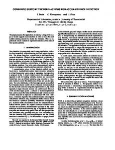
0.94 0.93 0.92

Micro F1

0.91 0.9 0.89 0.88 0.87

STM SVM

0.86 0.85 0.84

5% 10%

30%

50%

ModApte

Training sample ratio

Figure 2: Micro-averaged F1 on Reuters-21578 0.8 0.75 0.7

Macro F1

0.65 0.6 0.55 0.5 0.45

STM SVM

0.4 0.35 0.3

5% 10%

30%

50%

ModApte

Training sample ratio

Figure 3: Macro-averaged F1 on Reuters-21578

We also use a set of significance tests for comparing two classification methods with various performance measures. These significance tests are: • Micro sign test (s-test): A sign test designed for comparing two systems, A and B, based on their decisions on all the document/category pairs.

• Macro sign test (S-test): A sign test for comparing two systems, A and B, using the paired F1 values for individual categories.

• Macro t-test (T-test): A t-test for comparing two systems, A and B, using the paired F1 values for individual categories.

For more details about these significance tests, please refer to [18].

6.3

Experimental Results

We used the LIBSVM system [3] and tested it with the linear model, since previous researches [18] show that linear SVM is effective enough for text categorization. The dataset was randomly split into training and testing sets. In order to examine the effectiveness of the proposed algorithm with different size of the training set, we ran several tests that the 14

Table 5: Performance comparison on TDT2 Train&Test split

Method

micro F1

macro F1

SVM

.8881

.6477

STM

.9064

.7507

SVM

.9292

.7692

10% Train

STM

.9343

.8317

30% Train

SVM STM

.9602 .9563

.9063 .9152

50% Train

SVM STM

.9684 .9640

.9307 .9402

5% Train

Table 6: Statistical significance tests on TDT2 Train&Test split

sysA

sysB

s-test

S-test

T-test

5% Train

STM

SVM

10% Train

STM

SVM

≫

≫

≫

30% Train

STM

SVM

50% Train

STM

SVM

≪

∼

∼

≫ ≪

≫ >

≫ >

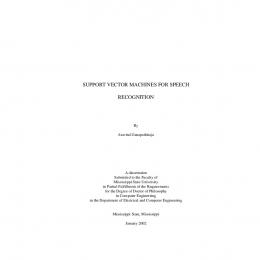
training set contains 5%, 10%, 30% and 50% documents, for both Reuters-21578 and TDT2. In all these splits, we kept at least two documents in every category of the training set. For each test, we averaged the results over 10 random splits. Moreover, for Reuters-21578 dataset, we also tested on the ModApte split which contains around 70% training sample. Table 3 and 5 show the classification results on two datasets. Table 4 and 6 summarized the statistical significance tests. Figure (2,3,4,5) show the performance with respect to the training set size. As can be seen from the above results, when the training set is small (5% and 10%), STM outperforms SVM on both micro-averaged F1 and macro-averaged F1 . As the number of training samples increases, STM performed better than SVM on macro-averaged F1 but worse on microaveraged F1 . As we know, the micro-level measure is dominated by the performance of the classifiers on large categories, while the macro-level measure is more sensitive to the performance of the classifiers on small categories [18]. The experimental results show the greater performance of STM on small training sample cases over SVM. To get a more detailed picture of the performance difference between STM and SVM over different size of training samples, we plot the performance curves of STM and SVM over different categories in Figure 6 and 7. The categories are sorted by the number of training samples. For those categories with the same number of training samples, we averaged their F1 scores. We can

15

0.97 0.96 0.95

Micro F1

0.94 0.93 0.92 0.91

STM SVM

0.9 0.89 0.88

5% 10%

30%

50%

Training sample ratio

Figure 4: Micro-averaged F1 on TDT2 dataset 1 0.95

Macro F1

0.9 0.85 0.8 0.75 0.7

STM SVM

0.65 0.6

5% 10%

30%

50%

Training sample ratio

Figure 5: Macro-averaged F1 on TDT2 dataset

see that STM is better than SVM on the left side of the figures (corresponding to small training set) but worse than SVM on the right side of the figures. This observation indicates that our STM algorithm is especially suitable for small sample problems. This is due to the fact that the number of parameters need to be estimated in STM is n1 +n2 +1 which can be much smaller than n1 ×n2 +1

in SVM.

7

Conclusions

In this paper we have introduced a tensor framework for document representation and classification. In particular, we have proposed a new classification algorithm called Support Tensor Machines (STM) for learning a linear classifier in tensor space. Our experimental results on Reuters-21578 and TDT2 databases demonstrate that STM is especially suitable for small sample cases. This is due to the fact that the number of parameters estimated by STM is much less than that estimated by standard SVM. There are several interesting problems that we are going to explore in the future work: 1. In this paper, we empirically construct the tensor. The better ways of converting a document vector to a document tensor with theoretical guarantee need to be studied. 16

1 1 0.9 0.9 0.8

Macro F1

Macro F1

0.8 0.7 0.6

0.7 0.6

0.5 STM SVM

0.5 STM SVM

0.4 0.4 0.3

1

10

2

10 Number of training samples per category

3

10

0.3

1

10 Number of training samples per category

Figure 6: Performance curves of all categories

2

10

Figure 7: Performance curves of all categories

on Reuters-21578 dataset (30% training sam-

on TDT2 dataset (10% training samples case)

ples case)

2. STM is a linear method. Thus, it fails to discover the nonlinear structure of the data space. It remains unclear how to generalized our algorithm to nonlinear case. A possible way of nonlinear generalization is to use kernel techniques. 3. In this paper, we use a iterative computational method for solving the optimization problem of STM. We expect that there exists more efficient computational methods.

References [1] Christopher J. C. Burges. A tutorial on support vector machines for pattern recognition. Data Mining and Knowledge Discovery, 2(2):121–167, 1998. [2] Deng Cai, Xiaofei He, and Jiawei Han. Subspace learning based on tensor analysis. Technical report, Computer Science Department, UIUC, UIUCDCS-R-2005-2572, May, 2005. [3] Chih-Chung Chang and Chih-Jen Lin. LIBSVM: a library for support vector machines, 2001. Software available at http://www.csie.ntu.edu.tw/~cjlin/libsvm. [4] R. Fletcher. Practical methods of optimization. John Wiley and Sons, 2nd edition edition, 1987. [5] Hans Peter Graf, Eric Cosatto, L´eon Bottou, Igor Dourdanovic, and Vladimir Vapnik. Parallel support vector machines: The cascade SVM. In Advances in Neural Information Processing Systems 17, 2004. [6] Xiaofei He, Deng Cai, and Partha Niyogi. Tensor subspace analysis. In Advances in Neural Information Processing Systems 18, 2005. 17

[7] Thorsten Joachims. Text categorization with support vector machines: Learning with many relevant features. In ECML’98, 1998. [8] John M. Lee. Introduction to Smooth Manifolds. Springer-Verlag New York, 2002. [9] A. McCallum and K. Nigam. A comparison of event models for naive bayes text classification. In AAAI-98 Workshop on Learning for Text Categorization, 1998. [10] John Platt. Using sparseness and analytic qp to speed training of support vector machines. In Advances in Neural Information Processing Systems 11, 1998. [11] John C. Platt. Fast training of support vector machines using sequential minimal optimization, pages 185–208. MIT Press, Cambridge, MA, USA, 1999. [12] R. Ronfard, C. Schmid, and B. Triggs. Learning to parse pictures of people. In ECCV’02, 2002. [13] Gerard Salton, A. Wong, and C. S. Yang. A vector space model for information retrieval. Communications of the ACM, 18(11):613–620, 1975. [14] V. N. Vapnik. Estimation of dependences based on empirical data. Springer-Verlag, 1982. [15] V. N. Vapnik. The Nature of Statistical Learning Theory. Springer-Verlag, 1995. [16] M. A. O. Vasilescu and D. Terzopoulos. Multilinear subspace analysis for image ensembles. In IEEE Conference on Computer Vision and Pattern Recognition, 2003. [17] Yiming Yang. An evaluation of statistical approaches to text categorization. Jounal of Information Retrieval, 1(1/2):67–88, 1999. [18] Yiming Yang and Xin Liu. A re-examination of text categoriztion methods. In SIGIR’99, 1999. [19] Yiming Yang, Jian Zhang, and Bryan Kisiel. A scalability analysis of classifiers in text categorization. In Proc. 2003 Int. Conf. on Research and Development in Information Retrieval (SIGIR’03), pages 267–273, Toronto, Canada, Aug. 2003. [20] Jieping Ye, Ravi Janardan, and Qi Li. Two-dimensional linear discriminant analysis. In Advances in Neural Information Processing Systems 17, 2004.

18