Kernelized Support Tensor Machines

Kernelized Support Tensor Machines

Lifang He 1 Chun-Ta Lu 1 Guixiang Ma 1 Shen Wang 1 Linlin Shen 2 Philip S. Yu 1 3 Ann B. Ragin 4

Abstract In the context of supervised tensor learning, preserving the structural information and exploiting the discriminative nonlinear relationships of tensor data are crucial for improving the performance of learning tasks. Based on tensor factorization theory and kernel methods, we propose a novel Kernelized Support Tensor Machine (KSTM) which integrates kernelized tensor factorization with maximum-margin criterion. Specifically, the kernelized factorization technique is introduced to approximate the tensor data in kernel space such that the complex nonlinear relationships within tensor data can be explored. Further, dual structural preserving kernels are devised to learn the nonlinear boundary between tensor data. As a result of joint optimization, the kernels obtained in KSTM exhibit better generalization power to discriminative analysis. The experimental results on realworld neuroimaging datasets show the superiority of KSTM over the state-of-the-art techniques.

1. Introduction In many real-world applications, data samples intrinsically come in the form of two-dimensional (matrices) or multidimensional arrays (tensors). In medical neuroimaging, for instance, a functional magnetic resonance imaging (fMRI) sample is naturally a third-order tensor consisting of 3D voxels. There has been extensive work in supervised tensor learning (STL) recently. For example, (Tao et al., 2007) proposed a STL framework that extends the standard linear support vector machine (SVM) learning framework to tensor patterns by constructing multilinear models. Under 1 Department of Computer Science, University of Illinois at Chicago, Chicago, IL, USA 2 Institute for Computer Vision, Shenzhen University, Shenzhen, China 3 Institute for Data Science, Tsinghua University, Beijing, China 4 Department of Radiology, Northwestern University, Chicago, IL, USA. Correspondence to: Linlin Shen .

Proceedings of the 34 th International Conference on Machine Learning, Sydney, Australia, PMLR 70, 2017. Copyright 2017 by the author(s).

this learning framework, several tensor-based linear models (Zhou et al., 2013; Hao et al., 2013) have been developed. These methods assume, explicitly or implicitly, that data are linearly separable in the input space. However, in practice this assumption is often violated and the linear decision boundaries do not adequately separate the classes. In order to apply kernel methods for tensor data, several works (Signoretto et al., 2011; 2012; Zhao et al., 2013a) have been presented to convert the input tensors into vectors (or matrices), which are then used to construct kernels. This kind of conversion, though, will destroy the structure information of the tensor data. Moreover, the dimensionality of the resulting vector typically becomes very high, which leads to the curse of dimensionality and small sample size problems (Lu et al., 2008; Yan et al., 2007). Recently, (Hao et al., 2013; He et al., 2014; Ma et al., 2016) employed CANDECOMP/PARAFAC (CP) factorization (Kolda & Bader, 2009) on the input tensor to foster the use of kernel methods for STL problems. However, as indicated in (Rubinov et al., 2009; Luo et al., 2011), the underlying structure of real data is often nonlinear. Although the CP factorization provides a good approximation to the original tensor data, it only concerned with multilinear formulas. Thus, it is difficult to model complex nonlinear relationships within the tensor data. Most recently, (He et al., 2017) extended CP factorization to the nonlinear case through the exploitation of the representer theorem, and then used kernelized CP (KCP) factorization to facilitate kernel learning. To the best of our knowledge, there is no existing work that tackles factorization and prediction as a joint optimization problem over the kernel methods. This paper focuses on developing kernelized tensor factorization with kernel maximum-margin constraint, referred as Kernelized Support Tensor Machine (KSTM). KSTM includes two principal ingredients. First, inspired by (Signoretto et al., 2013), we introduce a general formulation of kernelized tensor factorization in the tensor product reproducing kernel Hilbert space, namely kernelized Tucker model, which provides a new perspective on understanding the KCP process. Second, we apply kernel trick to embed the compact representations extracted by KCP into the dual structure-preserving kernels (He et al., 2014) in conjunction with a maximum-margin method to solve the

Kernelized Support Tensor Machines

STL problems. By integrating KCP and classification as a joint optimization problem, KSTM can benefit from label information during the factorization process such that the extracted representations from KCP are more discriminative. Alternately, the kernels obtained in KSTM have greater discriminating power and have potential to enhance the classification performance. To demonstrate the effectiveness of the proposed KSTM, we conduct experiments on real-life fMRI neuroimaging data for classification problems. The experimental results show that KSTM has significant improvements over other related state-of-the-art classification methods, including vector based, matrix unfolding based, other tensor based kernel methods, and 3D convolutional neural networks.

Table 1. List of basic symbols. Symbol

Definition and description

x x X X [1 : M ] vec(·) h·, ·i ⊗ ∗ δ(·) κ(·, ·)

each lowercase letter represents a scale each boldface lowercase letter represents a vector each boldface uppercase letter represents a matrix each calligraphic letter represents a tensor, set or space a set of integers in the range of 1 to M inclusively. denotes column stacking operator denotes inner product denotes tensor product (outer product) denotes Hadamard (element-wise) product denotes Khatri-Rao product denotes delta function represents a kernel function

The remainder of the paper is organized as follows. In Section 2, we give the notation and preliminaries. In Section 3, we review our concerned problem. In Section 4 we present our model and the learning algorithm. In Section 5, we conduct experimental analysis to justify the proposed method. Finally, we conclude the paper in Section 6.

and J·K is used for shorthand. When all the factor matrices have the same number of components, and the core tensor is super-diagonal, Tucker model simplifies to CP model. In general, CP model is considered to be a multilinear lowrank approximation while Tucker model is regarded as a multilinear subspace approximation (Zhao et al., 2013a).

2. Notation and Preliminaries

2.2. Tensor Product Reproducing Kernel Hilbert Space

In this section we introduce some preliminary knowledge on tensor algebra (Kolda & Bader, 2009) and tensor product reproducing kernel Hilbert space (Signoretto et al., 2013), together with notation. Table 1 lists basic symbols that will be used throughout the paper. 2.1. Tensor Algebra A tensor is a multi-dimensional array that generalizes matrix representation, whose dimension is called mode or way. An M -th order tensor is represented as X ∈ RI1 ×I2 ×···×IM , and its element is denoted as xi1 ,··· ,iM . The m-mode matricization of tensor X is denoted by X(m) ∈ RIm ×J , where J = Πm k6=m Ik . The inner product I1 ×···×IM of two tensors X , Y ∈ R is defined by hX , Yi = PI1 PIM · · · x y . The outer product of i ,··· ,i i ,··· ,i 1 1 M M i1 =1 i1 =1 (m) Im M vectors x ∈ R for m ∈ [1 : M ] is an M -th order tensor and defined elementwise by x(1) ⊗ · · · ⊗
(1) (M ) x(M ) i1 ,··· ,i = xi1 · · · xiM for all values of the indices. M

The two most commonly used factorizations are the Tucker model and CP model. For a generic tensor X ∈ RI1 ×···×IM , its Tucker factorization is defined as X ≈

R1 X

RM X

···

r1 =1

= JG; U

(M ) gr1 ,...,rM u(1) r1 ◦ · · · ◦ urM

rM =1 (1)

, · · · , U(M ) K,

(m)

(m)

(1)

where U(m) = [u1 , · · · , uR ] are factor matrices of size Im × Rm , G ∈ RR1 ×···×RN is called the core tensor,

For any m ∈ [1 : M ], let (Hm , h·, ·im , κ(m) ) be a reproducing kernel Hilbert space (RKHS) of functions on a set Xm with a reproducing kernel κ(m) : Xm × Xm → R and the inner product operator h·, ·im . The space H = H1 ⊗· · ·⊗HM is called a tensor product RKHS of functions on domain X , where X := X1 ×· · ·×XM . In particular, assume x is the generic tuple x = (x(1) , · · · , x(M ) ) ∈ X , let define the tensor product space formed by the linear combinations of the functions f (m) for m ∈ [1 : M ] as M Y

f (1) ⊗ · · · ⊗ f (M ) : x 7→

f (m) (x(m) ), f (m) ∈ Hm .

m=1

It holds that X

(1)

(M )

αj (fj1 ⊗ · · · ⊗ fjM )(x) =

j

=

X j

X j

αj

M Y

αj

M Y

(m)

fjm (x(m) )

m=1

(m)

hfjm , kx(m) im .

(2)

m=1

where j = (j1 , · · · , jM ) is a multi-index, αj is the combi(m) nation coefficient, and kx is the function k (m) (·, x(m) ) : (m) (m) t 7→ k (t, x ).

3. Problem Formulation and Related Work Assume we are given a collection of training samples D = I1 ×I2 ×···×IM {Xi , yi }N is the i-th input i=1 , where Xi ∈ R sample and yi ∈ {−1, 1} is its corresponding class label.

Kernelized Support Tensor Machines

As we have seen, Xi is represented in tensor form. To fit a classifier, a commonly used approach is to stack Xi into a vector. Let xi , vec(Xi ) ∈ RI1 I2 ···IM . The soft margin SVM is defined as N

X 1 min wT w + C [1 − yi (wT xi + b)]+ , w,b 2 i=1

(3)

where [1 − t]+ = max(0, 1 − t)p and p is 1 or 2. When p = 1, Problem (3) is called L1-SVM, and when p = 2, L2-SVM. w ∈ RI1 I2 ···IM is a vector of regression coefficients, b ∈ R is an offset term, and C is a pre-specified regularization parameter. When reshaped into vector vec(Xi ), however, the correlation among the tensor is ignored. It would be more reasonable to exploit the correlation information in developing a classifier, because the correlation is useful and beneficial in improving the classification performance. Intuitively, one can consider the following formulation:
arg min L y, hW, X i + b + P (W), (4) W,b

where W ∈ RI1 ×I2 ×···×IM is the tensor of regression coefficients, L(·) is a loss function and P (W) is a penalty function defined on W. For example, N X 
 1 1 − yi hW, Xi i + b + . min hW, Wi + C W,b 2 i=1

(5)

However, this formulation is essentially equivalent to Problem (3) when w = vec(W), because hW, Wi = vec(W)T vec(W) = wT w and hW, Xi i = vec(W)T vec(Xi ) = wT xi . This implies that the formulation (5) cannot directly address our concern. To capture the multi-way correlation, an alternative approach is to consider the dependency of the regression tensor W. In particular, one can impose a low-rank constraint on W to leverage the structure information within Xi . For example, (Tao et al., 2007) and (Cao et al., 2014) assumed that W ≈ w(1) ⊗ · · · ⊗ w(M ) , where for m ∈ [1 : M ], w(m) ∈ RIm . (Kotsia et al., 2012) and (Lu et al., 2017) assumed that W ≈ JW(1) , · · · , W(M ) K. Several researchers (Hao et al., 2013; Liu et al., 2015), however, have pointed out that this type of models might end up with a suboptimal or even worse solution since it is only an approximation of Problems (3) and (5). On the other hand, some tensor based kernel methods (Signoretto et al., 2011; Zhao et al., 2013b; He et al., 2014; Guo et al., 2014) have been proposed to solve Problem (5) in the dual space, which takes the form: 1 max − β T Kβ + qT β, β∈Q 2

(6)

where β is the vector of dual variables, Q is the domain of β, q is a vector with qi = 1/yi , and K ∈ RN ×N is a kernel matrix defined by a kernel function κ(Xi , Xj ) = hΦ(Xi ), Φ(Xj )i. Notice that kernel function becomes the only domain specific module of Problem (6). In this line, it is essential to optimize kernel design and learn directly from data. In general terms, it can be viewed as the problem of finding a mapping on the input data: arg min J(X , Φ(X )) + Ω(X ),

(7)

Φ(·)

where J(·) is a certain criterion between X and Φ(X ), and Ω(X ) is a specific constraint imposed on the priors of X . It is worthwhile to note that Φ(·) can be implicit or explicit depending on the learning criterion. In the conventional tensor based kernel methods (Signoretto et al., 2011; Zhao et al., 2013b; He et al., 2014), Problem (7) is learned separately without considering any label information. While it is usually beneficial to utilize label information during kernel learning. It is desirable to consider both label information and multiway correlations within tensor data. Pursuing this idea, it is natural to study the Problem (4) and the Problem (7) together. Besides, considering W can be explicitly expressed P by W = i=1 βi Φ(Xi ), we can make a transformation between W and Φ(X ), thus expressing J(X , Φ(X )) through W. Based on this idea, we present the following formulation:
arg min L y, hW, X i + b + P (W) + Ω(X ). (8) W,b

Notice that as L(·) is inherently associated with W and X , thus all three terms in Problem (8) will be dependent on each other.

4. Methodology Tensor provides a natural representation for multi-way data, but there is no guarantee that it will be effective for learning. Learning will only be successful if the regularities that underlie data can be captured by the learning model. Hence, how to define Ω(X ) is critical to solve Problem (8). In the following, we first introduce a kernelized tensor factorization to define Ω(X ). Then we propose the kernelized support tensor machine (KSTM) to solve the whole Problem (8), followed by the learning algorithm. 4.1. Kernelized Tensor Factorization It is well-known that tensor factorization provides a means to capture the multi-way correlation of tensor data. However, it only gives a good approximation – rather than the discriminative capacity. Besides, the standard factorization is only concerned with multilinear formulas without considering the nonlinear relationships within the tensor. To

Kernelized Support Tensor Machines

capture the multi-way and nonlinear correlations within the tensor data. On the other hand, by sharing the kernel matrices K(m) for different data samples Xi , it makes KSTM possible to characterize tensor data taking into account both common and discriminative features.

overcome these issues, here we present a general formulation of kernelized tensor factorization, on making use of the notion of tensor product RKHS. In particular, given an M -th order tensor X ∈ RI1 ×···×IM , we treat X as an element of the tensor product RKHS H, and assume that it has a low-rank structure in space H, such that the following fitting criterion holds: arg min (m)

αj , fjm

X

xi −

X

i

αj

(m)

hkx(m) , fjm im


2

m=1

j

= min kX − JG; K G, F(m)

M Y

The traditional solution for SVM classifier is generally obtained in the dual domain (Vapnik, 2013). However, since (m) the weight tensor W and the latent factor matrices Ui are inherently coupled in (11), it is complicated to obtain the dual form of Problem (11). Inspired by the idea of primal optimizations of non-linear SVMs (Chapelle, 2007), the well-known kernel trick is introduced here to implicitly capture the non-linear structures. Therefore, we replace W with a functional form f (Xb) as follows:

(1)

F(1) , · · · , K(M ) F(M ) Kk2F

(9)

where G ∈ RJ1 ×···×JM consists of the elements αj , i.e., αj1 ,··· ,jM , K(m) ∈ RIm ×Im and F(m) ∈ RIm ×Jm consist (m) (m) of the elements kx and fjm respectively.

f (Xb) =

Eq. (9) can be viewed as a type of kernelized Tucker factorization model, where kernel matrices K(m) defined on each mode allow to capture the nonlinear relationships within each mode and the major discriminative features between the modes. Specifically, when G is super-diagonal and the size of each mode of G is the same, i.e., J1 = · · · = JM , it reduces to the kernelized CP (KCP) factorization model in (He et al., 2017), which can be formulated as min U(1) ,··· ,U(M )

min (m)

Ui

i=1

(1)

1 − yi hW, Xbi i + b bi + b L y, hW, X




Kk2F

(13)

j=1

where λ = 1/C is the weight between the loss function and the margin, and γ is the relative weight between the generative and the discriminative components. b such that b Writing the kernel matrix K, ki,j = κ(Xbi , Xbj ), b b and ki is the i-th column of K, we can rewrite Problem (13) as follows: min (m)

Ui

γ

N X

,K(m) ,β,b

b + + λβ T Kβ

i=1

(1)

(M )

kXi − JK(1) Ui , · · · , K(M ) Ui

N X 
 bT β + b 1 − yi k . i +

Kk2F

(14)

i=1

This can be regarded as the dual form of Problem (11).
 +

,

(11)

i=1

{z

(M )

βi βj κ(Xbi , Xbj )

i=1

}

Ω(X ) N X 

i=1

N X

(1)

kXi − JK(1) Ui , · · · , K(M ) Ui

i,j=1

Kk2F

{z

| + hW, Wi + C | {z } P (W) |

(M )

kXi − JK(1) Ui , · · · , K(M ) Ui

N X

N N X X
  βj κ(Xbi , Xbj ) + b + , + 1 − yi

To solve Problem (8), we pursue a discriminative and nonlinear factorization machine by coupling kernelized tensor factorization with a maximum-margin classifier. For simplicity, we focus on the KCP model. We formulate the primal model of KSTM as follows: γ

γ

,K(m) ,β,b

+λ

4.2. Kernelized Support Tensor Machine

min

(12)

where κ(·) is a kernel function. After replacing W by f (Xb), Problem (11) is transformed as follows:

Note that G is absorbed into the matrices. Moreover, it should be noted that although Eq. (10) is a special case of Eq. (9), they have different application scenarios that are similar to CP and Tucker models, see e.g., (Cichocki et al., 2015; Wang et al., 2015; Shao et al., 2015; Cao et al., 2017).

(m) Ui ,K(m) ,W,b

βi κ(Xbi , Xb),

i=1

kX − JK(1) U(1) , · · · , K(M ) U(M ) Kk2F . (10)

N X

N X

}

where γ and C are parameters to control the approximate error and prediction loss respectively, and Xbi , (1) (M ) JUi , · · · , Ui K, which have the same size as Xi . Recall that the principle of KCP factorization, our KSTM is able to

4.3. Learning Algorithm Now we discuss the solution of Problem (14). As an example, we consider the case of L2 loss, i.e., [1 − t]+ = max(0, 1 − t)2 . The objective function is non-convex, and solving for the global minimum is difficult in general. Therefore we derive an efficient iterative algorithm to reach the local optimum, by alternatively minimizing Problem

Kernelized Support Tensor Machines

(14) for each variable while fixing the other. For the sake bT β + b in the following. of simplicity, we let ybi , k i Update K(m) : Since there is no supervised information involving K(m) , we can utilize the original CP factorization optimization technique to find a solution, by solving the following linear system of equation: K(m)

N  X

(m)

Ui

(−m)

Wi



i=1

=

N X

(−m)


Xi(m) Vi

By virtue of its derivation, we see that such a kernel function can take the multi-way structure within tensor flexibility into consideration. Different kernel functions specify different hypothesis spaces or even different knowledge embeddings of the data and thus can be viewed as capturing different notions of correlations. Here we consider both linear and nonlinear cases as examples. By using the innear product, the linear kernel can be directly derived as:

, (15) R X R Y M  X (m)T (m) b b κ Xi , Xj = uip ujq

i=1



(−m)

(j)

(−m)

(j) where Vi = M = j6=m (K Ui ), Wi
T (−m) (−m) Vi Vi , and Xi(m) is the m-mode matricization of the data Xi .

Update β : Similar to (Chapelle, 2007), for a given value of the vector β, we say that a sample Xbi is a support tensor if yi ybi < 1, that is, if the loss on this sample is nonzero. After reordering the samples such that the first Nv samples are support tensors, the first order gradient with respect to β is as follows: b + KI b 0 (Kβ b − y + b1)), ∇β = 2(λKβ

p=1 q=1 m=1

=1

R Y M X r=1 m=1

⊗u(m) → r

R Y M X

  ⊗φ u(m) . r

(18)

r=1 m=1

In this respect, it corresponds to mapping the latent representations of tensor data into high-dimensional tensor Hilbert space that retains the multi-way structure. Then the kernel is just the standard inner product of tensors on that space. Formally, we can derive a dual structural preserving kernel function as follows: ! R Y M R Y M   X X (m) (m) b b κ Xi , Xj = κ ⊗uip , ⊗ujq p=1 m=1

=

R X R Y M X p=1 q=1 m=1

q=1 m=1



(m)

(m)

κ uip , ujq



.

(m)


Uj



1.

ip

p=1 q=1

(19)

jq

m=1

= 1T Hij 1.

(20)

where σ is used to choose an appropriate kernel width, and Hij ∈ RR×R is a matrix whose element hpq ij = PM (m) (m) 2 exp(−σ m=1 kuip − ujq k ). In general cases, the first order gradient with respect to (m) Ui can be written as ∇U(m) = i

(m)

φ:

(m)T

∗ Ui

For the case of Gaussian RBF kernel, it can be formulated in the similar form ! R X R M   X X (m) (m) 2 κ Xbi , Xbj = exp −σ ku −u k

Setting Eq. (16) equal to zero, we can find an optimal solution β. Update Ui : As the kernel function is inherently cou(m) pled to Ui , selecting an appropriate kernel function is a crucial point for optimization design and performance enhancement. Following (He et al., 2014), we consider mapping the tensor data into tensor Hilbert space and then performing the CP factorization in the Hilbert space. The mapping function is defined as:

M Y m=1

(16)

where y is the class label vector, 1 is a vector of all ones of length N , and I0 is an N × N diagonal matrix with the first Ns diagonal entries (number of support tensors) being 1 and 0 others, i.e.,   I 0 I0 = N s . (17) 0 0

T

∂Ω(·) (m) ∂Ui

+

∂P (·) (m) ∂Ui

+

∂L(·) (m)

(21)

∂Ui

with  ∂Ω(·) (−m) (−m) (m)   ) − K(m) Xi(m) Vi = 2γ(K(m)T K(m) Ui Wi  (m)   ∂Ui        N  ∂κ Xbi , Xbj X  ∂P (·)   = 2λβ β  j i  (m) (m)  ∂Ui  j=1  ∂Ui   Ns ∂κ Xbi , Xbj  X  ∂L(·)   = 2δ(i) (b yj − yj )βj  (m) (m)   ∂Ui ∂Ui  j=1        Ns  ∂κ Xbi , Xbj X    + 2βi (b yj − yj )   (m) ∂Ui j=1 (22)

where δ(·) is a delta function indicating that sample is a support tensor. (m)

The partial gradient of Ui with respect to κ(Xbi , Xbj ) for the linear kernel is given by   M   Y ∂κ Xbi , Xbj (k)T (k)
(m) = U ∗ U U . (23) i j j (m) ∂Ui k6=m

Kernelized Support Tensor Machines

Input: Training data D, rank of factorization R, regularization parameters γ and λ (m) Output: Model parameters {Ui }, {K(m) }, β, b (m) (m) 1: Initialize {Ui }, {K }, β, b 2: repeat 3: for m := 1 to M do (m) 4: Fixing {Ui }, update K(m) by Eq. (15) 5: end for b by Eq. (19) or Eq. (20) 6: Compute kernel matrix K (m) (m) 7: Fixing {Ui }, {K } and b, update β by Eq. (16) 8: for i := 1 to N do 9: for m := 1 to M do (m) 10: Fixing {K(m) }, β and b, update Ui by Eq. (21) 11: end for 12: end for (m) 13: Fixing {Ui }, {K(m) } and β, update b by Eq. (25) 14: until convergence

For Gaussian RBF kernel, it is given by     ∂κ Xbi , Xbj (m) T (m) = 2σ U H − U diag(H 1) . ij ij j i (m) ∂Ui (24) Update b : The first order gradient with respect to b is: ∇b = 2

Ns X (b yi − yi ).

(25)

i=1

The overall optimization process is given in Algorithm 1. Convergence Analysis. Although we have to solve Problem (14) in an iterative process due to non-convexity, each of subproblem is convex with respect to one variable. The objective monotonically decreases in each iteration and it has a lower bound (proof can be derived immediately based on the result in (Tao et al., 2007)). Therefore, it guarantees that we can find the optimal solution of each iteration and finally, Algorithm 1 can converge to a local minimum of the objective function in (14). Computational Analysis. For brevity, P we denote S1 = P PM M M 2 3 I , S = (I ) , S = m 3 m 2 m=1 (Im ) , and m=1 m=1 M π = Πm=1 Im . Assuming Im > R. In Algorithm 1, solving K(m) in lines 3-5 requires O(N (M RS2 + M Rπ + b requires R2 S1 + πS1 ) + RS3 ). In line 6, computing K O(N 2 R2 S1 ). Line 7 solves β with O(N 3 ). Lines 8-12 (m) solve Ui taking O(N 2 Ns M + N 2 R2 M S1 + N M Rπ + N S3 + N R3 S1 ). Line 13 solves b with O(N Ns ). Classification Rules. By solving Problem (14) on the training data, we can obtain the shared kernel matrices {K(1) , · · · , K(M ) }. Given a test sample X , according to the relation between CP and KCP, we have X = JU(1) , · · · , U(M ) K ≈ JK(1) V(1) , · · · , K(M ) V(M ) K. Therefore, we first compute CP factorization on the test

1-mode

Algorithm 1 Learning KSTMs 13 10 7 5 13 10 7452 1 13 10 7452 1 13 10 7452 1 421

(a)

2-mode (b)

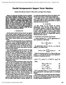
Figure 1. (a) Visualization of an fMRI image from six angles, (b) An illustration of third-order tensor of an fMRI image.

sample X , and then use Xb = JV(1) , · · · , V(M ) K as its KCP −1 factorization, where V(m) = K(m) U(m) for m ∈ [1 : M ]. Upon solution, we can classify the test sample X by using the test kernel matrix.

5. Experiments and Results In order to empirically evaluate the effectiveness of the proposed KSTM, we conduct extensive experiments on reallife neuroimaging (fMRI) data for disease prediction and compare with several state-of-the-art methods. In the following, we introduce the datasets and baselines used and describe how we performed the experiments. Then we present the experimental results as well as the analysis. 5.1. Data Collection and Preprocessing In the experiments, we consider three resting-state fMRI datasets as follows: Alzheimer’s Disease (ADNI): This dataset is collected from the Alzheimer’s Disease Neuroimaging Initiative1 . It contains the resting-state fMRI images of 33 subjects, including patients with Mild Cognitive Impairment (MCI) or Alzheimer’s Disease (AD), and normal controls. We applied SPM8 2 and REST3 to preprocess the data. After this, we averaged each individual image over time domain, resulting in 33 samples of size 61 × 73 × 61. We treat AD+MCI as the negative class, and the normal controls as positive class. Finally, we scaled each individual to [0, 1], as the normalization is very important for group analyses among different subjects. A detailed description of preprocessing is available in (He et al., 2014). Human Immunodeficiency Virus Infection (HIV): This dataset is collected from Chicago Early HIV Infection Study in Northwestern University (Wang et al., 2011), 1

http://adni.loni.usc.edu/ http://www.l.ion.ucl.ac.uk/spm/software/spm8/ 3 http://resting-fmri.sourceforge.net 2

Kernelized Support Tensor Machines Table 2. Summary of compared methods. C is trade-off parameter, σ is kernel width parameter, R is the rank of tensor factorization. Methods Type of Input Data Correlation Exploited Kernel Explored Nonlinear Factorization Parameters

SVM / SVM+PCA Vectors One-way Supervised —— C, σ

Table 3. Classification accuracy deviation) Methods ADNI SVM 0.49 ± 0.02 SVM+PCA 0.50 ± 0.02 K3rd 0.55 ± 0.01 sKL 0.51 ± 0.03 FK 0.51 ± 0.02 STuM 0.52 ± 0.01 DuSK 0.75 ± 0.02 MMKbest 0.81 ± 0.01 MMKcov 0.69 ± 0.01 3D CNN 0.52 ± 0.03 KSTM 0.84 ± 0.03

K3rd Vectors One-way Unsupervised —— C, σ

sKL Matrices One-way Unsupervised Unexplored C, σ

FK Matrices One-way Unsupervised Unexplored C, σ

comparison (mean ± standard HIV 0.70 ± 0.01 0.73 ± 0.03 0.75 ± 0.02 0.65 ± 0.02 0.70 ± 0.01 0.66 ± 0.01 0.74 ± 0.00 0.79 ± 0.01 0.72 ± 0.02 0.75 ± 0.02 0.82 ± 0.02

ADHD 0.58 ± 0.00 0.63 ± 0.01 0.55 ± 0.00 0.50 ± 0.04 0.50 ± 0.00 0.54 ± 0.03 0.65 ± 0.01 0.70 ± 0.01 0.66 ± 0.02 0.68 ± 0.02 0.74 ± 0.02

which contains 83 fMRI brain images of patients with early HIV infection (negative) and normal controls (positive). We used the same preprocessing steps as in ADNI dataset, resulting in 83 samples of size 61 × 73 × 61. Attention Deficit Hyperactivity Disorder (ADHD): This dataset is collected from ADHD-200 global competition dataset4 , which originally contains 776 subjects, either ADHD patients (negative) or normal controls (positive). Since the dataset is unbalanced, we randomly sampled 100 ADHD patients and 100 normal controls for this study. Finally, we averaged each individual over time domain, resulting in 200 samples of size 58 × 49 × 47. 5.2. Baselines and Metrics To establish a comparative study, we use the following nine state-of-the-art methods as baselines, each representing a different strategy. • SVM: It is SVM with RBF kernel, which is the most widely used vector method for classification. In the following methods, we use it as the classifier, if not stated explicitly. • SVM-PCA: It is a vector-based subspace learning algorithm, which first uses PCA to reduce the input dimension and then feeds into SVM model. This method is commonly used to deal with highdimensional classification, in particular fMRI classification (Song et al., 2011; Xie et al., 2009). • K3rd : It is a vector based tensor kernel method, which 4

http://neurobureau.projects.nitrc.org/ADHD200/

STuM Tensor Multi-way —— Unexplored C, σ, R

DuSK Tensor Multi-way Unsupervised Unexplored C, σ, R

MMK Tensor Multi-way Unsupervised Explored C, σ, R

3D CNN Tensor Multi-way Supervised —— Many*

KSTM Tensor Multi-way Supervised Explored γ, C, σ, R

exploits the input tensor along each mode to capture structural information and has been used to analyze fMRI data together with RBF kernel (Park, 2011). • sKL: It is a matrix unfolding based tensor kernel method that defined based on the symmetric KullbackLeibler divergence, and has been used to reconstruct 3D movement (Zhao et al., 2013b). • FK: It is also a matrix unfolding based tensor kernel method, but defined based on multilinear SVD. The constituent kernels are from the class of RBF kernels (Signoretto et al., 2011). • STuM: It is a support tucker machine approach, where the weight tensor parameter is decomposed using the Tucker factorization (Kotsia & Patras, 2011). • DuSK: It is a tensor kernel method based upon CP factorization, which has been used to analyze fMRI data together with RBF kernel (He et al., 2014). • MMK: It is the most recent tensor kernel method based upon KCP factorization (He et al., 2017), which incorporates the KCP into the DuSK. Since the shared kernel matrices involved in KCP are hard to estimate without a prior knowledge, we consider two schemes: first, we randomly generate them and select the best result of 50 repeated times (denoted as MMKbest ). Second, we perform CP factorization for each data sample and use the covariance matrix of each mode as input (denoted as MMKcov ). • 3D-CNN: It is a 3D convolutional neural network extended from 2D version (Gupta et al., 2013), which uses the convolution kernel. The convolution kernel is the cubic filters learned from data, which has a small receptive field, but extends through the full depth of the input volume. Table 2 summarizes the compared methods. We consider eleven methods in total and evaluate their classification performance. For the evaluation where SVM is needed, we apply LibSVM (Chang & Lin, 2011), a widely used implementation of SVM, with RBF kernel as the classifier. We perform 5-fold cross-validation and use classification accuracy as the evaluation measure. This process was repeated 50 times for all methods and the average classification accuracy of each method is reported as the result. The optimal parameters for all methods are determined by grid search. The optimal trade-off parameter is selected

0.8

0.8

0.6

0.6

0.6

0.4

0.4

0.2

0.2

0

Accuracy

0.8

Accuracy

Accuracy

Kernelized Support Tensor Machines

2

4

6

RANK R

8

(a) ADNI

10

0

0.4

0.2

2

4

6

8

10

0

RANK R

(b) HIV

2

4

6

Rank R

8

10

(c) ADHD

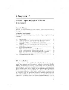
Figure 2. Test accuracy vs. R on (a) ADNI, (b) HIV, and (c) ADHD, where the red triangles indicate the peak positions.

from C ∈ {2−8 , 2−7 , · · · , 28 }, the kernel width parameter is selected from σ ∈ {2−8 , 2−7 , · · · , 28 }, the optimal rank R is selected from {1, 2, · · · , 10}, and the regularized factorization parameter is selected from γ ∈ {2−8 , 2−7 , · · · , 28 }. Note that in the proposed method λ = 1/C. The optimal parameters for 3D-CNN, i.e., receptive field (R), zero-padding (P ), the input volume dimensions (Width × Height × Depth, or W × H × D ) and stride length (S) are tuned based on (Gupta et al., 2013). 5.3. Classification Performance Experimental results in Table 3 shows classification performance of compared methods, where the best result is highlighted in bold type. We can see that the proposed KSTM outperforms all the other methods on three datasets. This is mainly because KSTM can learn the nonlinear relationships embedded within the tensor together with considering prior knowledge across different data samples, while the other methods fail to fully explore the nonlinear relationships or prior knowledge in the tensor object. Specifically, the kernel methods which unfold the input data into vectors or matrices tend to have a lower performance compared to those who preserve the tensor structure. This indicates that unfolding tensor into vectors or matrices would lose the multi-way structural information within tensor, leading to the degraded performance. Besides, KSTM always performs better than DuSK, which empirically shows the effectiveness of feature extraction in tensor data rather than approximation. Compared to MMK method, we can see that a further improvement can be achieved by benefiting from the use of label information during the factorization procedure. These results demonstrate the effectiveness and considerable advantages of the proposed KSTM method for fMRI classification. 5.4. Parameter Sensitivity Although the optimal values of the parameters in our proposed KSTM are found by grid search, it is still important to see the sensitivity of KSTM to the rank of factorization

R. To this end, we vary R ∈ {1, 2, · · · , 10}, while the other parameters are still selected by grid search. Figure 2 shows the variation of test accuracy over different R on three datasets. We can observe that the rank parameter R has a significant effect on the test accuracy and the optimal value of R depends on the data, while in general the optimal value of R lies in the range 2 ≤ R ≤ 6, which may provide a good guidance for selection of the R in advance. In summary, the classification performance of KSTM relies on parameter R, which is difficult to specify the optimal value in advance. However, in most cases the optimal value of R lies in a small range of values and it is not time-consuming to find it using the grid search strategy in practical applications.

6. Conclusion In this paper, we have introduced a Kernelized Support Tensor Machine (KSTM), with an application to neuroimaging classification. Different from conventional kernel methods, KSTM is based on the integration of kernelized tensor factorization with kernel maximum-margin classifier. Typically this is done by defining a joint optimization problem, so that the kernels obtained in KSTM have a greater discriminating power. The kernelized tensor factorization is introduced to capture the complex nonlinear relationships within tensor data, by means of the notion of tensor product RKHS, which supplies a new perspective on tensor factorization methods. Empirical studies on three different neurological disorder prediction tasks demonstrated the superiority of KSTM over existing stateof-the-art tensor classification methods.

Acknowledgements This work is supported in part by NSFC through grants 61503253, 61672357 and 61672313, NSF through grants IIS-1526499 and CNS-1626432, NIH through grant R01MH080636, and the Science Foundation of Shenzhen through grant JCYJ20160422144110140.

Kernelized Support Tensor Machines

References Cao, Bokai, He, Lifang, Kong, Xiangnan, Yu, Philip S., Hao, Zhifeng, and Ragin, Ann B. Tensor-based multiview feature selection with applications to brain diseases. In ICDM, pp. 40–49. IEEE, 2014. Cao, Bokai, He, Lifang, Wei, Xiaokai, Xing, Mengqi, Yu, Philip S., Klumpp, Heide, and Leow, Alex D. t-bne: Tensor-based brain network embedding. In SDM, 2017. Chang, Chih-Chung and Lin, Chih-Jen. Libsvm: a library for support vector machines. ACM Transactions on Intelligent Systems and Technology, 2(3):27, 2011. Chapelle, Olivier. Training a support vector machine in the primal. Neural computation, 19(5):1155–1178, 2007. Cichocki, Andrzej, Mandic, Danilo, De Lathauwer, Lieven, Zhou, Guoxu, Zhao, Qibin, Caiafa, Cesar, and Phan, Huy Anh. Tensor decompositions for signal processing applications: From two-way to multiway component analysis. IEEE Signal Processing Magazine, 32(2):145– 163, 2015.

Liu, Xiaolan, Guo, Tengjiao, He, Lifang, and Yang, Xiaowei. A low-rank approximation-based transductive support tensor machine for semisupervised classification. IEEE Transactions on Image Processing, 24(6): 1825–1838, 2015. Lu, Chun-Ta, He, Lifang, Shao, Weixiang, Cao, Bokai, and Yu, Philip S. Multilinear factorization machines for multi-task multi-view learning. In WSDM, pp. 701–709. ACM, 2017. Lu, Haiping, Plataniotis, Konstantinos N, and Venetsanopoulos, Anastasios N. Mpca: Multilinear principal component analysis of tensor objects. IEEE Transactions on Neural Networks, 19(1):18–39, 2008. Luo, Dijun, Nie, Feiping, Huang, Heng, and Ding, Chris H. Cauchy graph embedding. In ICML, pp. 553–560, 2011. Ma, Guixiang, He, Lifang, Lu, Chun-Ta, Yu, Philip S., Shen, Linlin, and Ragin, Ann B. Spatio-temporal tensor analysis for whole-brain fmri classification. In SDM, pp. 819–827. SIAM, 2016.

Guo, Tengjiao, Han, Le, He, Lifang, and Yang, Xiaowei. A ga-based feature selection and parameter optimization for linear support higher-order tensor machine. Neurocomputing, 144:408–416, 2014.

Park, Sung Won. Multifactor analysis for fmri brain image classification by subject and motor task. Electrical and computer engineering technical report, Carnegie Mellon University, 2011.

Gupta, Ashish, Ayhan, Murat, and Maida, Anthony. Natural image bases to represent neuroimaging data. In ICML, pp. 987–994, 2013.

Rubinov, Mikail, Knock, Stuart A, Stam, Cornelis J, Micheloyannis, Sifis, Harris, Anthony WF, Williams, Leanne M, and Breakspear, Michael. Small-world properties of nonlinear brain activity in schizophrenia. Human brain mapping, 30(2):403–416, 2009.

Hao, Zhifeng, He, Lifang, Chen, Bingqian, and Yang, Xiaowei. A linear support higher-order tensor machine for classification. IEEE Transactions on Image Processing, 22(7):2911–2920, 2013. He, Lifang, Kong, Xiangnan, Yu, Philip S, Yang, Xiaowei, Ragin, Ann B, and Hao, Zhifeng. Dusk: A dual structure-preserving kernel for supervised tensor learning with applications to neuroimages. In SDM, pp. 127– 135, 2014. He, Lifang, Lu, Chun-Ta, Ding, Hao, Wang, Shen, Shen, Linlin, Yu, Philip S., and Ragin, Ann B. Multi-way multi-level kernel modeling for neuroimaging classification. In CVPR, 2017. Kolda, Tamara G and Bader, Brett W. Tensor decompositions and applications. SIAM review, 51(3):455–500, 2009. Kotsia, Irene and Patras, Ioannis. Support tucker machines. In CVPR, pp. 633–640. IEEE, 2011. Kotsia, Irene, Guo, Weiwei, and Patras, Ioannis. Higher rank support tensor machines for visual recognition. Pattern Recognition, 45(12):4192–4203, 2012.

Shao, Weixiang, He, Lifang, and Yu, Philip S. Clustering on multi-source incomplete data via tensor modeling and factorization. In PAKDD, pp. 485–497. Springer, 2015. Signoretto, Marco, De Lathauwer, Lieven, and Suykens, Johan AK. A kernel-based framework to tensorial data analysis. Neural networks, 24(8):861–874, 2011. Signoretto, Marco, Olivetti, Emanuele, De Lathauwer, Lieven, and Suykens, Johan AK. Classification of multichannel signals with cumulant-based kernels. IEEE Transactions on Signal Processing, 60(5):2304–2314, 2012. Signoretto, Marco, De Lathauwer, Lieven, and Suykens, Johan AK. Learning tensors in reproducing kernel hilbert spaces with multilinear spectral penalties. arXiv preprint arXiv:1310.4977, 2013. Song, Sutao, Zhan, Zhichao, Long, Zhiying, Zhang, Jiacai, and Yao, Li. Comparative study of svm methods combined with voxel selection for object category classification on fmri data. PloS one, 6(2):e17191, 2011.

Kernelized Support Tensor Machines

Tao, Dacheng, Li, Xuelong, Wu, Xindong, Hu, Weiming, and Maybank, Stephen J. Supervised tensor learning. Knowledge and Information Systems, 13(1):1–42, 2007. Vapnik, Vladimir. The nature of statistical learning theory. Springer science & business media, 2013. Wang, Senzhang, He, Lifang, Stenneth, Leon, Yu, Philip S., and Li, Zhoujun. Citywide traffic congestion estimation with social media. In GIS, pp. 34. ACM, 2015.

Yan, Shuicheng, Xu, Dong, Yang, Qiang, Zhang, Lei, Tang, Xiaoou, and Zhang, Hong-Jiang. Multilinear discriminant analysis for face recognition. IEEE Transactions on Image Processing, 16(1):212–220, 2007. Zhao, Qibin, Zhou, Guoxu, Adalı, T¨ulay, Zhang, Liqing, and Cichocki, Andrzej. Kernel-based tensor partial least squares for reconstruction of limb movements. In ICASSP, pp. 3577–3581. IEEE, 2013a.

Wang, Xue, Foryt, Paul, Ochs, Renee, Chung, Jae-Hoon, Wu, Ying, Parrish, Todd, and Ragin, Ann B. Abnormalities in resting-state functional connectivity in early human immunodeficiency virus infection. Brain connectivity, 1(3):207–217, 2011.

Zhao, Qibin, Zhou, Guoxu, Adali, Tulay, Zhang, Liqing, and Cichocki, Andrzej. Kernelization of tensor-based models for multiway data analysis: Processing of multidimensional structured data. IEEE Signal Processing Magazine, 30(4):137–148, 2013b.

Xie, Song-yun, Guo, Rong, Li, Ning-fei, Wang, Ge, and Zhao, Hai-tao. Brain fmri processing and classification based on combination of pca and svm. In IJCNN, pp. 3384–3389. IEEE, 2009.

Zhou, Hua, Li, Lexin, and Zhu, Hongtu. Tensor regression with applications in neuroimaging data analysis. Journal of the American Statistical Association, 108(502):540– 552, 2013.