Deep Learning and Support Vector Machine for Effective Plant Identification Gjorgji Strezoski, Dario Stojanovski, Ivica Dimitrovski, and Gjorgji Madjarov Faculty of Computer Science and Engineering, Skopje, 1000, Macedonia,
[email protected],
[email protected],
[email protected],
[email protected] http://www.finki.ukim.mk
Abstract. Our planet is blooming with vegetation that consists of hundreds of thousands of plant species. Each and every one species is unique in its own way, thus enabling people to distinguish one plant from another. Distinguishing plant species is a non trivial task, in fact, it is challenging even for renowned botanists with lots of years of experience in the field. Having in mind the complexity of the task, in this paper we present a system for plant species identification based on Convolutional Neural Networks (CNN’s) and Support Vector Machines (SVM’s). The combination of these two approaches for both feature generation and classification results in a powerful plant identification system. Additionally we report state of the art results using this approach, as well as comparison with other types of approaches on the same dataset. Keywords: deep learning, SVM, support vector machines, plant images, plantCLEF, CNN
1
Introduction
One of the greatest treasures our planet has to offer is a great diversity of plant species scattered around the world. Ranging from small micro vegetation growing in rock cracks to the mighty Adansonia1 (Baobab) tree with a lifespan up to 1275 years, these same plants have played a life sustaining role in the lives of small bug colonies, various mammal groups and even whole ecosystems. Botanical and agricultural scientific improvements have changed the world drastically many times over. Today we rely heavily on botanics and agriculture. Modern architecture, construction, medicine and pharmaceuticals, cosmetic products and even transportation would be unimaginable without the benefits we enjoy from our rich flora. Though seemingly separate and indestructible, there exists a delicate link between the flora and the fauna, which if shattered would have grave consequences on all life on earth. That is why we have to handle them with great caution and adequate knowledge. 1
BaoBab:http://www.plantzafrica.com/plantab/adansondigit.htm
2
If we want to make efficient and smart use of this precious, limited resource without disturbing the fragile nature of our ecosystem, an accurate understanding and knowledge of identity, geographic distribution and uses of plants is essential in the process. Acquiring this knowledge and gaining the understanding necessary for efficient resource harvesting is often pretty difficult. This is due to data incompleteness in high diversity ecosystems or general lack of distribution mediums in less developed areas. This taxonomic glitch in the system is a serious problem for scientists, researchers and professionals alike. As a viable solution of the taxonomic gap issue, image retrieval technologies are considered a cornerstone in the solution of the problem with promising results. Because this presents a very challenging task, the CLEF Cross Language Evaluation forum has been organizing yearly competitions[9] on plant image identification in order to perform a general evaluation of recent advances in the computer vision and information retrieval. Since 2011 there have been tremendous advances in both the competing teams approaches and the dataset available for training and testing. The 2014 competition introduces a new challenge, that is plant observations. This means that there are several observations of one plant regarding different organs or even conditions under which the image is taken. Based on the same image retrieval cornerstone, the system we describe in this paper uses innovative techniques for image retrieval combined with classical machine learning paradigms. Plant image classification is a generally complicated type of classification, because all of the images are both semantically and visually very similar. [6] For example both the leaves of a Japanese maple and a Cleome plant are green, which proves the visual similarity, and both of them are leaves which makes the two items semantically identical. Although upon close examination the texture of both leaves is different and a properly constructed feature would amplify that difference. This leaves no margin for assumptions when it comes to feature generation and even classification. Our system tackles this fine-grained classification problem using a Convolutional Neural Network implementation from Overfeat NYU 2 for image feature extraction and a linear support vector machine from LibSVM 3 . As training and testing data we used the dataset from the CLEF Plant Identification challenge, namely the Pl@ntview dataset. This dataset provided us with 47815 train images and 8163 test images[9]. The rest of this paper is organized as follows: Section 2 gives a brief overview of related projects and work done in this field, while Section 3 provides a detailed specification of our architecture as well as the implementation details starting from pre-training image manipulation to the final prediction phase. Section 4 describes the experimental process with the experimental setup. Section 5 presents the results according to the CLEF metrics and discusses the various circumstances in which the results were calculated. Finally Section 6 concludes this paper. 2 3
OverFeat: http://cilvr.nyu.edu/doku.php?id=code:start LibSVM: http://www.csie.ntu.edu.tw/ cjlin/libsvm/
3
2
Related work
Because of the nature of this work and the data and evaluation measures used by this system it is important to mention the systems of some of the competing teams that participated in the PlantCLEF 2014 Challenge4 . IBM Research, Australia. The winning team of the PlantCLEF 2014 challenge used multiple techniques one of which used a deep Convolutional Neural Network for both feature generation, feature construction and final classification. Their network had 5 Convolutional layers mixed with max pooling layers in the middle. Acting like a classifier, the final section of their network is consisted of three fully connected layers combined with a soft-max layer for classification.[4] At this moment it is important to notice that the Convolutional neural network was pre-trained on the ImageNet5 dataset. Also given the circumstances their fully connected segment was limited to 2048 nodes, as that is enough to validly represent plant images. IBM Research Australia had also submitted a dense SIFT and Fisher vector encoding run which had the best results and won the competition [9]. QUT, Australia. Although not the best team in the competition, they presented an intriguing combination of an extremely Randomized Tree Classifier with a Convolutional Neural Network. In order to speed up the process they changed the output layers of the neural network thus gaining different features with different complexity. After they established the desired complexity, a extremely Randomized Trees Classifier [2] is used in order to output a probability distribution over the 500 species [10], one for each feature. The probability distributions are then averaged in order to compute a single probability distribution for a test image. Finally, probability distributions from several pictures from a same test observation are added in order to obtain the final list of ranked species[9]. PlantNet, France. These participants used for all categories a large scale matching approach, and some shape descriptors in the specific case of LeafScan (Directional Fragment Histogram and standard shape parameters). They extracted numerous local features: SURF, Fourier2D, rotation invariant Local Binary Patterns, Edge Orientation Histogram, weighted RGB, weighted-LUV and HSV histograms. [7] After preliminary evaluations, each type of view had its own subsets of types of local features. These local features are hashed, indexed and searched in separate index with the Random Maximum Margin Hashing approach (one for each type of view and for each type of feature). Then, a hierarchical late fusion scheme is applied in order to combine the image response lists of the different modalities: first from the different types of local [?], then from 4 5
PlantCLEF: http://www.imageclef.org/2014/lifeclef/plant ImageNet: http://www.image-net.org/
4
the multiple-images from a same category, and finally from all the categories in order to obtain a final list related to one plant observation[9].
3
System implementation
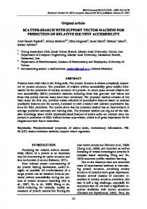
As mentioned earlier, we developed a system for plant identification that is based on Convolutional Neural Networks and Support Vector Machines. We choose a deep architecture for feature extraction over the conventional descriptor and detector combo because of the robustness and complexity of the features extracted with the CNN. Additionally, CNNs also provide the possibility to shorten on prolong the feature extraction time, depending on the time frame available, feature precision and complexity. This is due to the sole nature of neural networks themselves, where every layer can be a potential output. Also there exists a hierarchical feature structure, so as we climb higher up the layers of the CNN we get more detailed and complex features. Another advantage is that the feature dimension is unified throughout the dataset, which implies that there is no need for further feature modification. As soon as the features are generated, they are ready for the classifier. This type of flexibility is very important with tasks like this, having in mind the limited training time and tight deadlines.
Fig. 1. System Architecture
5
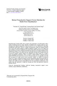
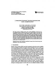
Before any feature extraction takes place we resize and crop the images according to the plant organ. This is done due to simplifying the final feature vectors and faster svm training and predictions. Even though the CNN itself can be used as a classifier, it is possible to append any type of classifier at the chosen output layer of the CNN.[1] We have chosen the SVM approach, as it has been tested multiple times throughout the years and yields high ranking results with features like ours. Additionally, studying the approaches of other teams in plant identification challenges, we have come to the conclusion that SVM approaches report better results in most of the cases. PlantCLEF also presents the challenge of multi-query classification. Every plant that is present in the dataset is photographed from multiple observation points. One observation of one individual-plant is observed the same day by a same author involving several pictures with the same Observation ID. So each observation has its own ID and corresponds to a particular plant. One plant can have up to 8 observations.
S T E M
E NT I R E
F L O WE R
F L O WE R
L E A F
L E A FS C A N
F R U I T
B R A NC H
P L U MT R E E
Fig. 2. Observation and image correlation example
3.1
Dataset modification
Sometimes the background of the images can be noisy and distracting when it comes to classification. That is why it is better to improve the ratio between the subject of the image and the unnecessary background data. Improving this ratio can be done with segmentation - separating the image subject from the rest of the image or just simple cropping, so that we can reduce the amount of background data. In our case some of the images like those in the Fruit, Flower and Leaf categories showed better results when they were cropped by 50px on each side. Cropping requires a trivial check for image dimensions before the operation itself, because an image cannot be cropped to dimensions smaller
6
than 0px. For this purpose we used the crop command from the Pillow library for Python 2.7.4 with the respectful checks and precautions. Figure 2 presents a graphical depiction of the image altering process that takes place before feature extraction.
i )
i i )
Fig. 3. i) This a raw image from the Pl@ntview dataset ii) This is the cropped and reduced final image
The images in the Pl@ntView dataset have variable width and height. When using a Convolutional Neural Network for feature extraction, due to the sliding window approach, the features extracted would have different dimensions depending on the image in question. This type of variability can cause serious implementation problems further on. With this in mind we deliberately reduced the image dimensions to strictly 231px width and 231px height. Which is the dimension of the sliding filter we use for feature extraction. In this case a simple image transformation saves a lot of development and training time in the future because this way we only get a single vector per image. Reducing the dimensions of the images is done without preservation of the image aspect ratio. The robust features of the CNN implementation allows for such irregularities when it comes to feature extraction of distorted images. We performed the dimension adjustment using the latest stable version ImageMagick for Debian OS. 3.2
Feature extraction
Deep architectures have revolutionized the computer vision world [8]. Offering robust and precise features, easy setup and an unprecedented potential for parallelism over GPU, deep architectures have improved results in classification and retrieval challenges multiple times. One of the most frequently used implementation of these deep architecture is the Convolutional Neural Network. We as well have chosen this type of architecture for the feature generation part of our
7
system. Concretely we are using a pretrained network package from OverFeat. This network is pretrained on the ImageNet dataset and offers an easy to use interface for data extraction. Overfeat also offers two types of neural networks for feature extraction or classification. A smaller network that is faster but a little less accurate and a larger, deeper network that improves accuracy but also increases the execution times. For our system we used the smaller Overfeat network. This network outputs a 3 dimensional tensor so that the first dimension correspond to the features, while dimensions two and three are spatial (y and x respectively). One 231x231px patch produces 4096 features which means that if the image is not cropped to exactly 231x231px there will be multiple vectors for the differently cropped regions. Having in mind that this PlantCLEF is a multi-query challenge this would immensely complicate further development. Just assembling and combining the features for multiple observation would prolong the SVM training and prediction times by a couple of times . In our case we use the 19-th layer of the network because it offers the best trade-off between speed and acuracy. 3.3
SVM training and prediction
The latest stable version of LibSVM powers our SVMs [3]. Using the features generated from the CNN we performed training of our classifiers. Having better accuracy in mind we trained one classifier per class in such a way that the images that belong to the class for which the classifier is trained on, were marked as positive and rest as negative. Although it improves accuracy, this resulted in a great imbalance between the number of positive and negative sample in the training process. We solve this problem by adding weights to the classes depending on the number of images that they have. More precisely, the weight assigned to the positive class is calculated in mN eg ; whereas the weight of the negative class the following manner: N mPNos+N mP os N mP os+N mN eg in this manner: . In the formulas NmPos and NmNeg represent N mN eg the number of positive and negative images in the training set, accordingly.[6] Classification was performed using the model created from the generated visual features. Our SVMs use a precomputed χ2y kernel for every class. For score improvement we optimize a cost parameter named C according to the evaluation scores. 3.4
Probability fusion and classification
Having in mind that the images in the test dataset are associated with plant observations to perform multiple image queries for all image organs and scans having the same ObservationID value. The procedure of fusing the information is carried out in 4 steps. We first grouped all the images I2 , ..., Ik coming from the same plant observation using the ObservationID in meta-data.Then, we computed similarity ranking lists of the retrieved images L1 , ..., Lk corresponding
8
to the query images I1 , ..., Ik .Finally, the 300 first image results were kept for each list and were merged into a final list L using a late fusion scheme.[6] We used a probability fusion scheme, first the classes associated to the images from the lists L1 , ..., Lk are ranked per organ (i.e. scans), according to the average L2 distance between the corresponding query images and the images from their ranked lists L1 , ..., Lk . We took into account only the best two ranked images of one observation. The final predictions (per observation) are obtained by calculating the minimal ranks of the classes.[6]
4
Experiments
4.1
Dataset
PlantCLEF is based on the Pl@ntView dataset which focuses on 500 herb, tree and fern species centered on France (some plants observations are from neighboring countries). The training data results in 47815 images (1987 of ”Branch”, 6356 photographs of ”Entire”, 13164 of Flower”, 3753 ”Fruit”, 7754 of ”Leaf”, 3466 ”Stem” and 11335 scans and scan-like pictures of leaf) with complete xml files associated to them. On the other side, the test data results in 8163 plantobservation-queries. These queries are based on 13146 images (731 of ”Branch”, 2983 photographs of ”Entire”, 4559 of Flower”, 1184 ”Fruit”, 2058 of ”Leaf”, 935 ”Stem” and 696 scans and scan-like pictures of leaf). 4.2
Experimental setup
For our experiments we used a HP Z800 Workstation with a 4 Core Intel Xeon processor E5620 that runs on 2.40 GHz with 12MB cache. Our workstation is also equipped with 24 GigaBytes, 1066 MHz RAM memory and a hard disk drive of 1 TB. All of the experiments were run on a 64 bit Debian 3.16.3-2 operating system [5], codename Jessie, running Python 2.7.4 with the latest stable versions of OpenBLAS6 , Mono7 , Pillow 8 and ImageMagick. The computationally demanding functions were optimized on the lowest possible level using advanced parallel features of the latest .Net packages. As mentioned above in the text, feature extraction was performed using the OverFeat Convolutional Neural Network.
5
Results and discussion
The primary metric used to evaluate the submitted runs is a score related to the rank of the correct species in the list of retrieved species. Each plant observation test is attributed with a score between 0 and 1: of 1 if the 1st returned species is correct and will decrease quickly while the rank of the correct species increases. An average score will then be computed on all test individual plants as well.[9] 6 7 8
OpenBLAS: http://www.openblas.net/ Mono: http://www.mono-project.com/ Pillow: https://pypi.python.org/pypi/Pillow/
9
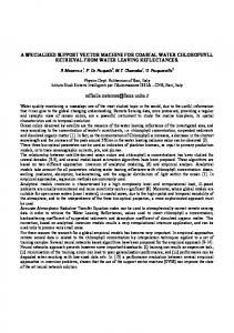
Competing team name Competing team score IBM Australia 0.471 0.325 CURRENT PlantNet 0.289 0.255 BME TMIT QUT 0.249 FINKI 0.205 Sabanci 0.127 I3S 0.091 0.088 SZTE Miracl 0.063 0.043 IV Processing Table 1 presents the overall scores for the complete task of 2014. It is clearly visible that our approach generates promising results. There are many pros to our solution because it scales well and it does not need retraining for different datasets. Robust features and incremental training assure a context independent architecture, which is also proven by the fact that the CNN is trained on a completely different type of dataset. We believe that by improving the training conditions of the CNN and carefully adjusting the train dataset we can gain even better results.
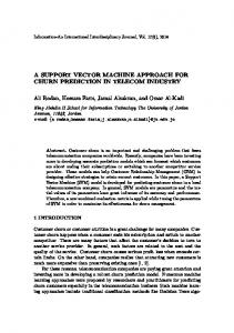
Fig. 4. Evaluation results by organ
Figure 4 demonstrates the PlantCLEF 2014 scores separated by plant organs.
10
6
Conclusion and future work
In the end, after the completion of all the experiments and the experience we had through the whole process, we have only excellent remarks regarding deep architectures when it comes to image classification and retrieval. In future we will explore the possibility of training a CNN on only plant data and try to generate even better feature filters with hopes of improved results and faster training and prediction times.
7
Acknowledgments
We would like to acknowledge the support of the European Commission through the project MAESTRA - Learning from Massive, Incompletely annotated, and Structured Data (Grant number ICT-2013-612944).
References R in Ma1. Bengio, Y.: Learning deep architectures for ai. Foundations and trends chine Learning 2(1), 1–127 (2009) 2. Bosch, A., Zisserman, A., Muoz, X.: Image classification using random forests and ferns. In: Computer Vision, 2007. ICCV 2007. IEEE 11th International Conference on. pp. 1–8. IEEE (2007) 3. Chang, C.C.: Libsvm: Introduction and benchmarks. http://www. csie. ntn. edu. tw/˜ cjlin/libsvm (2000) 4. Chen, Q., Abedini, M., Garnavi, R., Liang, X.: Ibm research australia at lifeclef2014: Plant identification task. In: Working notes of CLEF 2014 conference (2014) 5. Debian, G.: Linux (2005) 6. Dimitrovski, I., Madjarov, G., Lameski, P., Kocev, D.: Maestra at lifeclef 2014 plant task: Plant identification using visual data. In: Working notes of CLEF 2014 conference (2014) 7. Go¨eau, H., Joly, A., Yahiaoui, I., Bakic, V., Verroust-Blondet, A., Bonnet, P., Barth´el´emy, D., Boujemaa, N., Molino, J.F.: Plantnet participation at lifeclef2014 plant identification task. In: CLEF2014 Working Notes. Working Notes for CLEF 2014 Conference, Sheffield, UK, September 15-18, 2014. pp. 724–737. CEUR-WS (2014) 8. Hinton, G., Osindero, S., Teh, Y.W.: A fast learning algorithm for deep belief nets. Neural computation 18(7), 1527–1554 (2006) 9. Joly, A., Go¨eau, H., Glotin, H., Spampinato, C., Bonnet, P., Vellinga, W.P., Planque, R., Rauber, A., Fisher, R., M¨ uller, H.: Lifeclef 2014: multimedia life species identification challenges. In: Information Access Evaluation. Multilinguality, Multimodality, and Interaction, pp. 229–249. Springer International Publishing (2014) 10. Sz˝ ucs, G., Papp, D., Lovas, D.: Viewpoints combined classification method in image-based plant identification task (2014)
..