Supporting Graph-Based Real-Time Applications in Distributed Systems

Supporting Graph-Based Real-Time Applications in Distributed Systems∗ Cong Liu and James H. Anderson Supporting Soft Real-Time DAG-based Systems on Multiprocessors with No Utilization Loss Department of Computer Science, University of North Carolina at Chapel Hill Abstract

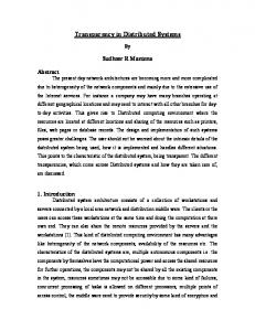
job release AVI Splitter

The processing graph method (PGM) is a widely used framework for modeling applications with producer/consumer precedence constraints. PGM was originally developed by the U.S. Navy to model signal-processing applications where data communications exist among connected tasks. Prior work has shown how to schedule PGMspecified systems on uniprocessors and globally-scheduled multiprocessors. In this paper, this work is extended to enable such systems to be supported in a distributed collection of multicore machines. In such a context, pure global and partitioned scheduling approaches are problematic. Moreover, data communication costs must be considered. In this paper, a clustered scheduling algorithm is proposed for soft real-time PGM-specified distributed task systems for which bounded deadline tardiness is acceptable. This algorithm is effective in reducing data communication costs with little utilization loss. This is shown both analytically and via experiments conducted to compare it with an optimal integer linear programming solution.

1

Video Processing

Audio Processing

FLV Filter

RTSS’10

job deadline

AVI Splitter Video Processing Audio Processing FLV Filter

UNC Chapel Hill

Figure 1:LiuExample DAG. and Anderson

6

of which may be controlled by a multicore machine. The overall collection of such machines is expected to support DAG-based real-time workloads such as radar and signalprocessing subsystems. To support such workloads, efficient scheduling algorithms are needed. Motivated by applications such as this, this paper is directed at supporting real-time DAG-based applications in distributed systems. We view a distributed system as a collection of clusters of processors, where all processors in a cluster are locally connected (i.e., on a multicore machine). A DAG-based task system can be deployed in such a setting by (i) assigning tasks to clusters, and (ii) determining how to schedule the tasks in each cluster. In addressing (i), overheads due to data communications among connected tasks must be considered since tasks within the same DAG may be assigned to different clusters. In addressing (ii), any employed scheduling algorithm should seek to minimize utilization loss. Within a cluster, precedence constraints can easily be supported by viewing all deadlines as hard and executing tasks sporadically (or periodically), with job releases adjusted so that successive tasks execute in sequence. Fig. 1 shows an example multimedia application, which transforms an input AVI video file into a FLV video file (AVI and FLV are two types of multimedia container formats). This application is represented by a DAG with four sporadic tasks. (DAG-based systems are formerly defined in Sec. 2.) Fig. 1 shows a global-earliest-deadline-first (GEDF) schedule for this application on a two-processor cluster. (It suffices to know here that the k th job of the AVI splitter task, the video processing task [or the audio processing task], and the FLV filter task, respectively, must execute in sequence.) As seen in this example, the timing guarantees provided by the sporadic model ensure that any DAG executes correctly as long as no deadlines are missed.

Introduction

In work on real-time scheduling in distributed systems, task models where no inter-task precedence constraints exist, such as the periodic and the sporadic task models, have received much attention. However, in many real-time systems, applications are developed using processing graphs [7, 10], where vertices represent sequential code segments and edges represent precedence constraints. For example, multimedia applications and signal-processing algorithms are often specified using directed acyclic graphs (DAGs) [9, 10]. With the growing prevalence of multicore platforms, it is inevitable that such DAG-based real-time applications will be deployed in distributed systems where multicore machines are used as per-node computers. One emerging example application where such a deployment is expected is fractionated satellite systems [8]. Such a system consists of a number of wirelessly-connected small satellites, each ∗ Work supported by NSF grants CNS 0834270, CNS 0834132, and CNS 1016954; ARO grant W911NF-09-1-0535; AFOSR grant FA9550-09-10549; and AFRL grant FA8750-11-1-0033.

1

Unfortunately, if all deadlines of tasks assigned to the same cluster must be viewed as hard, then significant processing capacity must be sacrificed, due to either inherent schedulability-related utilization loss—which is unavoidable under most scheduling schemes [6]—or high runtime overheads—which typically arise in optimal schemes that avoid schedulability-related loss [4]. In systems where less stringent notions of real-time correctness suffice, such utilization loss can be avoided by viewing deadlines as soft. In this paper, such systems are our focus; the notion of soft real-time correctness we consider is that deadline tardiness is bounded. To the best of our knowledge, in all prior work on supporting DAG-based applications in systems with multiple processors (multiprocessors or distributed systems), either global or partitioned scheduling has been assumed. Under global scheduling, tasks are scheduled from a single run queue and may migrate across processors; in contrast, under partitioned schemes, tasks are statically bound to processors and per-processor schedulers are used. Partitioned approaches are susceptible to bin-packing-related schedulability limitations, which global approaches can avoid. Indeed, if bounded deadline tardiness is the timing constraint of interest, then global approaches can often be applied on multiprocessor platforms with no loss of processing capacity [13]. However, the virtues of global scheduling come at the expense of higher runtime overheads. In work on ordinary sporadic (not DAG-based) task systems, clustered scheduling, which combines the advantages of both global and partitioned scheduling, has been suggested as a compromise [3, 5]. Under clustered scheduling, tasks are first partitioned onto clusters of cores, and intra-cluster scheduling is global. In distributed systems, clustered scheduling algorithms are a natural choice, given the physical layout of such a system. Thus, such algorithms are our focus here. Our specific objective is to develop clustered scheduling techniques and analysis that can be applied to support DAGs, assuming that bounded deadline tardiness is the timing guarantee that must be ensured. Our primary motivation is to develop such techniques for use in distributed systems, where different clusters are physically separated; however, our results are also applicable in settings where clusters are tightly coupled (e.g., each cluster could be a socket in a multi-socket system). Our results can be applied to systems with rather sophisticated precedence constraints. To illustrate this, we consider a particularly expressive DAG-based formalism, the processing graph method (PGM) [12]. PGM was first developed by the U.S. Navy to model signal-processing applications where producer/consumer relationships exist among tasks. In a distributed system, it may be necessary to transfer data from a producer in one cluster to a consumer in another through an inter-cluster network, which could cause a significant amount of data communication overhead. Thus,

any proposed scheduling algorithm should seek to minimize such inter-cluster data communication. Related work. To our knowledge, DAGs have not been considered before in the context of clustered real-time scheduling algorithms, except for the special cases of partitioned and global approaches.1 An overview of work on scheduling DAGs in a distributed system under partitioned approaches (which we omit here due to space constraints) can be found in [14]. The issue of scheduling PGM graphs on a uniprocessor was extensively considered by Goddard in his dissertation [10]. Goddard presented techniques for mapping PGM nodes to tasks in the rate-based-execution (RBE) task model [11], as well as conditions for verifying the schedulability of the resulting task set under a rate-based, earliest-deadline-first (EDF) scheduler. In recent work [14], we extended Goddard’s work and showed that a variety of global scheduling algorithms can ensure bounded deadline tardiness in general DAG-based systems with no utilization loss on multiprocessors, including algorithms that are less costly to implement than optimal algorithms. Contributions. In this paper, we show that sophisticated notions of acyclic precedence constraints can be efficiently supported under clustered scheduling in a distributed system, provided bounded deadline tardiness is acceptable. The types of precedence constraints we consider are those allowed by PGM. We propose a clustered scheduling algorithm called CDAG that first partitions PGM graphs onto clusters, and then uses global scheduling approaches within each cluster. We present analysis that gives conditions under which each task’s maximum tardiness is bounded. Any clustered approach is susceptible to some bin-packing-related utilization loss; however, the conditions derived for CDAG show that for it, such loss is small. To assess the effectiveness of CDAG in reducing inter-cluster data communications, we compare it with an optimal integer linear programming (ILP) solution that minimizes inter-cluster data communications when partitioning PGM graphs onto clusters. We assume that tasks are specified using a rate-based task model that generalizes the periodic and sporadic task models. Organization. The rest of this paper is organized as follows. Sec. 2 describes our system model. In Sec. 3, the ILP formulation of the problem and the polynomial-time CDAG algorithm and its analysis are presented. Sec. 4 evaluates the proposed algorithm via an experimental study. Sec. 5 concludes. 1 The problem of non-real-time DAG scheduling in parallel and distributed systems has been extensively studied. An overview on such work can be found in [15].

2

2

Preliminaries

T1

In this section, we present an overview of PGM and describe the assumed system architecture. For a complete description of the PGM, please see [12].

ρ112=4 T11 θ112=7 σ112=3

2 ρ124=1 T1

T2

ρ113=4 θ113=5 σ113=3 T13

PGM specifications. An acyclic PGM graph system [12] consists of a set of acyclic PGM graphs (DAGs), each with a distinct source node. Each PGM graph contains a number of nodes connected by edges. A node can have outgoing or incoming edges. A source node, however, can only have outgoing edges. Each directed edge in a PGM graph is a typed first-in-first-out queue, and all nodes in a graph are assumed to be reachable from the graph’s source node. A producing node transports a certain number of data units2 to a consuming node, as indicated by the data type of the corresponding queue. Data is appended to the tail of the queue by the producing node and read from the head by the consuming node. A queue is specified by three attributes: a produce amount, a threshold, and a consume amount. The produce amount specifies the number of data units appended to the queue when the producing node completes execution. The threshold amount specifies the minimum number of data units required to be present in the queue in order for the consuming node to process any received data. The consume amount is the number of data units dequeued when processing data. We assume that the queue that stores data is associated with the consuming node. That is, data is stored in memory local to the corresponding consuming node.3 The only restriction on queue attributes is that they must be non-negative integral values and the consume amount must be at most the threshold. In the PGM framework, a node is eligible for execution when the number of data units on each of its input queues is over that queue’s threshold. Overlapping executions of the same node are disallowed. For any queue connecting nodes Tlj and Tlk in a PGM graph Tl , we let ρjk l denote its produce amount, θljk denote its threshold, and σljk denote the consume amount. If there is an edge from task Tlk to task Tlh in graph Tl , then Tlk is called a predecessor task of Tlh . We let pred(Tlh ) denote the set of all predecessor tasks of Tlh . We define the depth of a task within a graph to be the number of edges on the longest path between this task and the source task of the corresponding graph.

ρ212=4 θ212=5

ρ134=2

θ1 θ1 σ124=2 T14 σ134=4 24=3

T21

σ212=3

34=6

T22

(a) Example PGM graph system

T1 (x12=4,y12=12, d12=3,e12=2)

T11

T12

T13

T14

T2

(x11=1,y11=4, d11=4, e11=1)

T21

(x21=1, y21=4, d21=4, e21=2)

T22

(x22=4, y22=12, d22=4, e22=2)

(x13=4,y13=12, d13=3,e13=1)

(x14=2,y14=12, d14=6,e14=2)

(b) Rate-based counterpart of (a) Cluster C1 with 2 processors

Cluster C2 with 2 processors

Interconnection Network B=2

(c) An example distributed system

Figure 2: Example system used throughout the paper. below). Note that, even if all source nodes execute according to a periodic/sporadic pattern, non-source nodes may still execute following a rate-based pattern [10, 14]. The execution rate of a node within a PGM graph can be calculated based upon the attributes of the node’s incoming edges using techniques presented in [10, 14]. According to the rate-based task model [11,14], each task Tlh within a PGM graph Tl is specified by four parameters: (xhl , ylh , dhl , ehl ). The pair (xhl , ylh ) represents the maximum execution rate of Tlh : xhl is the maximum number of invocations of the task in any interval [j ·ylh , (j +1)·ylh ) (j ≥ 0) of length ylh ; such an invocation is called a job of Tlh . xhl and ylh are assumed to be non-negative integers. Additionally, dhl is the task’s relative deadline, and ehl is its worst-case execution time. dhl is defined to be

Example. Fig. 2(a) shows an example PGM graph system consisting of two graphs T1 and T2 where T1 contains four nodes with four edges and T2 contains two nodes with one edge. We will use this example to illustrate other concepts throughout the paper. In the PGM framework, it is often assumed that each source node executes according to a rate-based pattern (see

dhl = ylh /xhl .

(1)

h The j th job of Tlh is denoted Tl,j . We denote its release time h h (when Tl is invoked) as rl,j and its (absolute) deadline as h dhl,j = rl,j + dhl .

(2) xh

The utilization of Tlh , uhl , is defined to be ehl · yhl . The l utilization of a PGM graph T is defined to be ul = l P h u . The widely-studied sporadic task model is a Tlh ∈Tl l special case of the rate-based task model. In the sporadic

2 We

assume that data units are defined so that the number of such units produced reflects the total size of the data produced. 3 It is more reasonable to associate a queue with the corresponding consuming node than with the producer node because this enables the consumer to locally detect when the queue is over threshold and react accordingly.

3

Example. An example distributed system containing two clusters each with two processors interconnected by a network is shown in Fig. 2(c).

T11(1,4, 4,2)

(a) Sporadic releases. T11(1,4, 4,2) 0

4

8

12

(b) Rate-based releases.

16

3

time

In this section, we propose Algorithm CDAG, a clusteredscheduling algorithm that ensures bounded tardiness for DAG-based systems on distributed clusters. Since intercluster data communication can be expensive, CDAG is designed to reduce such communication. CDAG consists of two phases: an assignment phase and an execution phase. The assignment phase executes offline and assigns each PGM graph to one or more clusters. In the execution phase, PGM graphs are first transformed to ordinary sporadic tasks (where no precedence constraints arise), and then scheduled under a proposed clustered scheduling algorithm.

Figure 3: Sporadic and rate-based releases. task model, a task is released no sooner than every p time units, where p is the task’s period. In the rate-based task model, the notion of a “rate” is much more general. Example. Fig. 2(b) shows the rate-based counterpart of the PGM graphs in Fig. 2(a). Fig. 3 shows job release times for task T11 (1, 4, 4, 1) of graph T1 . In inset (a), jobs are released sporadically, once every four time units in this case. Inset (b) shows a possible job-release pattern that is not sporadic. As seen, the second job is released at time 7.5 while the third job is released at time 9.5. The separation time between these jobs is less than that seen in the sporadic schedule. h A job Tl,j may be restricted from beginning execution until certain jobs of tasks in pred(Tlh ) have completed (i.e., h Tl,j cannot start execution until receiving the required data from these jobs). We denote the set of such predecessor h h jobs as pred(Tl,j ). pred(Tl,j ) can be defined precisely by examing the execution rates of all tasks on any path from the source node of Tl to Tlh [14]. We require that for any job h w Tl,j and one of its predecessor jobs, Ti,v , h w rl,j ≥ ri,v

Algorithm CDAG

3.1

Assignment Phase

The assignment phase assigns acyclic PGM graphs (or DAGs for short) to clusters in a way such that the intercluster data communication cost is reduced. Note that the total utilization of the DAGs (or portions of DAGs) assigned to a cluster must not exceed the total capacity of that cluster. CDAG contains an assignment algorithm that is designed to partition DAGs onto clusters such that both the inter-cluster data communication cost and any bin-packing-related utilization loss are minimized. To provide a better understanding of the problem of partitioning DAGs onto clusters with minimum inter-cluster data communication cost, we first formulate it as an ILP, which provides an optimal solution. (Note that, due to potential utilization loss arising from partitioning DAGs, the ILP approach may not find a feasible assignment. However, if the ILP approach cannot find a feasible solution, then the given task set cannot be assigned to clusters under any partitioning algorithm.)

(3)

holds. h If a job Tl,j completes at time t, then its tardiness is defined as max(0, t − dhl,j ) and its response time is defined as h max(0, t − rl,j ). A PGM graph’s tardiness is the maximum of the tardiness of any job of any of its tasks. Note that, when a job of a task misses its deadline, the release time of the next job of that task is not altered. However, jobs of the same task still cannot execute in parallel.

Definition 1. For any edge ejk i of DAG Ti , its edge data xji weight, wijk , is defined to be ρjk i · j . A larger edge data yi weight indicates a larger data communication cost between tasks connected by the corresponding edge. For any edge jk ejk i of DAG Ti , its communication cost $i is defined to jk be wi if the corresponding connected nodes Tij and Tik are assigned to different clusters, and 0 otherwise.

System architecture. We consider the problem of scheduling a set of n acyclic PGM graphs on ϕ clusters C1 , C2 , ..., Cϕ . Each cluster Ci contains λi processors. Clusters are connected by a network. Let B denote the minimum number of data units that can be transferred between any two clusters per time unit. Similarly, let b denote the minimum number of data units that can be transferred between any two processors within the same cluster per time unit. If the system is a distributed collection of multicore machines, then B is impacted by the speed and bandwidth of the communication network and b is impacted by the speed of the data transfer bus on a multicore chip. In this case, b  B, as local on-chip data communication is generally much faster than communication across a network.

Note that the above definition does not consider data consuming rates. This is because data is stored in memory local to the consuming node, as discussed in Sec. 2. Thus, only produced data needs to be transferred. Example. For task T11 of DAG T1 in Fig. 2, we can use previous techniques [10, 14] to calculate its execution rates, 4

ASSIGN

which are x11 = 1 and y11 = 4. Thus, for edge e12 1 of T1 , its 1 1 12 12 x1 edge data weight w1 = ρ1 · y1 = 4 · 4 = 1. Intuitively,

u(Ci ): CAPACITY OF CLUSTER Ci , INITIALLY u(Ci ) = λi ξ: A LIST OF CLUSTERS {C1 , C2 , ..., Cϕ } ζ: A LIST OF DAG S {T1 , T2 , ..., Tn }

1

node T11 produces one data unit on average on edge e12 1 per time unit, given its execution rate (x11 , y11 ) = (1, 4).

P HASE 1: 1 Order DAGs in ζ by largest average data weight first 2 Order clusters in ξ by smallest capacity first 3 for each DAG Ti in ζ in order 4 for each cluster Cj in ξ in order 5 if ui ≤ u(Cj ) 6 Assign all tasks of Ti to Cj 7 Remove Ti from ζ; u(Cj ) := u(Cj ) − ui P HASE 2: 8 for each DAG Ti in ζ in order 9 Order tasks within Ti by smallest depth first, then order tasks within Ti and at the same depth by largest task data weight first 10 Order clusters in ξ by largest capacity first 11 for each task Tik of DAG Ti in ζ in order 12 for each cluster Cj in ξ in order 13 if uki ≤ u(Cj ) then 14 Assign Tik to Cj ; u(Cj ) := u(Cj ) − uki 15 else Remove Cj from ξ

Definition 2. The total communication cost of any given DAG-based system τ , denoted $sum , is given by P P jk Ti ∈τ ejk ∈Ti $i . i

ILP formulation. We are given a set τ of tasks (each task corresponds to a node in a DAG) and a set ξ of clusters. To reduce clutter in the ILP formulation, we denote tasks more simply as T1 , T2 , ..., and let wi,j be the data weight of the edge connecting tasks Ti and Tj (wi,j = 0 if i and j are not connected). (This simplified notation is used only for the ILP formulation.) For all Ti ∈ τ , let xi,k be a binary decision variable that equals 1 when task Ti is assigned to cluster Ck , and 0 otherwise. For all (Ti , Tj ) ∈ τ × τ , let yi,j be a binary decision variable that equals 1 if tasks Ti and Tj are assigned to the same cluster, and 0 otherwise. Our goal is to minimize the total communication cost. An ILP formulation of this optimization problem is then: Minimize P

i∈τ

P

j∈τ

wi,j · (1 − yi,j )

Algorithm ASSIGN algorithm. assigns DAGs Figure 4:description. PsuedocodeAlgorithm of the assignment to clusters in two phases. In the first phase (lines 1-7), it assigns DAGs in largest-average-data-weight-first order to A polynomial-time assignment algorithm. Although the clusters in smallest-capacity-first order, which gives a higher ILP solution is optimal, it has exponential time complexpossibility for DAGs with larger average data weight to be ity. Weassigned now propose a polynomial-time algorithm to assign fully to a cluster. DAGs that cannot be assigned to DAGs to clusters. This algorithm tries to minimize total clusters in the first phase are considered in the secondthe phase communication cost, which is achieved (lines 8-15). For each unassigned DAGbyinlocally order, minimizits tasks ing communication costs when assigning each DAG. are ordered by depth and then tasks at the same depth are ordered by data weight, whichj gives tasks with larger data Definition 3. For any task T of DAG Ti , its task data weight a jhigher possibility toPbei assignedjkto the samejclusterk j weight, w , to be k wi , where Ti → Ti i is defined as their predecessor tasks (linesT8-9). i →TiThen each task in order j denotes that Ttoi clusters has an outgoing edge to Tik . order (lines is assigned in largest-capacity-first k 10-15). Task Ti is assigned to cluster Cj if Tik can receive Definition 4. of Foritsany DAG Tifrom , its average weight, wi , its full share Cj (linesdata 13-14). If not, P utilization jk w jk then Cj is excluded from ibeing considered for any of the e ∈T i islater defined to and be thei next cluster , where Ei will is thebetotal number tasks, in order considered Ei k scheduling of edges in Ti . TA DAG15). Ti ’s data weight is defined to be i (line Pfor jk w . jk Example. ei ∈Ti i Consider the example DAG system in Fig. 2 to be partitioned under the proposed algorithm. 12 By Defs. 1 Example. For an DAG T1 indata Fig.weight 2, by Def. 1, and w1 T= w113an= and 2, T1 has average of 3/4 2 has 1,average w124 = data 1/3,weight and w134 Def. 4,before T1 hasT1an of = 1. 2/3. Thus,Thus, T2 isby ordered . 3 1 average weight of . By Def. 3, task T of T1 hasofa Since Tdata has a utilization of 7/6 and T has a utilization 1 4 2 1 12 data weight of w11of= + w113 = T11 19/12, the tasks T2ware to 2. theIntuitively, first cluster,node and the 1 assigned produces two data units on oncluster, its outgoing tasks of T assigned to average the second whichedges leads per to 1 are time unit, its execution rate (x11 , y11 ) = (1, 4). $sum = given 0. The complexity. proposed DAG algorithm, denoted ASTime Theassignment time complexity of Phase 1 of ASSIGN, is shown in Fig. 4. SIGN depends on (i) the sorting process (lines 1-2), which is

(4)

subject to the constraints below. Note that by Defs. 1 and 2, (4) represents the total communication cost. • Each task must be assigned to one cluster: P

Ck ∈ξ

xi,k = 1, ∀Ti ∈ τ.

• The total utilization of all tasks assigned to a cluster must not exceed the total capacity of that cluster: P

Ti ∈τ

xi,k · ui ≤ λk , ∀Ck ∈ ξ.

• yi,j should be 1 when two tasks are assigned to the same cluster, and 0 otherwise: yi,j ≤ xi,k − xj,k + 1, ∀(Ti , Tj ) ∈ τ × τ, ∀Ck ∈ ξ, yi,j ≤ −xi,k + xj,k + 1, ∀(Ti , Tj ) ∈ τ × τ, ∀Ck ∈ ξ. By solving the ILP above, we obtain an optimal assignment that gives the minimum total communication cost as long as there exists a feasible assignment. Example. Consider assigning DAGs T1 and T2 in Fig. 2 to two clusters. T1 has a utilization of 1/4+2/3+1/3+1/3 = 19/12 and T2 has a utilization of 1/2 + 2/3 = 7/6. By formulating this assignment problem as an ILP according to the above approach, an optimal solution is to assign all tasks of T1 to the first cluster and all tasks of T2 to the second cluster, which leads to $sum = 0.

Algorithm description. Algorithm ASSIGN assigns DAGs to clusters in two phases. In the first phase (lines 1-7), it 6 assigns DAGs in largest-average-data-weight-first order to 5

O(n · logn) 3-4), which of O(n · log complexity process (lin where µ is (ii) the two where N is corresponds complexity Since N > O(n · logn)

Partitionin condition f DAG-based us denote ta after orderin that are ful sumed to b denote the u stating the t Lemma 1. first Pi task t k=1 u(Tk largest task

Proof. Due to any clus executed. I to assign th ter Cϕ does Moreover, f there exists Cj , and thu commodate again for an such cluste the utilizati Ti ). Thus, f greater than have been s tasks is eq which is giv

⇔

Pi

P

k=

⇔ ⇒

{beca

clusters in smallest-capacity-first order, which gives a higher possibility for DAGs with larger average data weight to be fully assigned to a cluster. DAGs that cannot be assigned to clusters in the first phase are considered in the second phase (lines 8-15). For each unassigned DAG in order, its tasks are ordered by depth and then tasks at the same depth are ordered by data weight, which gives tasks with larger data weight a greater chance to be assigned to the same cluster as their predecessor tasks (lines 8-9). Then each task in order is assigned to clusters in largest-capacity-first order (lines 10-15). Task Tik is assigned to cluster Cj if Tik can receive its full share of its utilization from Cj (lines 13-14). If not, then Cj is excluded from being considered for any of the later tasks, and the next cluster in order will be considered for scheduling Tik (line 15).

to assign the ith task Ti to any cluster, then the last cluster Cϕ does not have enough capacity to accommodate Ti . Moreover, for each previous cluster Cj , where j ≤ ϕ − 1, there exists a task, denoted T j , that could not be assigned to Cj , and thus the next cluster in order was considered to accommodate T j and Cj was removed from being considered again for any of the later tasks (line 15). That is, for each such cluster Cj , its remaining capacity is strictly less than the utilization of T j (for the last cluster, we know that T ϕ is Ti ). Thus, for any cluster Cj , its allocated capacity is strictly greater than λj − u(T j ). Since tasks {T1 , T2 , ..., Ti−1 } have been successfully assigned, the total utilization of these tasks is equal to P the total allocated capacity of clusters, i−1 which is given by k=1 u(Tk ). Hence, we have

Example. Consider the example DAG system in Fig. 2 to be partitioned under the proposed algorithm. By Defs. 1 and 2, T1 has an average data weight of 3/4 and T2 has an average data weight of 1. Thus, T2 is ordered before T1 . Since T2 has a utilization of 7/6 and T1 has a utilization of 19/12, the tasks of T2 are assigned to the first cluster, and the tasks of T1 are assigned to the second cluster, which leads to $sum = 0.

Pi−1

Pϕ u(Tk ) > j=1 (λj − u(T j )) {adding u(Ti ) on both sides} Pi Pϕ j k) > k=1 u(TP j=1 (λj − u(T )) + u(Ti ) ϕ {because j=1 λj = m and u(T ϕ ) = u(Ti )} Pi Pϕ−1 j k=1 u(Tk ) > m − j=1 u(T ) {by the definition of uϕ−1 } Pi k=1 u(Tk ) > m − uϕ−1 . k=1

⇔ ⇔ ⇒

Theorem 1. Algorithm ASSIGN successfully partitions any DAG-based task system τ on ϕ clusters for which usum ≤ m − uϕ−1 .

Time complexity. The time complexity of Phase 1 of ASSIGN depends on (i) the sorting process (lines 1-2), which is O(n · logn + ϕ · logϕ), and (ii) the two for loops (lines 3-4), which is O(N · ϕ), where N is the number of tasks in the system (each task corresponds to a node in a DAG). Thus, Phase 1 has a time complexity of O(n · logn + ϕ · logϕ + N · ϕ). The time complexity of Phase 2 of ASSIGN depends on (i) the sorting process (lines 9-10), which is O(n·µ·logµ+ϕ·logϕ), where µ is the maximum number of tasks per-DAG, and (ii) the two for loops (lines 11-12), which is O(N · ϕ). Thus, Phase 2 has a time complexity of O(n·µ·logµ+ϕ·logϕ+N ·ϕ). The overall time complexity of ASSIGN is thus O(n·logn+ϕ·logϕ+n·µ·logµ+N ·ϕ).

Proof. Let us suppose that Algorithm ASSIGN fails to asth sign Pi the i task Ti to any cluster. Then by Lemma 1, k=1 u(Tk ) > m − uϕ−1 holds. Therefore, we have ⇒

PN

Pi

k=1

k=1

u(Tk ) > m − uϕ−1

u(Tk ) = usum > m − uϕ−1 .

Hence, any system that Algorithm ASSIGN fails to partition must have usum > m − uϕ−1 . If ϕ is much smaller than m, which will often be the case in practice, then the proposed assignment algorithm results in little utilization loss even in the worst case.

Partitioning condition. The following theorem gives a condition for ASSIGN to successfully partition any given DAG-based task system onto clusters. For conciseness, let us denote tasks (each task corresponds to a node in a DAG) after ordering by T1 , T2 , ..., TN (note that tasks within DAGs that are fully assigned to clusters in the first phase are assumed to be ordered before all other tasks here). Let u(Ti ) denote the utilization of task Ti under this notation. Before stating the theorem, we first prove the following lemma.

Bounding $sum . For any given DAG system, if all DAGs can be assigned in the first phase, then $sum = 0. In the second phase, each DAG is considered in order, and if a cluster fails to accommodate a task (line 15), then it will never be considered for later tasks. Thus, it immediately follows that at most ϕ − 1 DAGs can contribute to $sum . Due to the fact that in the worst case all edges of a DAG can cause inter-cluster communication (as illustrated by the example below), an upper-bound on $sum under Algorithm ASSIGN is given by the sum of ϕ − 1 largest DAG data weights.

Lemma 1. Under Algorithm ASSIGN, if a task Ti is the first Pi task that cannot be assigned to any cluster, then k=1 u(Tk ) > m − uϕ−1 , where uϕ−1 is the sum of ϕ − 1 largest task utilizations.

Example. Consider a scenario where three DAGs Ti , Tj , and Tk are assigned to three clusters in a way as shown in Fig. 5. Note that all edges of ϕ − 1 = 2 DAGs Tj and Tk contribute to $sum .

Proof. Due to the fact that some task Ti cannot be assigned to any cluster, the second phase of Algorithm ASSIGN is executed. In the second phase, if Algorithm ASSIGN fails 6

2

RTSS’10

Supporting Soft Real-Time DAG-based Systems on Multiprocessors with No Utilization Loss

Assigned to the first cluster

Tj 1

Ti 1

Ti 2

Ti 3

Tj 2

Tj 3

h release time, denoted r(Tl,j ), is given by

Assigned to the second cluster

h r(Tl,j )

T k1

Tj 4

T k2

T k3

T k4

Assigned to the third cluster

Figure 5: Example worst-case scenario where all edges of and7Anderson ϕ − 1 DAGs contribute toLiuthe total communication cost.

UNC Chapel Hill

3.2

69

Scheduling Phase

h h = max rl,j , r(Tl,j−1 ) + dhl ,
h h Fmax (pred(Tl,j ), υl,j ) .

Given that a source task has no predecessors, the rede1 1 fined release of any job Tl,j (j > 1) of such a task, r(Tl,j ), is given by
1 1 1 r(Tl,j ) = max rl,j , r(Tl,j−1 ) + d1l . (6) h For the first job Tl,1 (h > 1) of any non-source task, its h redefined release, r(Tl,1 ), is given by


h h h h r(Tl,1 ) = max rl,1 , Fmax (pred(Tl,j ), υl,j ) .

After executing the assignment phase, every task is mapped to a cluster. The scheduling phase of CDAG ensures that each task is scheduled with bounded tardiness. The scheduling phase consists of two steps: (i) transform each PGM graph into ordinary sporadic tasks by redefining job releases, and (ii) apply any window-constrained scheduling policy [13] such as GEDF to globally schedule the transformed tasks within each cluster.

(5)

(7)

1 Finally, for the first job Tl,1 of any source task, its release time is not altered, i.e., 1 1 r(Tl,1 ) = rl,1 .

(8)

(Note that when redefining job releases in our previous h work, the term υl,j did not appear in Eqs. (5)-(7) since data communications were not considered.) After redefining job releases according to (5)-(7), any job h h Tl,j ’s redefined deadline, denoted d(Tl,j ), is given by

Transforming PGM graphs into sporadic tasks. Our recent work has shown that on a multiprocessor, any PGM graph system can be transformed into a set of ordinary sporadic tasks without utilization loss (see [14] for details). The transformation process ensures that all precedence constraints in the original PGM graphs are met. This is done by redefining job releases properly. However, data communication delays (inter-cluster or intra-cluster) were not considered in this previous work. In this paper, for each cluster, we apply the same approach but redefine job releases in a way such that data communications are considered. Later we shall show that this process still ensures bounded tardiness for any graph.

h h d(Tl,j ) = r(Tl,j ) + dhl .

(9)

Note that these definitions imply that each task’s utilization remains unchanged. In particular, as shown in Sec. 3.3, bounded tardiness can be ensured for every transformed task in any cluster. Thus, Eqs. (5)-(7) delay any job release by a bounded amount, which implies that the execution rate and the relative deadline of each task is unchanged. Note also h that the release time of any job Tl,j with predecessor jobs h h is redefined to be at least Fmax (pred(Tl,j ), υl,j ). Hence, the schedule preserves the precedence constraints enforced by the PGM model. Furthermore, since the release time of h h each Tl,j (j > 1) is redefined to be at least that of Tl,j−1 h plus dl , Tl executes as a sporadic task with a period of dhl .

h h ) denote the latest ), υl,j Definition 5. Let Fmax (pred(Tl,j completion time plus the data communication time among h h all predecessor jobs of Tl,j , where υl,j denotes the time to h transfer data from the corresponding predecessor job of Tl,j h k h h of Tl,j , υl,j can be comto Tl,j . For any predecessor job Tl,i kh puted by dividing ρl (the number of produced data units on the corresponding edge) by the corresponding network bandwidth (i.e., B for inter-cluster data communications and b for intra-cluster data communications).

Example. Suppose that DAG T2 in Fig. 2 is to be assigned to clusters in a way such that T11 and T12 are assigned to 2 different clusters. For any job T2,j of T2 , its predecessor job 1 is T2,j . Thus, assuming B = 2 as in Fig. 1(c), by Def. 5, ρ12

2 2 for any job T2,j , we have v2,j = B2 = 24 = 2. Fig. 6(a) shows the original job releases for T21 and T22 and Fig. 6(b) shows the redefined job releases according to Eqs. (5)-(7) and the corresponding job executions. (Insets (c) and (d) 1 are considered later.) Given that job T2,1 completes at time 2 4, according to Eq. (7), the release of T2,1 is redefined to 1 be at time 6. According to Eq. (6), the release of T2,2 is 1 redefined to be at time 6. Then, T2,2 completes at time 8. 2 According to Eq. (5), the release of T2,2 is redefined to be at

h Definition 6. Let tf (Tl,j ) denote the completion time of job h Tl,j .

The following equations can be applied to redefine job reh leases and deadlines in an iterative way (job Tl,j ’s redefined h release depends on the redefined release of Tl,j−1 where j > 1). h For any job Tl,j where j > 1 and h > 1, its redefined 7

original release

redefined release

early release

the ith job execution

i

where ylmax = max(yl1 , yl2 , ..., ylz ) (z is the number of nodes within Tl ) and ∆ denotes the tardiness bound of Tl with respect to its redefined deadlines, as specified in [14] (omitted here due to space constraints), i.e.,

data communication delay

T21(1,4,4,2) T22(4,12,4,2)

h h tf (Tl,j ) − d(Tl,j ) ≤ ∆.

(a) Original releases

T21(1,4,4,2)

1

T22(4,12,4,2)

2

3

1

2

3

Fig. 6(b) shows the redefined releases and the job executions after considering data communication times (as covered earlier). Fig. 6(c) shows the redefined releases and the corresponding job executions assuming no data communication time for DAG T2 . As seen, the data communication further delays the redefined releases to later points of time. By bounding such data communication times and appropriately incorporating them into the prior tardiness bound (i.e., the one assuming no communication time), we are able to derive a final tardiness bound for every task in the given PGM system scheduled under CDAG, as stated in the following theorem.

4

(b) Redefined releases with communication delay

T21(1,4,4,2)

1

2

3

1

T22(4,12,4,2)

2

3

4

(c) Redefined releases without communication delay

T21(1,4,4,2)

1

2

3 1

T22(4,12,4,2)

2

3

h Theorem 3. The tardiness of any job Tl,j of any task Tlh at depth k within a DAG Tl scheduled under CDAG with respect to its original deadline is at most

4

(d) Early-releasing 0

4

8

12

16

time

h (k + 1) · ∆ + 3(k + 1) · (ylmax + max(υl,j )),

Figure 6: Illustrating various ideas on redefining job releases for DAG T2 in Fig. 2.

(11)

h where max(υl,j ) denotes the maximum data communication h h time between any predecessor job of Tl,j and Tl,j .

Proof. The proof is given in an appendix.

time 10, which is the completion time of its predecessor job 1 T2,2 plus the data communication time. Similarly, releases of other jobs can be defined by Eqs. (5)-(7). Note that the redefined job releases are in accordance with the sporadic task model. Moreover, T21 and T22 execute as if they were ordinary sporadic tasks, and yet all precedence constraints are satisfied.

3.3

(10)

Note that a per-task response time bound can be obtained from the above tardiness bound by adding the task’s relative deadline. Such bounds are useful in settings where response time is used as the performance metric.4 Note also that since no utilization loss occurs during the scheduling phase, any PGM system is schedulable with bounded response times as long as it can be partitioned onto clusters under CDAG.

Tardiness Bound

Given a PGM-specified system, by applying the strategy presented above, we obtain a transformed task system τ containing only independent sporadic tasks. Then, we can use any window-constrained global scheduling algorithm [13] to schedule tasks within each cluster. It has been shown in [13] that any window-constrained global scheduling algorithm can ensure bounded tardiness for sporadic tasks on multiprocessors with no utilization loss. In our previous work [14], we derived a tardiness bound for any PGM system scheduled on a multiprocessor (which can be considered as a single cluster, as a special case of our multi-cluster system) under GEDF, without considering the communication time, as stated in the following theorem.

3.4

Improving Job Response Times

According to Eqs.(5)-(7), we delay job releases to transform DAGs into sporadic tasks. However, excessive release delays are actually unnecessary and actual response times can be improved by applying a technique called “earlyreleasing,” which allows jobs to execute before their specih fied release times [1]. The earliest time at which job Tl,j may h execute is defined by its early-release time ε(Tl,j ), where h h h ε(Tl,j ) ≤ r(Tl,j ). For any job Tl,j , its early-releasing time can be defined as  h rl,j if h = 1 h ε(Tl,j ) = h h Fmax (pred(Tl,j ), υl,j ) if h > 1.

h Theorem 2. [14] The tardiness of any job Tl,j of any task h Tl at depth k within a DAG Tl scheduled under GEDF on a multiprocessor is at most (k + 1) · ∆ + 3(k + 1) · ylmax ,

4 In some PGM-specified applications, deadlines are not specified but bounded response times are still required [10].

8

h An unfinished job Tl,j is eligible for execution at time t h h if Tl,j−1 has completed by t (if j > 1) and t ≥ ε(Tl,j ). The tardiness bounds in Theorem 2 (as shown in [14]) and Theorem 3 continue to hold if early-releasing is allowed. Intuitively, this is reflective of the fact that schedulability mainly hinges on the proper spacing of consecutive job deadlines of a task, instead of its releases.

achieved by ILP. Each curve in each figure plots the fraction of the generated DAG sets that the corresponding approach successfully scheduled, as a function of total utilization. (Note that the range of the x-axis in all insets is given by [43, 48].) As Fig. 7 shows, under all four utilization distributions, CDAG yields schedulability results that are very close to that achieved by ILP. Moreover, the worst-case utilization bound in Theorem 1 is reasonable. For example, under the light per-task utilization distribution, the worst-case utilization bound of CDAG ensures that any DAG set with a total utilization up to 47 can be successfully scheduled in a distributed system containing 48 processors. Table 1 shows the total communication cost achieved by both approaches categorized by the total utilization Usum using the light per-task utilization distribution (we omit the results using other utilization distributions because they all show similar trends). In these experiments, all DAG sets were guaranteed to be schedulable since the total utilization of any DAG set (at most 44) is less than the worst-case utilization bound of CDAG, which is 47. In Table 1, for each Usum , the total communication cost under ILP or CDAG was computed by taking the average of the total communication cost over the 100 generated DAG sets. The total communication cost for each generated DAG set is given by $sum as defined in Def. 2. The label “Total” represents the maximum cost of the DAG set, which is P communication P given by Ti ∈ζ ejk ∈Ti wijk where (as noted earlier) ζ repi resents the corresponding DAG set. As seen, CDAG is effective in minimizing the total communication cost. The total communication costs achieved by CDAG are close to the optimal ones achieved by ILP and are significantly smaller than the maximum communication costs. For example, when Usum = 44, CDAG achieves a total communication cost of 248.7 data units while ILP gives an optimal solution of 32.6 data units, both of which are almost negligible compared to the maximum communication cost, which is 93775.9 data units. Regarding runtime performance, Table 2 shows the average time to run an experiment as a function of the number of tasks N using the light per-task utilization distribution (we again omit the results using other utilization distributions because they all show similar trends). For each N in the set {100, 200, 300, 400, 500}, we generated ten DAG sets and recorded the average running time of both ILP and CDAG. CDAG consistently took less than 1 ms to run while ILP ran for a significantly longer time, sometimes prohibitively so. For instance, when N = 500, ILP took more than 10 hours on average per generated DAG set.

Example. Consider again the scheduling of T2 as shown in Fig. 6(b). Fig. 6(d) shows early releases as defined above and the corresponding GEDF schedule. As seen, most jobs’ 2 response times are improved. For instance, T2,2 now completes at time 10, two time units earlier than the case without early-releasing.

4

Experiments

In this section, we describe experiments conducted using randomly-generated DAG sets to evaluate the effectiveness of CDAG in minimizing utilization loss and total communication cost. We do this by comparing CDAG with the optimal ILP solution. The experiments focus on three performance metrics: (i) utilization loss, (ii) total communication cost, and (iii) each test’s runtime performance. In our experiments, we selected a random target size for DAGs, from at least one task to 100 per DAG. Then tasks within each DAG were generated based upon distributions proposed by Baker [2]. The source task of each DAG was assumed to be released sporadically, with a period uniformly distributed over [10ms, 100ms]. The produce amount of each edge was varied from 10 data units to 1000 data units. For every edge of each DAG, its produce amount, threshold, and consume amount were assumed to be the same. Valid execution rates were calculated for nonsource tasks within each DAG using results from [10, 14]. Task utilizations were distributed using four uniform distributions, [0.05, 0.2] (light), [0.2, 0.5] (medium), [0.5, 0.8] (heavy), and [0.05, 0.8] (uniform). Task execution costs were calculated from execution rates and utilizations. We generated six clusters, each with a random processor count from 4 to 16, with a total processor count of 48. We assumed B = 10 and b = 1000. For each choice of utilization distribution, a cap on overall utilization was systematically varied within [16, 48]. For each combination of utilization cap and utilization distribution, we generated 100 DAG sets. Each such DAG set was generated by creating DAGs until total utilization exceeded the corresponding utilization cap, and by then reducing the last DAG’s utilization so that the total utilization equalled the utilization cap. The schedulability results that were obtained are shown in Fig. 7. In all insets of Fig. 7, “CDAG” denotes the schedulability results achieved by CDAG, “Thm. 1 Bound” denotes the worst-case utilization bound of CDAG as stated in Theorem 1, and “ILP” denotes the schedulability results

5

Conclusion

In this paper, we have shown that DAG-based systems with sophisticated notions of acyclic precedence constraints 9

ILP CDAGruntime CDAGbound Total

9.2

13.3

21.2

22.5

26.2

24.8

32.6

78.1

87.2

130.5

146.3

173.1

187.7

281.2

248.7

6221.6

7950.4

9416.2

10264.8

9879.8

12001

34588.9 45048.8 52968.1 58895.3

11731.2 11015.1

69895.9 77125.5 86741.4 93775.9

Table 1: Total communication cost.

Light per-task utilization 100 % DAG set utilization

80 % Schedulability

6.4

Method

Usum=16 Usum=20 Usum=24 Usum=28 Usum=32 Usum=36 Usum=40 Usum=44

ILP

60 %

CDAG

6.4

7.5

10.6

17

78.1

87.2

130.5

146.3

22.5

26.2

29.8

32.6

173.1

187.7

231.2

248.7

40 %

Total

34588.9 45048.8 52968.1 58895.3

69895.9 77125.5 86741.4 93775.9

20 %

0%

CDAG Thm. 1 Bound ILP 43

44

45 46 DAG set utilization cap

47

Table 2: Runtime performance.

48

# of tasks

(a)

N=100

N=200

N=300

N=400

N=500

ILP

51.9 (s)

165.9 (s)

412.2 (s)

2848.1 (s)

37791.8 (s)

CDAG

0.48 (ms)

0.58 (ms)

0.62 (ms)

0.56 (ms)

0.71 (ms)

Method

Medium per-task utilization 100 %

Schedulability

80 %

vided bounded deadline tardiness is acceptable. We assessed the effectiveness of CDAG in minimizing both utilization loss and total communication cost by comparing it with an optimal ILP solution. CDAG was analytically and experimentally shown to be effective in both respects and has low time complexity. In future work, we would like to investigate more expressive resource models. For example, a distributed system may contain heterogeneous resources (such as CPUs and GPUs) and some tasks may need to access certain types of resources, which makes the task assignment problem more constrained. Moreover, it would be interesting to investigate other scheduling techniques such as semi-partitioned scheduling to achieve no utilization loss.

60 %

40 %

20 %

0%

CDAG Thm. 1 Bound ILP 43

44

45

46

47

48

DAG set utilization cap

(b) Heavy per-task utilization 100 %

CDAG Thm. 1 Bound ILP

Schedulability

80 %

60 %

40 %

20 %

0%

References 43

44

45

46

47

48

DAG set utilization cap

[1] J. Anderson and A. Srinivasan. Early-release fair scheduling. In Proc. of the 12th Euromicro Conf. on Real-Time Sys., pp. 35-43, 2000.

(c) Uniform per-task utilization 100 %

CDAG Thm. 1 Bound ILP

[2] T. Baker. A comparison of global and partitioned EDF schedulability tests for multiprocessors. In Technical Report TR-051101, Florida State University, 2005.

Schedulability

80 %

60 %

[3] T. Baker and S. Baruah. Schedulability analysis of multiprocessor sporadic task systems. In Handbook of real-time and embedded systems, Chapman Hall/CRC, Boca Raton, Florida, 2007.

40 %

20 %

0% 43

44

45 46 DAG set utilization cap

47

[4] S. Baruah, N. Cohen, C. Plaxton, and D. Varvel. Proportionate progress: A notion of fairness in resource allocation. In Algorithmica, Vol.15, pp. 600-625, 1996.

48

(d)

Figure 7: Schedulability results. (a) Light per-task utilization distribution. (b) Medium per-task utilization distribution. (c) Heavy per-task utilization distribution. (d) Uniform per-task utilization distribution.

[5] J. Calandrino, J. Anderson, and D. Baumberger. A hybrid real-time scheduling approach for large-scale multicore systems. In Proc. of the 19th ECRTS, pp. 247-256, 2007. [6] J. Carpenter, S. Funk, P. Holman, J. Anderson, and S. Baruah. Handbook on Scheduling Algorithms, Methods, and Models. Chapman Hall/CRC, Boca, 2004.

can be efficiently supported under the proposed clustered scheduling algorithm CDAG in a distributed system, pro10

Now we prove Theorem 3.

[7] S. Chakraborty, T. Erlebach, and L. Thiele. On the complexity of scheduling conditional real-time code. In Lecture in Computer Science, Vol. 2125, pp. 38-49, 2001.

[10] S. Goddard. On the Management of Latency in the synthesis of real-time signal processing systems from processing graphs. PhD thesis, The University of North Carolina at Chapel Hill, 1998.

Proof. This theorem can be proved by induction on task depth. In the base case, by Theorem 2 and the fact that Tl1 has no predecessors, its tardiness with respect to its 1 newly-defined deadline, d(Tl,j ), is at most ∆. By Lemma 2, 1 1 1 r(Tl,j ) − rTl,j < 2 · yl . Thus, with respect to its original 1 1 deadline, dTl,j , Tl,j has a tardiness bound of ∆ + 2 · yl1 < max ∆ + 3 · yl . For the induction step, let us assume (11) holds for any task Tlw at depth at most k − 1, k ≥ 1. Then, the tardiness of w h any job Tl,v of Tlw is at most k·∆+3k·(ylmax +max(υl,j )), i.e.,

[11] K. Jeffay and S. Goddard. A theory of rate-based execution. In Proc. of the 20th RTSS, pp. 304-314, 1999.

w max h tf (Tl,v ) − dw + max(υl,j )). (12) l,v ≤ k · ∆ + 3k · (yl

[8] DARPA. Satellite System F6 Specification and Requirement. http://www.darpa.mil/Our Work/TTO/Programs/Systemf6/ System F6.aspx, 2011. [9] M. Delest, A. Don, and J. Benois-Pineau. DAG-based visual interfaces for navigation in indexed video content. In Multimedia Tools and Applications, Vol. 31, pp. 51-72, 2006.

[12] Naval Research Laboratory. Processing graph method specification. In prepared by the Naval Research Laboratory for use by the Navy Standard Signal Processing Program Office (PMS-412), 1987.

h We want to prove that for any job Tl,j of any task Tlh at depth h h h k, tf (Tl,j )−dl,j ≤ (k+1)·∆+3(k+1)·(ylmax +max(υl,j )). According to (5) and (7), there are three cases to consider h h regarding Tl,j ’s newly-defined release time r(Tl,j ).

[13] H. Leontyev and J. Anderson. Generalized tardiness bounds for global multiprocessor scheduling. In Real-Time Systems, Vol. 44, pp. 26-71, 2010.

h h Case 1. r(Tl,j ) = rl,j . By Theorem 2, we know that h h h tf (Tl,j ) − d(Tl,j ) ≤ ∆. Given that d(Tl,j ) = dhl,j , we have h h tf (Tl,j ) − dl,j ≤ ∆ < (k + 1) · ∆ + 3(k + 1) · (ylmax + h max(υl,j )).

[14] C. Liu and J. Anderson. Supporting soft real-time DAG-based systems on multiprocessors with no utilization loss. In Proc. of the 31st RTSS, pp. 3-13, 2010.

h h h w Case 2. r(Tl,j ) = Fmax (pred(Tl,j ), υl,j ). Let Tl,v be the h predecessor of Tl,j that has the latest completion time among h w all predecessors of Tl,j (Tl,v exists because the depth of Tlh is at least one). Thus, we have

[15] O. Sinnen. Task Scheduling for Parallel Systems. Wiley, 2007.

Appendix A

h h h w h r(Tl,j ) = Fmax (pred(Tl,j ), υl,j ) ≤ tf (Tl,v ) + max(υl,j ). (13) Therefore,

Proof for Theorem 3. Before proving Theorem 3, we first state two lemmas that have been proved in [14] for systems without considering data communications.

= =

1 1 1 Lemma 2. For any job Tl,j , r(Tl,j ) − rl,j < 2 · yl1 . 1 Proof. By (6), r(Tl,j ) is lndependent of the data communication time. Thus, the proof is exactly the same as the one for proving Lemma 3 in [14].

= ≤ =

h h Lemma 3. For any two jobs Tl,j and Tl,k of Tlh , where j < h h h k, i · yl ≤ rl,j < (i + 1) · yl (i ≥ 0), and (i + w) · ylh ≤ h h h rl,k < (i + w + 1) · ylh (w ≥ 0), we have rl,k − rl,j > h h (k − j) · dl − 2 · yl .

≤ =

Proof. The objective of this lemma is to prove the stated h h properties on rl,k and rl,j , which are the original releases of h h any two jobs Tl,j and Tl,k of any task Tlh . Thus, the proof does not involve any data communication time. Therefore, the proof is exactly the same as the one for proving Lemma 4 in [14].

≤
1 ∧ r(Tl,j ) = r(Tl,j−1 ) + dhl . Let Tl,q h (q < j) denote the last job of Tlh released before Tl,j such h h h h h that r(Tl,q ) = rl,q or r(Tl,q ) = Fmax (pred(Tl,q ), υl,j ). h Tl,q exists because according to (7) and (8), there exists at h h h h least one job, Tl,1 , such that r(Tl,1 ) = rl,1 or r(Tl,1 ) = h h h Fmax (pred(Tl,1 ), υl,j ). Depending on the value of r(Tl,q ), we have two subcases. h h h Case 3.1. r(Tl,q ) = rl,q . By the definition of Tl,q , the reh lease time of any job Tl,k , where q < k ≤ j, is redefined to h h ) = r(Tl,k−1 ) + dhl . Thus, we have be r(Tl,k h h r(Tl,j ) = r(Tl,q ) + (j − q) · dhl .

(14)

Therefore, we have

= = = ≤ =