Surface k-NN Query Processing Ke Deng Xiaofang Zhou Heng Tao Shen University of Queensland {dengke, zxf, shenht}@itee.uq.edu.au
Abstract A k-NN query finds the k nearest-neighbors of a given point from a point database. When it is sufficient to measure object distance using the Euclidian distance, the key to efficient k-NN query processing is to fetch and check the distances of a minimum number of points from the database. For many applications, such as vehicle movement along road networks or rover and animal movement along terrain surfaces, the distance is only meaningful when it is along a valid movement path. For this type of k-NN queries, the focus of efficient query processing is to minimize the cost of computing distances using the environment data (such as the road network data and the terrain data), which can be several orders of magnitude larger than that of the point data. Efficient processing of k-NN queries based on the Euclidian distance or the road network distance has been investigated extensively in the past. In this paper, we investigate the problem of surface k-NN query processing, where the distance is calculated from the shortest path along a terrain surface. This problem is very challenging, as the terrain data can be very large and the computational cost of finding shortest paths is very high. We propose an efficient solution based on multiresolution terrain models. Our approach eliminates the need of costly process of finding shortest paths by ranking objects using estimated lower and upper bounds of distance on multiresolution terrain models.
1. Introduction For a given set of point data D, a distance function d and a query point q, a k-NN query finds S ⊆ D such that |S| = k and for any p ∈ S and p0 ∈ D − S, d(q, p) ≤ d(q, p0 ). We distinguish two types of spatial kNN queries. For a constraint-free k-NN query, the distance between two points can be calculated by using only their coordinates (e.g., using the Euclidian distance function). This type of k-NN query processing are useful for multimedia databases where such a distance function is used to measure object similarity, and for some geographical information systems where it is sufficient to measure or approximate ob-
Kai Xu National ICT Australia
[email protected]
Xuemin Lin UNSW
[email protected]
ject distances in Euclidian spaces. For a constraint-based k-NN query, the distance between two points can only be calculated from their coordinates as well as some physical environment data. Such queries can be found in many applications where the distance is only meaningful when objects can be physically moved from the source to the destination, such as vehicle movement along a road network, rover and animal movement along the surface of a terrain. The focus of constraint-free k-NN query processing is to minimize the number of points in D, which is typically very large, to be fetched and checked, in order to minimise the I/O cost, and in the cases of high dimensional databases or when a complex distance function is used, the CPU cost as well. For a constraint-based k-NN query, key efficiency issues to be considered are quite different. We have both the environment data and object data, and the size of environment data can be several orders of magnitude larger than that of object dataset D, and the distance between two points is typically calculated from a valid shortest path. The cost of finding the shortest path in the environment can be very costly (for both I/O and CPU costs). A further complexity is the explorative nature of k-NN query processing, which means the search space for a query is much larger than the size of the final results, implying much higher overall CPU and I/O costs. Efficient processing of k-NN queries in large spatial databases has been investigated extensively in the past, mainly for constraint-free k-NN queries (using the Euclidian distance) [16, 17]. Constraint-based k-NN query processing, concerning spatial networks such as road networks, has been studied recently [12, 15]. In this paper, we investigate a new type of constraint-based k-NN queries concerning moving objects on the surface of a terrain. We call this type of query surface k-NN query (sk-NN query). We are motivated by environment protection applications, where spatial analytical queries are used to identify animal groupings and their inhabitation areas (shapes and positions), relationships with the environment (their nearest foraging and water sources and human settlement activities) and migration trends. Surface distances are used for grouping fauna and flora location data, and sk-NN queries are performed frequently for clustering new sightings(according to their
surface distances to existing groups), validating existing groupings once new location data becomes available, estimating maximum migration speed (using the shortest surface distance), and predicting areas of potential sightings and relationships with other types of animals and vegetation. sk-NN queries are also found useful for environmental license processing and monitoring (to study the impact of granting licenses for animal hunting, tourism, waste storage and etc). Other applications of sk-NN queries include rover path planning [19], military and utility planning, emergency scene coordination (e.g., to fight bush fires), low-altitude flight simulation and many other areas where a path is constrained to be on or near the surface. Technical motivations for this research include follows. First, many methods proposed for traditional k-NN query processing algorithms are not applicable to sk-NN query processing. Digital surface models1 can consist of millions of points for an area of interest, so those techniques used for organizing spatial objects to optimize I/O costs are not effective here without a careful consideration of the underlying terrain model. Second, simple extensions to the traditional k-NN query processing methods to limit the search area where the terrain data needs to be fetched, such as using Euclidian distances to prune the search space, is difficult to use and can be very inefficient. We found that the ratio of the surface distance over Euclidian distance can vary from 200-300% times for rugged mountain areas, to just 20-40% for some other areas. This could lead to using an unnecessarily large area for some cases, or repeated search area enlargement (and shortest path calculations) for others. Third, the cost of finding surface shortest path is extremely high. For some moderately large areas (a few square kilometres), the most efficient surface shortest distance algorithms [1] can take tens of minutes on a modern PC machine to find the shortest distance between one pair of points on the surface, and one of the most efficient approximate surface shortest distance algorithms [9] still takes several minutes. Note that distance calculation is a fundamental and frequent operation in any k-NN query processing. In this paper, we approach the problem of efficient skNN query processing from two angles: using a multiresolution terrain model such that estimated distances based on lower resolution data can be used as a guide to restrict areas where high resolution data is needed, and using fast algorithms for distance ranking by considering lower and upper bounds instead of using accurate distances obtained from costly shortest surface distance calculation. The combined advantage is that sk-NN query processing can often be completed by accessing and processing the data at a just-enough Level of Details (LOD) from a just-enough Region of Interest (ROI) without computing surface shortest 1 In this paper, the item surface, surface model, surface mesh and terrain model are used interchangeably.
paths. To facilitate these, we propose two novel data structures built on the original terrain model: Distance Multiresolution Mesh (DMTM) and Multi-solution Support Distance Network (MSDN). DMTM is a multiresolution triangular mesh with distance information. It can be used to derive a surface model from lower-than-original resolution (for those applications that do not need high resolutions) to higher-than-original resolution (for surface shortest distance calculation). It can also be used to estimate the upper bound of shortest distance at a particular resolution. Another data structure, MSDN, contains a set of support distance networks (SDN) at different resolution levels. An SDN consists of the selected points from the original surface model, and is used to estimate the lower bound of the shortest distance at a given resolution. Using DMTM and MSDN, a novel sk-NN query processing algorithm called MR3 (Multi-Resolution Range Ranking) is proposed using the filter-and-refine optimization strategy. Our experiments using real terrain data show that MR3 approach outperforms the benchmark algorithm by nearly an order of magnitude in all cases. The remainder of this paper is organized as follows. Following a review of related work in Section 2, we propose DMTM and MSDN data structures in Section 3 and algorithm MR3 in Section 4. A comprehensive empirical performance study is reported in Section 5. We conclude this paper and briefly discuss future directions in Section 6.
2 Related Work In this section, we briefly introduce the related work in the areas of k-NN query processing, surface distance computing and multiresolution terrain modelling.
2.1 k-NN Query Processing k-NN query processing has been extensively investigated in Euclidean spaces and spatial networks [6, 12, 16, 18], and in higher dimensional spaces (e.g., for contentbased information retrieval where an object is transformed into a feature vector and object similarity is measured using a distance function) [8, 21]. Many variations of the basic k-NN problems have also been investigated. Constraint-free k-NN query processing focus on minimizing the number of object data accessed. Typically, a hierarchical spatial index (such as the R-tree) is used to prune the search space by either depth-first or best-first traversal, with the former only visits the index entries with distance smaller than the visited k th NN [16] while the latter only visits entries with the smallest distance of all visited [6]. In high dimensional spaces, the VA-file based k-NN query processing [21] proposes to use a distance ranking method. This method uses approximation data to estimate lower bound (lb) and upper bound (ub) of the distances from all objects being approximated to the query point q. Let the
100,000 triangles
10,000 trangles
Figure 1. Terrain with different resolutions (k + 1) nearest neighbors of q be {p1 , p2 . . . , pk , pk+1 }. The search terminates if ub(pk ) ≤ lb(pk+1 ). Otherwise, a refinement using accurate object data is required. One type of constrained k-NN query, network k-NN query, has received some attention recently [12, 15, 18]. In [12], a network Voronoi diagram for objects is precreated to facilitate the online query processing. The cost of updating a Voronoi diagram can be high if the network condition changes frequently (e.g., when dealing with moving objects such as vehicles and animals). The method in [18] is useful when approximate answers are sufficient. In [15], a k-NN query is performed using the Euclidean distance (dE ) and the k retrieved points are sorted in the ascending order by their network distances (dN ) from the query point q into L = {p1 , . . . , pk }. Next, dN (q, pk ) is used to compare with dN (q, p0 ) for any object p0 in the database but not in L if dE (q, p0 ) ≤ dN (q, pk ); and when dN (q, p0 ) < dN (q, pk ), pk is replaced by p0 in L. This process continues until there is no such object p0 can be found. Clearly, the performance of this approach largely depends on whether the Euclidean distance can accurately indicate the network distance. Another method is also proposed in [18] to optimize the performance using a network expansion method. Although a surface mesh can be considered as a network, the existing network k-NN techniques can not be directly used to process sk-NN queries, because the surface model, if regarded as a network, is a much more complex network than road networks. For example, 1km2 surface model may contain 30,000 segments and a normal surface model can cover 100km2 . In addition, as mentioned before, the difference between the surface distance and the Euclidian distance can vary in a wide range. Our solution, while being very different from those algorithms, is inspired by using low cost distance estimate to restrict the search area [15] and the idea of ranking objects without finding exact distances [21].
2.2 Multiresolution Terrain Model (MTM) From a set of terrain data points (e.g. surface elevation samples), a terrain model can be constructed by applying a surface triangulation algorithm. For high resolution terrain models, the number of points is typically in the range of hundreds of thousands to millions. As not all applications require the same LOD, multiresolution terrain modelling has been used to dynamically reduce the number of points
so that the terrain can be approximated with maximum similarity at a lower resolution tailored for an application (see [4] for a survey). Fig. 1 shows two terrain models with different resolutions with different number of triangles. One of the main challenges of multiresolution database indexing is to efficiently retrieve terrain data with just-enough LOD from a just-enough ROI according to application requirements. Progressive Meshes (PM) [7] is a representative of such a multiresolution terrain model, where the data at any required LOD and ROI can be derived on-the-fly from a single set of terrain data stored in the database following a tree structure progressively. Direct Mesh (DM) [22] improves query processing performance using PM by allowing partially materialized surface information using a lowoverhead connectivity-encoding scheme. As a result, DM does not need to fetch all internal nodes from the root of the mesh tree in order to obtain the connectivity information. The existing multiresolution terrain models are designed only for the purpose of visualization and contain no distance information. Therefore, they are not capable to support efficient sk-NN query processing.
2.3 Surface Distances Computing Computing the shortest path on a polyhedral surface represented by a triangular mesh is a well-studied problem (see [14] for a survey). The Chen and Han algorithm [1] computes exact surface distance in O(n2 ) time, where n is the number of points in the surface model. During the process of unfolding all the faces of the polyhedral surface model, a sequence tree structure is built in memory. Each node of the tree represents a set of shortest paths which all have the same edge sequence and angularly continuous at the query point. The very large size of the tree structure means that the Chen and Han algorithm is not feasible for large and high-resolution terrain surfaces. It is not easy to extend this algorithm to use multiresolution terrain models (e.g., [5]) because surface distances do not change in a monotonic manner (i.e., when the exact distance on a low resolution surface model is computed by the Chen and Han algorithm, it doesn’t guarantee that the distance between the same pair of points computed using a higher resolution data will always be longer or shorter, thus the search cannot be terminated using low resolution data). Kapoor [11] improves the running time to O(n log2 n), but this algorithm is too complex to implement [10]. There are several approximate algorithms [9, 20]. The Kanai and Suzuki algorithm [9] is popular due to its simplicity and efficiency. A so-called pathnet, which is created by inserting Steiner points into the original surface model, is used. For two given vertices, the shortest path search operation is performed repeatedly on the pathnet with increasing level of resolutions in a selectively refined region until reaching the required accuracy. This algorithm enjoys a high level of accuracy in practice. A recent study [2] proposes an accurate
a
b
c
d
original surface model V7
V8
q
V8
V7
surface shortest path algorithm by introducing an early termination condition and a method to select the initial search area coupled with a network expansion strategy, such that the problem of finding the shortest path between two points can be completed in a local region, instead of checking the entire surface as other algorithms do.
3 Data Structures Recall that we use dN and dE to denote network distance and Euclidian distance respectively. The network distance is the length of the shortest network path (along edges) between two vertices on a given network (i.e., the surface model in this paper). The surface distance, denoted as dS , is the length of the shortest surface path on a surface model, where a path is not confined to along edges (i.e., it can cut through a triangle). Note that for approximation-based surface shortest path algorithms (e.g., [9, 20]), dS is approximated by dN which is computed from a sufficiently high resolution surface model (by inserting a sufficient number of Steiner points into the original surface model).
3.1 Distance Ranking The key idea of our approach is to use an MTM such that the surface distance can be estimated efficiently at an as low as possible LOD. For any two points a and b on a terrain surface, dS (a, b) is estimated at resolution r as lbr (a, b) and ubr (a, b) such that the condition lbr (a, b) ≤ dS (a, b) ≤ ubr (a, b) is held. Clearly, sk-NN query processing can sometimes be done by only using the estimated distance bounds, without using computationally very expensive surface shortest distance algorithms. In Fig. 2, a, b, c and d are candidates and the underlying line segments are their distance ranges. Such distance range estimation is sufficient for answering a k-NN query from query point q where k ≥ 2. However, this set of estimated distance ranges is not sufficient for k = 1 query, as the estimated distance ranges from q to a and b overlap. In this case, the actual distance dS (q, a) and dS (q, b) may need to be computed, using the highest LOD data for accurate surface distance computing (this is often called the refinement step, referring the previous step of distance estimation as the filtering step which can typically be done very efficiently). We argue that, using an MTM, it is often sufficient to go to the next LOD, instead of the highest LOD, to refine distance range estimation. To support this, an MTM must support fast distance range estimation, as well as allow progressive improvement of the accuracy of estimated distance ranges when data with
V6
V5
V4
V12
V3
V13
V3 V10
V10
V4
V15 V14
V9
V13
V3 V10
V11 V6
V9 V3
V3 V5
V8
V6
V9
V2
V1
Figure 2. Ranking by distance range bounds
V7
V6
V6
V12
V9 V3
V10
V14
V3
V11
V10
V15 V1
V2
(a)
V7
V8
V6
V5
V4
V3
(b)
Figure 3. An example of MTM tree a higher LOD is used. For this reason, while some networkbased shortest distance algorithms can be used to estimate the upper bound and the Euclidian distance (in either 2D or 3D) can always be used as a lower bound, they do not satisfy the property of continuous improvement (i.e., the distance computed using a shortest distance algorithm may not monotonically decrease when higher LOD data is used; and for the Euclidian distance, it does not change with LOD). In this section, we propose two new data structures, DMTM and MSDN, to support fast and monotonic distance range estimation.
3.2 Distance Multiresolution Mesh DMTM is a multiresolution terrain model from which an approximate surface model can be constructed at variable resolutions. Essentially, it contains a Distance Direct Mesh (DDM) which improves Direct Mesh (DM) [22] by selectively recording distance information, plus a pathnet which is obtained by inserting Steiner points into the original surface model (as in [9]). DDM and the pathnet are unified into a single tree structure, containing nodes which form the original terrain mesh, as well as nodes representing vertices at resolutions both higher and lower than the original LOD. Those nodes with lower-than-original LOD form the DDM, which is used to support progressive upper bound estimation; and those with higher-than-original LOD form the pathnet which is used to support approximate surface distance computing. DDM is built on DM by introducing distance information. It follows the DM’s construction process and connectivity encoding scheme to efficiently derive an approximate terrain model of any ROI and LOD. We refer the reader to [22] for the process of DM construction and DM-based (visualization) query processing, but give a brief introduction below to make this paper self-contained. In DM, the terrain data is organized into a binary tree, see Fig. 3(b). All the leaf nodes form the original terrain mesh, and each non-leaf node represents a lower resolution approximation of its descendants. DM construction is a bottom-up process. Each vertex in the original terrain mesh is represented by a leaf node. Then, a pair of connected nodes are selected to collapse to form their parent node if the resultant terrain after
the merger causes minimum approximation error according to some error measure (e.g., the quadric error matrices [5]). Such approximation error e is recorded with every non-leaf node. For example, nodes v1 and v2 collapse into v9 in Fig. 3. This process continues until a tree is formed (so the entire terrain is approximated by one point). In this paper, approximation error, resolution and LOD are used interchangeably (a higher LOD means a high resolution and smaller approximation error). The process of reconstructing a surface mesh for a given LOD and ROI is a top-down process. It starts from the root and expands following the tree until the required LOD and ROI conditions are met. Unlike other MTM methods such as PM [7], DM implements a compact connectivityencoding scheme, to let each node v record a list of identities (IDs) of the nodes to which v may connect and they have a similar LOD. Two nodes are said to have a similar LOD if their LOD intervals overlap, where the LOD interval of node v is [v.children.e, v.parent.e). This connectivity encoding scheme used in DM abolishes the need of level-by-level tree expansion starting from the root of an MTM tree (in order to obtain connectivity information among the nodes), and the concept of similar LOD is used to limit the number of nodes to which a node needs to record connectivity information. DM is designed for terrain visualization. It does not support fast distance estimation, nor to guarantee monotonic change when distances are computed at different LOD. DDM can support both of them, by adding distance information to each edge based on the same DM connectivityencoding scheme. A distance value is recorded during DM tree construction. When a and b are both leaf nodes (i.e., from the original mesh) and are connected with each other, the length of the edge between a and b in the original mesh is used as the distance between them and is recorded in both nodes a and b, and each node’s representative node in the original mesh, of course, is itself. Every node in DDM has a representative node in the original mesh. The importance of this property will be discussed later. Let N (v) be the set of neighboring nodes of node v (i.e., to these nodes v needs to record connectivity information in DM). When nodes a and b are selected by the DM construction algorithm to collapse into c, N (c) = N (a) ∪ N (b) (same as the DM construction algorithm). The representative node of c is set to be the representative node of either a or b (say, a). For each node w ∈ N (c), d(c, w) is defined as: ½ d(a, w) if w ∈ N (a) d(c, w) = d(b, w) + d(a, b) if w ∈ N (b) − N (a) The second part of DMTM is a pathnet, which is created by inserting Steiner points into the edges of the original surface model. This is a common technique used by approximate surface shortest path algorithms (e.g., [9, 20]).
c a
(a)
d b e (b)
Figure 4. (a) Original surface model (b) Pathnet The network in Fig. 4(a) is the part of the original surface model, and Steiner points split the edges shown in Fig. 4(b). The links among these points and the original vertices in the same triangular facet create new edges in the original surface model shown as the dashed lines in Fig. 4(b). Pathnet provides passageways crossing the inside of the triangular facet, which are not traversable before. If more Steiner points are inserted, the network distance can approach the exact surface distance to a very high level of accuracy. More details of this method can be found in [9, 20]. Assuming that both DM and a pathnet are necessary to support multiresolution terrain applications, the extra storage overhead of DMTM is very small (just adding a distance value to each stored edge in DM). Next, we will discuss how to use DMTM to estimate distance upper bound, and demonstrate that the upper bounds estimated using DMTM can be improved monotonically with the increase of LOD. A surface approximation for a given LOD r and ROI can be derived from DDM, just as in DM. A surface mesh is a network, thus Dijkstra’s shortest path algorithm [3] can be used to compute the upper bound between a pair of object points. Dijkstra’s algorithm is much faster than Chen and Han’s algorithm, because Dijkstra’s algorithm computes dN , not dS and the number of edges in a surface mesh is much less that n2 (n is the number of nodes). When an object point is not a vertex in the surface model, an embedding process is used to add the point as a new vertex in the surface model by connecting it to the vertices of the same triangular facet. While a path found at a low resolution mesh may contains points that do not exist in the original surface mesh, the distance values in DMTM are computed using representative nodes which are part of the original mesh. Therefore, the distance between two nodes in an approximate mesh network, as explained next, is computed from a valid network path on the original surface. Thus, this distance must be greater than or equal to dS (a, b) by definition, and can be used as ubr (a, b). Using the above method to estimate the upper bound, it can be guaranteed that for LOD levels r0 and r, ubr (a, b) ≥ ubr0 (a, b) if r0 > r. This property, again, comes from the fact that every node in DMTM has a representative node in the original surface and all distances recorded are between their representative nodes on the surface. As a lower LOD terrain is obtained by merging some points, the set of all
representative nodes at LOD r is a subset of the representative nodes at LOD r0 > r. Therefore, the path corresponding to the shortest network path found at level r remains as a valid network path in the surface model at level r0 . The fact that ubr0 (a, b) is computed from the shortest path at LOD r0 , including that shortest path found at LOD r, implies ubr (a, b) ≥ ubr0 (a, b). When the resolution level increases over the original surface resolution, this property can be proved in a similar way.
3.3 Multiresolution Support Distance Network MSDN, inspired by the plane-sweep algorithm, is designed to support fast and progressively improvable lower bound estimation. It consists of a set of Support Distance Networks (SDN) at different resolutions. We explain the intuition behind SDN first. While dE (a, b) can be used as a safe lower bound of dS (a, b), it is not tight and its accuracy cannot be improved by using higher LOD environment data. Consider a terrain in 3D space, where the z-axis represents the height. Assume that a.y < b.y. Using a 2D plane y = y0 , a.y < y0 < b.y, to cut though the terrain, a polyline l (called a crossing line) can be obtained by intersecting the plane with the terrain surface. Then, any surface path from a to b must pass l at least once. For point p on l, if dE (a, p) + dE (p, b) ≤ dE (a, p0 ) + dE (p0 , b) for any other point p0 on l, then dE (a, p) + dE (p, b) is a better lower bound of dS (a, b). The accuracy of lb estimated in this way can be improved when more y-planes are used. Clearly, a y-plane is not useful if a.y = b.y; and in this case, x-planes should be used. To cater for arbitrarily positioned points, both x- and y-planes need to be prepared, and the angle between the projection of (a, b) on the (x,y)-plane and the x-axis is used as a heuristics to choose which set of planes to be used. That is, the angle is less than 45o , a set of y-planes will be used; xplanes otherwise. Denote the crossing line obtained by intersecting the terrain (at the original resolution) and plane y = y0 as ly0 . ly0 is a sequence of points {(x, y0 , z)}. We define its resolution as 100%. A polyline can be approximated by fewer points. This can be done using some line simplification algorithm such as [13] which can reduce the number of points while maintaining a maximum level of similarity between the lines before and after simplification. We do, however, need to modify such an algorithm to ensure that MSDN can be used to estimate the lower bound with monotonic increase of accuracy with higher resolution data. Considering two consecutive points in a crossing line as a MBR. Our modification is to ensure that the MBR of the simplified line segment must fully enclose the MBRs of every line segment from the line segment before simplification. If ly0 0 is an approximation of ly0 using r% points of ly0 , we say the resolution of ly0 0 is r. Placing a set of x- and y-planes in the space, the set of crossing lines obtained from intersect-
ing them with the original surface form an SDN (with 100% resolution). An SDN at resolution level r is obtained from simplifying every crossing line in the 100% resolution SDN by using r% points for each crossing line. MSDN is then defined as a collection of SDNs at a number of resolutions. Using an SDN at resolution r to estimate lbr (a, b) needs to use Dijkstra’s network shortest distance algorithm. A network is constructed from the SDN by treating each line segment as a node and there is an edge to link a node with each of the nodes which are line segments from the neighboring crossing lines. The length of an edge is the minimum Euclidian distance between the MBRs of the two line segments. Points a and b also need to be embedded into the network by connecting them with the nodes from the first crossing lines on the plane they encounter when moving one point to another along a straight line. Note that only the SDN from a restricted area is required for lower bound computation for two given points (see the next section for detailed discussions), and not all planes need to be used for low resolution estimation. Therefore, it is unnecessary to materialize the connection information for entire SDN, which can be very large; they are computed on-the-fly when they are retrieved for lower bound estimation. Because of the way we compute the distance between two nodes when building the network (i.e., using the minimum distance between the MBRs of two line segments), such a shortest distance computed using Dijkstra’s algorithm is a low bound of the shortest surface distance. It is easy to see that, when more planes are used, or higher resolution SDN is used, such an estimated lb is getting longer and further approaching the shortest surface distance. The planes used to generate MSDN can be placed strategically according to terrain roughness (i.e., more dense planes for more rugged region). To ensure an estimated distance using MSDN can be as close as to dS , the planes can be placed at the highest density for some region with the interval that is equal to the average length of edges in the original surface mesh. MSDN data can be stored in a spatial database (as line segments with extra information to record their resolution level and to which plane they belong to). To retrieve a set of MSDN data for a given region at a given resolution can be efficiently supported by most commercial spatial database systems (using a conventional spatial index). In addition, for a request of low resolution SDN data, we reduce the density of crossing lines selected too.
4 sk-NN Query Processing In this section, we present Algorithm MR3, an efficient algorithm for sk-NN query processing based on multiresolution data and distance ranking. We first give an outline of the algorithm. Then we discuss in detail for optimizing I/O regions and how the estimation of ub and lb can be improved by using higher resolution data but in a reduced region.
4.1 Algorithm MR3 Given a set of object data D, a terrain surface S, a query point q on the surface, and an integer k, our task is to find the k nearest neighbors of q on the surface from D. In order to perform this task, Algorithm MR3 needs to use the following data structures: 1) Dxy contains a set of points which are the projections of each point in the D on the (x,y)-plane; 2) A DMTM; and 3) an MSDN (at a pre-determined number of resolutions). Both DMTM and MSDN are derived from S. This algorithm is sketched as below: 1. 2D k-NN Query: Let q 0 be the projection of q on the (x,y)-plane. Perform a 2D k-NN search in Dxy to find C1[1..k] ⊆ D whose projections to the (x,y)-plane are the k nearest neighbors to q 0 . 2. Surface Distance Calculation: The k points in C1 will be ranked to find the k th neighbor of q on S, using the algorithm described in the next section, based on DMTM and MSDN. Let this point be b (and the estimated distance upper bound is ub(q, b)). 3. 2D Range Query: A normal range query will be performed on Dxy using q 0 as the center and ub(q, b) as the radius, and all the points retrieved is in set C2 ⊆ D. 4. Surface Distance Ranking: All the points in C2 will be ranked, using the same algorithm as in step 2, such that the estimated upper bound of the k th neighbor of q is not greater than the lower bound of the (k + 1)th neighbor of q in C2. The first 3 steps are illustrated in Fig. 5. Note that step 1 and step 3 are 2D spatial queries, which can be processed efficiently. For example, for 2D k-NN query, it can be performed using one of several 2D k-NN query processing methods (e.g., [6, 8, 16]) if |Dxy | is very large. Note that the first and third steps can be done in D (i.e., to perform a 3D k-NN query using the Euclidian distance). However, we found that the performance improvement from using 3D Euclidian distance instead of 2D Euclidian distance is very small. So we decide to 2D k-NN query in this paper. The processes for step 2 and 4 are the same, except that step 2 needs an extra step to calculate an as tight as possible upper bound for the k th neighbor, as this distance will be used as the search radius in step 3, which in turn supplies the points that need to be ranked in step 4. The correctness of MR3 is straightforward. Any points not selected in C2 must have their Euclidean distance to q longer than ub(q, b), and there are already k points found which have their upper bound distance less than ub(q, b).
4.2 Surface Distance Ranking Now we describe the process of surface distance ranking to rank a set of given points (called candidate points)
q
a Surface
a
q (xy)-plane
a'
q'
(a)
b c
ub(q, b)
(b)
Figure 5. (a) xy-plane projections (b) 2NN sk-NN query processing
by their estimated distance ranges, based on DMTM and MSDN. This is used in both step 2 and 4 in MR3. First, the initial resolution levels of SDN and DMTM are determined (from a pre-set, very low LOD). The lower bound for each candidate point is initially set to be the Euclidean distance between q and the point. The search region (ROI, and is called I/O region hereafter) for each point is the area from which the environment data needs to be retrieved for distance range estimation. The I/O region is initially set to the entire terrain (we will further discuss this in the next two subsections). Then DMTM and MSDN are retrieved according to the values of ROI and LOD. From here, the upper and lower bounds are estimated alternately for each candidate point until the k th neighbor of q can be safely identified. Details of estimating the upper and lower bounds using DMTM and MSDN, and the way to embed q, have already been described in Section 3. If the k th neighbor cannot be determined by the current set of estimated distance ranges, a higher resolution data (for both DMTM and MSDN) is required, but with potentially few number of remaining candidates (i.e., those points which can be ranked safely as in or out of the final solution set can be dropped), and the search region for them will be reduced (again, the details in refining the search region for DMTM and MSDN will be discussed in the next two subsections). As there may have multiple candidate points to be considered at each iteration, their I/O regions (For each candidate point, its I/O region is the MBR of the search region) can be combined if they are significantly overlapped (e.g., over 80%) in order to reduce I/O cost. The algorithm terminates either when the k th neighbor has been identified, or the highest resolution of both DMTM and MSDN have been used.
4.2.1 Estimating Upper Bound For each candidate, the upper bound estimation starts from the initialized resolution. In order to find the first global optimum upper bound (corresponding to the global optimum shortest network path) on this resolution level, we use the
for next upper border computation: I/O region & global optimum search region
Refined Search Region Vertex's MBR
b
b Path of current upper border
a
a (a)
(b)
Figure 6. I/O and search region for upper bound computation in higher resolution
entire DMTM surface model as the search region2 . If a candidate cannot be ranked, the upper bound estimation process continues to use the next higher level of DMTM data (at a pre-determined increase interval; see Section 5 for the impact of choosing such intervals). The search region will be reduced to the area whose projection inside the (x, y)plane is an ellipse-like area instead of the entire surface (as in [2]). This is shown in see Fig. 6(a). The ellipse’s foci are the projections of q and the candidate point on the (x,y)plane. The ellipse’s constant is the current estimated upper bound value. Therefore, as the DMTM surface model resolution increases, the estimated upper bound becomes more accurate (i.e., smaller). This leads to a reduced search region. Because only the ellipse-like search region needs to be processed in next computation, its MBR will be used as the I/O region. Although the ellipse-like search region is a fraction of the entire surface, it might be still very large considering the Dijkstra’s O(n2 ) complexity, in particular when the ellipse is approximated by its MBR. We observe that the surface model with low resolution retains the major geographical characteristics of the original one since DMTM modelling algorithm minimizes the approximation errors. Therefore, given two objects, it is more likely that the shortest surface path on the higher resolution surface model follows the similar track to that on the low resolution surface model. Motivated by this observation, without losing the DMTM’s property the ellipse-like search region can be further pruned to a selectively refined search region. In Fig. 6(b), the refined search region is a set of MBRs formed by the descendant nodes, in the DMTM tree, of the vertices which lie on the path of current upper bound. The refined search region gradually becomes narrower. If it is too narrow to compute the shortest network path, its area will be expanded by double each vertex’s MBR. Note that, when using a collection 2 The
first global optimum upper bound can also be found by using method proposed in [2]. For description clarity, we use the entire surface as the initial search region. Notice that the computation cost is not high, as the initial resolution is very low (e.g. 0.5% of the original one).
of smaller MBRs instead a large MBR for the ellipse, the CPU and I/O costs can be reduced but the estimated ub may be not as tight as the case when all the data from the ellipse area is used. Nonetheless, any ub estimated in this way remains as a valid upper bound. We must point out that these smaller MBRs will be considered to be combined into integrated I/O regions (with all other active candidates). 4.2.2 Estimating Lower Bound As already mentioned, the lower bound is firstly initialized as the Euclidean distance. If an object’s rank cannot be identified using the initialized one, the computation starts at a low resolution SDN and iterates at a higher resolution until this object’s rank is identified. For each candidate, its ellipse-like upper bound search region can also serve as its lower bound search region. Thus, the lower bound I/O region is the same as the upper bound’s as well. However, for the purpose of estimating lb, the ellipse area cannot be reduced as what we did for estimating ub. Thus, our optimization focus is to reduce the CPU costs (recall that we use Dijkstra’s shortest path algorithm to find the shortest path for lb estimation in an SDN). Once a lb(q, a) is estimated for a candidate point a to q from the lower resolution SDN, the following process will be used to reduce the CPU cost. This is done by using the concept of dummy lower bound, which is estimated using a small part of the ellipselike search region. This can be done by building an envelope from extending the lb path identified from the previous round (i.e., by making it “thicker”), and use those SDN nodes (and edges) that are enclosed by the envelope. The rational is that, a lb estimated in this way is greater than or equal to the lb estimated using the entire ellipse-like search region of SDN. Thus, if the distance range using the estimated ub with this lb cannot differentiate this candidate point, a true lb (estimated by using the entire ellipse-like search region SDN) is not possible to differentiate either (as it can only increase the extent of distance range overlapping). Thus, more accurate lb estimation is required by using next higher resolution SDN. Otherwise, the true lb on SDN at this resolution level needs to be estimated with entire ellipse-like search region to confirm the result using the dummy lower bound. If it is confirmed, lb estimation for this point should terminate for the current SDN. Clearly, for the first round, a complete estimation in the entire ellipselike search region is necessary (but with very low resolution SDN).
5 Performance Evaluation In this section, MR3 algorithm is evaluated against a benchmark algorithm, for the response time, CPU cost and the number of disk pages accessed, with varying values of k, object density o (i.e., number of objects per km2 ) and
5.1 Experiment Setup The experiments are conducted on a PC (ADM Athlon XP 2400+ CPU, 1.3 GB memory). Oracle Enterprise Edition Release 9.2.0.1 is used, but Oracle Spatial Option and object-features are not used in order to have a better control and understanding of the query execution performance. All spatial indexes used in our experiments are implemented by us. Two real world large scale terrain surface models, BH and EP, are created from USUG DEM files (data.geocomm.com) for two regions: Bearhead Mountain (WA) and Eagle Peak area (WY), USA. Both datasets cover an area around 10.7km × 14km and contain about 1.5 and 1.4 million elevation sample points respectively. The Bearhead area has more mountains than Eagle Peak. The object points are uniformly distributed on the surface with varying object density 1 ≤ o ≤ 10. DMTM is pre-created and a clustering B+ tree index is used. Specifically, DDM is built by adapting simplification tool [5] with the Quadric Error Metrics to add distance and representative information to each node and the pathnet is created by inserting one Steiner point into each edge to the original surface. Both DMTM and MSDN data are stored in the Oracle database.
5.2 The Benchmark Algorithm
terminates once it reaches 97% accuracy). Fig. 7 shows the performance of EA and CH. Clearly, CH is not scalable with the number of surface points. When a surface contains 10,000 vertices (that covers about one km2 in a 10m DEM file), this approach is practically not useable. Thus, EA is used as the benchmark algorithm for ub estimation in our experiments. For fair comparison, the methods used for finding the first global optimal shortest path and selective search region refinement in the benchmark algorithm are the same as those used by MRs. Moreover, to highlight the effect of multiresolution on sk-NN query processing, the benchmark algorithm also apply the same filter techniques as MR3.
5.3 Distance Range Accuracy 100 90 80 Accuracy (%)
resolution step length s (i.e., the resolution difference between two consecutive iterations).
70
Euclidean distance SDN resolution 25% SDN resolution 37.5% SDN resolution 50%
60 50
SDN resolution 75% 40
SDN resolution 100%
30 0
25
50
75
100
125
150
175
200
DMTM resolution
Figure 8. Distance range accuracy
3500
Response Time (sec)
3000 2500 2000 1500
Chen & Han's algorthm
1000
Enhanced Approximation
500 0 0
5000
10000 15000 20000 25000 30000 Vertices number
Figure 7. Algorithm CH vs. Algorithm EA To calculate the surface distance for ub estimation, one can either use the exact algorithm or an approximate algorithm, as discussed in Section 2. The Chen and Han algorithm is one of the best and only feasible exact surface distance algorithms. This algorithm can be used on the original surface model to directly compute the surface distance. We test this approach (denoted as CH) using the implementation by Kaneva and O’Rourke [10]. An alternative approach is to use the Kanai and Suzuki algorithm. This method starts from the original surface model and continues to the pathnet level for ub estimation. The 100% resolution SDN is used here for lb estimation. We call this approach as the Enhanced Approximation Surface Distance Algorithm (EA). We allow 3% error in shortest surface calculation (i.e., shortest surface distance range computation
A good indication of whether MDTM and MSDN are effective for sk-NN query processing is how fast the estimated lb and ub converges with the increase of LOD. Define lb accuracy ε = ub , 0 ≤ ε ≤ 1. A larger ε indicates a higher level of accuracy of lb and ub estimation. Fig. 8 reports accuracy ratios with a range of MSDN and DMTM resolutions, where MSDN is represented as the percentage of the highest SDN resolution while the DMTM resolution is represented as the percentage of points comparing to that in the original resolution. Note that DMTM resolution 200% implies that a pathnet with one Steiner point per edge is used. At this level, dN = dS by definition. The Euclidian distance is included as a way of estimating lb to show the effectiveness of ub estimation (i.e., with static lb). One can observe that the best accuracy can be achieved is about 78% if the Euclidean distance is used as lb estimation. This is insufficient in most cases to differentiate the ranges of candidate points. On the other side, estimation accuracy can be improved rapidly and steadily when a higher LOD DMTM is used, for all SDNs; and in the case of SDN resolution is 100%, MR3 can eventually achieve 97% accuracy. With only 50% of DMTM used, the estimation accuracy can already reach 87%. Using the MR3 approach, a query like “what is the surface distance between a and b within accuracy 95%” can be directly processed. This level of accuracy
70000
Page accessed
60000 50000
I/O integration option off I/O integration option on
40000 30000 20000 10000 0 0
5
10
15
20
25
30
K
Figure 9. Effect of integrated I/O region is sufficient for most applications we consider. It is possible to achieve an even higher level of accuracy (by simply inserting more Steiner points into the highest LOD surface model to generate DMTM at higher resolution). The cost of doing so is, however, too high. In our experiments, we start from very low resolution (DMTM from 0.5%, MSDN from 25%) and use three sets of step length increment, as given below: 1. s = 1: DMTM: 0.5%, 25%, 50%, 75%, 100%, 200%; MSDN: 25%, 37.5%, 50%, 75%, 100%; 2. s = 2: DMTM: 0.5%, 50%, 100%, 200%; MSDN: 25%, 50%, 100%; and 3. s = 3: DMTM: 0.5%, 100%, 200%; MSDN: 25%, 100%.}
5.4 Effect of Integrated I/O Region This experiment tests the effect of I/O region integration, for k from 3 to 30 with o = 4, s = 2 (results for other o and s combinations are similar to what reported here). Fig. 9 illustrates that the number of pages accessed with I/O integrated support with this option on increases at a much slower rate compared with the one without this option off. When k increases (i.e., more overlapped I/O regions will need to be fetched), the impact of using integrated I/O regions is dramatic. All other experiments reported in this paper are conducted with this option turned on.
5.5 Effect of k In general, a rapid jump to higher resolution implies less iteration needed for sk-NN query processing. However, this also means less opportunity to use tighter distance bound estimation (to reduce the size of search region and to terminate the search earlier). This set of experiment is to test the performance of MR3 with varying k value (from 3 to 30). The impact of object density will be examined later (o = 4 in this test). The three sets of step increments defined before are used. For example, s = 3 means the experiment for the upper bound computation begins from 0.5% of the original resolution and next higher resolution is 100% of that. After
that, the pathnet is used. At the same time, the resolution of MSDN starts from 25%, then jumps to 100%. The comparison of performance between MR3 and EA is depicted in Fig. 10. Despite the impact of the varying step lengths, the overall test results of MR3 outperform the benchmark remarkably in total time cost and CPU time. It is interesting that the case of s = 1 demonstrates the best time performance in general, although it takes most database page accesses. This is due to several reasons. First, since the search regions of upper and lower bounds are selectively refined, in the same search region, if the step length is too long (jump to a much high resolution as in the other two cases) more surface data will be processed in the next higher resolution iteration. In this situation, owning to the O(n2 ) time complexity of Dijkstra’s algorithm, the case of s = 1 shows a significantly better CPU performance than the other two cases (when s = 2 and 3). Another important reason is that the case of s = 1 also benefits more from early termination when an object’s rank can be identified at lower resolution level. On the other hand, more iterations of the case of s = 1 incur more surface data access, but the total I/O cost is optimized by accessing integrated I/O region once for several objects. This is an important reason that the CPU cost overwhelms the I/O cost and dominates in total time cost, shown in Fig. 10. This result exhibits the importance of using multiresolution for sk-NN query processing (based MR3). The total cost is optimized by trading off the less-cost I/O to reduce more dominant CPU cost with better search region refinement. Note that the case of s = 1 is not as good as the case of s = 2 when k is less than 12. This is because the search region is so small that the CPU cost is dominated by the I/O cost. As depicted in Fig. 10(a), the total time cost of EA increases very rapidly so that it is practically not useable when k ≥ 9. On the other side, MR3 shows a much slow increase rate when k increases from 1 to 30. When s = 1 that outperforms almost one order of magnitude than EA. When s = 3 MR3 has a performance increase pattern more similar to EA comparing to the others. This is because the case of s = 3 is less multiresolution (this simulate traditional filter-andrefine approach that humps to the full resolution data after one filtering step). Fig. 10(a)-(c) illustrate the experiment results for dataset Bearhead which has more rugged terrain than that of dataset Eagle Park whose experiment results are presented in (d)(f). Generally, a rough surface often leads to a longer surface distance than the less rough surface does. As a result, the candidate set processed in step 4 of MR3 in Bearhead dataset (rougher) is larger than that of Eagle Peak dataset.
5.6 Effect of o Now we examine the effect of object density, by fixing k=10. In general, the cost reduces as the object density increases (for a fixed k where object points are randomly
1200
1100
1100
1000
1000
900
900
35000
800
30000
800 700 600 500 400
45000 40000
Page accessed
CPU time (sec)
Total time (sec)
1200
700 600 500 400 300
300 100 0
3
6
9
12
15
18
21
24
27
0 0
30
3
6
9
15
18
21
24
27
30
1000
900
900
800
800
700
700
600 500 400 300 200 K
0 9
12
15
9
12
18
21
24
27
30
15
18
21
24
27
30
35000 30000
600 500 400 300
25000 20000 15000 10000
100
K
5000 K 0
0
3
6
9
(d) s=1
6
40000
0 6
3
(c)
200
100
3
0
Page accessed
1000
CPU time (sec)
Total time (sec)
12
(b)
(a)
0
K
K
0
0
15000
5000
100
K
20000
10000
200
200
25000
12
15
18
21
24
27
30
0
3
6
9
(e) s=2
12
15
18
21
24
27
30
(f) s=3
Benchmark EA
Figure 10. Effect of k(o=4), using dataset BH (a-c) and EP (d-f) distributed on the surface). Given a surface model and the query point, high object density is more likely to lead to a small candidate region so that less surface data will be retrieved and processed. The experiment results are highly consistent with the last experiment because of the same reason. In Fig. 11, EA illustrates a quick increase when the object density decreases. This is because EA starts sk-NN processing from the original surface model, by which the search and I/O region are not fully optimized by any multiresolution technique. In the contrary, benefited from using multiresolution data structures and the integrated I/O region technique, the overall performance of MR3 for all step lengths is significantly better than EA; and the best case is when s = 1. Due to the same reason as last experiment, when object density is larger than 5, the search region is so small that the I/O cost takes a large share of the total cost. so the case of s = 2 shows a slightly better performance than the case of s = 1.
6 Conclusions This paper is the first in-depth study of efficient sk-NN query processing in spatial databases. The proposed algorithm MR3 focuses on the underlying terrain data management and can avoid extremely expensive surface distance computation by ranking objects based on estimated surface distance ranges. Two novel multiresolution data structures, DMTM and MSDN, have been used to remodel the terrain data to significantly reduce the CPU and I/O costs by accessing and processing surface data in a just-enough man-
ner. Our experiments using large scale, real terrain data have shown that MR3 outperforms the benchmark algorithm in all cases by nearly one order of magnitude. Our previous work on developing MTMs for efficient visualization [22] has been extended to support surface kNN query processing in this paper. The new multiresolution data structures provide a framework capable of supporting other distance comparison based queries, such as range queries and closest pair queries. The idea of progressive increase of surface distance accuracy is also applicable to other types of surface-based queries with a specified target ROI and LOD. Next on our research agenda, we will investigate the modelling and query processing techniques towards an efficient sk-NN query with obstacle constraints, which can be found in many real-life sk-NN applications, such as energy consumption and vehicle stability considerations for rovers, and general traversability constraints. Acknowledgment: The work reported in this paper has been partially supported by grant DP0345710 from the Australian Research Council.
References [1] J. Chen and Y. Han. Shortest paths on a polyhedron. 6th ACM Symp. Comput. Geometry, pages 360–369, 1990. [2] K. Deng and X. Zhou. Expansion-based algorithms for finding single pair shortest path on surface. Proc. of W2GIS,, pages 254–271, 2004. [3] E. W. Dijkstra. A note on two problems in connection with graphs. Numeriche Mathematik, 1:269–271, 1959.
330
300
300
270
270
240
240
210 180 150 120
180 150 120 90
60
60
30
30
0
0 1
2
3
4 5 6 Object density
7
8
9
30000
210
90
0
35000
Page accessed
360
330
CPU time (sec)
Total time (sec)
360
0 0
10
1
2
3
240
210
210
180 150 120 90
0
10
1
2
3
4
30 0 6
7
8
9
10
6
7
8
9
10
7
8
9
10
(c) 35000 30000 25000
90
0
5
Object density
120
30
20000 15000 10000 5000 0
0
1
2
3
Object density
(d) s=1
9
150
60
5
8
180
60
4
7
Page accessed
270
240
CPU time (sec)
Total time (sec)
270
3
4 5 6 Object density
(b) 300
2
15000
5000
(a)
1
20000
10000
300
0
25000
4 5 6 Object density
7
8
9
0
1
2
3
4
5
6
Object density
(e) s=2
10
(f) s=3
Benchmark EA
Figure 11. Effect of object density (k=10), using dataset BH (a-c) and EP (d-f) [4] M. Garland. Multiresolution modeling: Survey and future opportunities. Eurographics, pages 111–131, 1999. [5] M. Garland and P. S. Heckbert. Surface simplification using quadric error metrics. 24th Int’l Conf. on Comput. Graphics and Interactive Tech., pages 209–216, 1997. [6] G. R. Hjaltason and H. Samet. Distance browsing in spatial databases. TODS, 24(2):265–318, 1999. [7] H. Hoppe. Progressive meshes. SIGGRAPH, 1996. [8] H. Jagadish, B. Ooi, K.-L. Tan, C. Yu, and R. Zhang. iDistance: An adaptive B+ -tree based indexing method for nearest neighbour search. TODS, 2005. [9] T. Kanai and H. Suzuki. Approximate shortest path on polyhedral surface based on selective refinement of the discrete graph and its applications. Geometric Modeling and Processing, pages 241–250, 2000. [10] B. Kaneva and J.O’Rourke. An implementation of Chen & Han’s shortest paths algorithm. Proc. of 12th Canadian Conf. on Comput. Geom, pages 139–146, 2000. [11] S. Kapoor. Efficient computation of geodesic shortest paths. 31st Annual ACM Symp. on Theory of Comp., pages 770– 779, 1999. [12] M. R. Kolahdouzan and C. Shahabi. Voronoi-based k nearest neighbor search for spatial network databases. VLDB, 2004. [13] Z. Li and S. Openshaw. Algorithms for automated line generalization based on a natural principle of objective generalization. J. GIS, 6(5):373–389, 1992. [14] J. S. B. Mitchell. Geometric shortest paths and network optimization. Handbook of Computational Geometry, J.-R. Sack and J. Urrutia, editors, pages 633–701, 2000. [15] D. Papadias, J. Zhang, N. Mamoulis, and Y. Tao. Query processing in spatial network databases. VLDB, 2003.
[16] N. Roussopoulos, S. Kelley, and F. Vincent. Nearest neighbor queries. SIGMOD, 1995. [17] T. Seidl and H.-P. Kriegel. Optimal multi-step k-nearest neighbor search. SIGMOD, 1998. [18] C. Shahabi, M. R. Kolahdouzan, and M. Sharifzadeh. A road network embedding technique for k-nearest neighbor search in moving object databases. ACM GIS, pages 94–100, 2002. [19] P. Tompkins, T. Stentz, and W. Whittaker. Mission planning for the sun-synchronous navigation field experiment. IEEE Int’l Conf. on Robotics and Automation, pages 3493–3500, 2002. [20] K. R. Varadarajan and P. Agarwal. Approximating shortest paths on an nonconvex polyhedron. Proc. 38th Annu. IEEE Symp. Found. Comput. Sci., pages 182– 191, 1997. [21] R. Weber, H.-J. Schek, and S. Blott. A quantitative analysis and performance study for similarity-search methods in high-dimensional spaces. VLDB, 1998. [22] K. Xu, X. Zhou, and X. Lin. Direct mesh: A multiresolution approach to terrain visualisation. ICDE, 2004.