Apr 18, 2006 - Joseph Samuel and Supurna Sinha ..... J 116, 1009 (1998); S. Perlmutter et al, Astrophys. J 517, ... [28] L. Randall and R. Sundrum, Phys. Rev.
Surface tension and the cosmological constant∗
arXiv:cond-mat/0603804v2 [cond-mat.soft] 18 Apr 2006
Joseph Samuel and Supurna Sinha Raman Research Institute, Bangalore, India 560080 (∗ Dedicated to Rafael Sorkin on his sixtieth birthday)
Abstract The astronomically observed value of the cosmological constant λ is small but non-zero. This raises two questions together known as the cosmological constant problem a) why is λ so nearly zero? b) why is λ not exactly √ zero? Sorkin has proposed that b) can be naturally explained as a 1/ N fluctuation by invoking discreteness of spacetime at the Planck scale due to quantum gravity. In this paper we shed light on these questions by developing an analogy between the cosmological constant and the surface tension of membranes. The “cosmological constant problem” has a natural analogue in the membrane context: the vanishingly small surface tension of fluid membranes provides an example where question a) above arises and is answered. We go on to find a direct analogue of Sorkin’s proposal for answering question b) in the membrane context, where the discreteness of spacetime translates into the molecular structure of matter. We propose analogue experiments to probe a small and fluctuating surface tension in fluid membranes. A counterpart of dimensional reduction a la Kaluza-Klein and large extra dimensions also appears in the physics of fluid membranes.
Typeset using REVTEX 1
Introduction: Condensed matter analogues have been vital to progress in fundamental physics. Ferromagnets and superconductors have led to ideas like spontaneous symmetry breaking and the Higgs phenomenon. More recently, laboratory analogues [1,2] of Hawking radiation have been discussed in the context of supersonic fluid flows and Bose-Einstein condensates. Analogue gravity in superfluid Helium is being vigourously pursued [3]. Another example is the analogy [4,5] between defects in liquid crystals and phase transitions in the early universe. There has also been work [6] exploring parallels between the differential geometry of soft condensed matter systems and general relativity. In some domains of fundamental physics like gravity at the Planck scale, experiments cannot be performed because they are beyond our reach in energy. Laboratory analogues are therefore extremely valuable as they provide a concrete experimental context for ideas in fundamental physics and are the nearest one can get to “experimental quantum gravity”. Experiments, whether real or gedanken, enrich the field by sharpening questions. The purpose of this paper is to develop and explore an analogy between the cosmological constant λ and the surface tension σ of membranes. We first describe the cosmological constant problem in general terms and then show using our analogy that similar problems appear in soft condensed matter physics. The analogy is fairly good and we are able to translate ideas from one context to the other. We develop the analogy in detail, discuss the insights gained from it and conclude with a discussion of the limitations of the analogy. Cosmological Constant problem: Let us briefly recount the cosmological constant problem. In general relativity (GR), a spacetime is a pair (M, g), where M is a four dimensional manifold and g a Lorentzian metric. We will sometimes refer to (M, g) as a history H. The R √ dynamics of GR is described by the Einstein Hilbert action I2 = c2 d4 x −gR, modified by R √ the addition of a cosmological term I0 = c0 d4 x −g. To connect with standard notation, c2 = 1/(16πG), where G is Newton’s constant and c0 is conventionally referred to as λ. R √ Usually, higher derivative terms like I4 = c4 d4 x −gR2 are dropped as being negligible. This is entirely in the spirit of effective field theory (or Landau theory in condensed matter physics), where we expect that the low energy physics will be dominated by the lower 2
derivative terms. However, applying this logic to general relativity, we would expect the cosmological constant term I0 to dominate over the Einstein-Hilbert term I2 . A crude dimensional analysis would suggest a value for the cosmological constant which is of order 1 in dimensionless units (G = c = h ¯ = 1). In fact, the observed value of the cosmological constant is practically zero. But not exactly zero! The Planck length lP lanck = 10−33 cm serves as a natural unit of length in this problem and astronomical observations give λlP4 lanck = 10−120 : tiny but non-zero. The dilemma of the cosmological constant thus has two horns [7]: a) Why is the cosmological constant nearly zero? b) Why is it not exactly zero? It seems hard to come up with a natural explanation for both these facts: one could conceivably construct models (for example, by invoking a symmetry) in which λ exactly vanishes. But why then does it only approximately vanish [8] in the real world? There is now compelling astrophysical evidence [9] for a small and nonzero λ. Many efforts to understand this observation suffer from some kind of “fine tuning problem” and are therefore not a natural [10] explanation. Sorkin’s proposal: An exception is the beautiful idea due to Sorkin [7] that quantum gravity may provide a natural explanation stemming from a fundamental discreteness of spacetime at the Planck scale. Sorkin’s proposal for solving the cosmological constant problem is in the framework of causal sets. It is widely acknowledged that though the smooth manifold model of spacetime works well over a range of length scales, such a picture may not hold at the Planck scale. (See remarks by Einstein quoted in [11]). The finiteness of black hole entropy induces [12] us to believe that spacetime is discrete at this scale. In Sorkin’s approach of causal set theory, one replaces spacetime by a discrete structure, a collection of points carrying causal relations. The number N of points is associated with R √ the total four-volume V = d4 x −g = lP4 lanck N of spacetime. The rest of the metrical information of spacetime (the conformal structure) is captured in causal relations between 3
points. Spacetime is regarded as an emergent notion, when the number of points N gets large. The spacetime four volume V also plays a role in unimodular gravity [13,14], a slight modification of GR, which has been studied with the hope of solving the problem of “time” [15] in quantum gravity. When one varies the action in unimodular gravity, one only allows variations that preserve the unimodularity of the metric. This theory is classically equivalent to GR modified by a cosmological constant. GR and unimodular gravity have identical predictions for solar system physics (since λ is negligible at this scale) and so unimodular gravity shares the experimental success of GR. However, unlike in GR, the cosmological constant λ is not a coupling constant, but a Lagrange multiplier which enforces unimodularity of the metric. Sorkin’s proposal addresses horn 2 of the cosmological constant dilemma. Let us for the moment suppose that horn 1 has been solved: some mechanism has been found for ensuring that the cosmological constant is zero. Sorkin’s idea is that there will be fluctuations about this mean value which result in a small nonzero cosmological constant. These fluctuations have their origin in quantum gravity. The order of magnitude of these fluctuations is
√1 , N
where N is the four volume of the universe expressed in Planck units. In unimodular gravity the cosmological constant λ is a dynamical variable and conjugate to the four volume √ V = lP4 lanck N of spacetime. Sorkin proposes 1/ N fluctuations in λ as the mechanism for a small cosmological constant. Based on the argument given, Sorkin predicted [7] a value for the cosmological constant which is of order lP−4lanck λ≈ √ N
(1)
and of fluctuating sign. In this model, the root mean squared fluctuation in the vacuum energy density (λ) is comparable in magnitude to the matter density at all epochs. These predictions are consistent [9] with astronomical data (redshift-luminosity distance relations) from type I supernovae: the observations show that the universe is accelerating at the present epoch, indicative of a positive cosmological constant. Sorkin’s argument predicts 4
the correct order of magnitude for λ. Other researchers [16,17] have since taken up this idea with slight variations. In this paper we have followed Sorkin’s original proposal [7] and treatment. Membranes in soft matter physics: Let us now turn from GR and the cosmological constant to membranes in soft condensed matter physics. A configuration C of a membrane is described as a 2-dimensional surface Σ embedded in ordinary flat three dimensional space. √ Σ inherits a metric γ from this space. This permits us to define an area element d2 x γ on Σ. The embedding also determines two curvatures: the extrinsic curvature H and the intrinsic curvature K of Σ. Note that H has dimension 1/L of inverse length, while K has dimension 1/L2 . To complete this description of a membrane, we need to specify the energy of a configuration E. We restrict ourselves to membranes which have two “sides” (orientable) and which are symmetric in their two “sides”. The latter implies that the energy is invariant under H → −H. In the spirit of Landau theory, we write down terms with the lowest number of derivatives consistent with the symmetry of the problem [18].
E2 = a2
Z
Σ
E0 = a0
√ d x γH 2 + a′2 2
Z
Z
Σ
Σ
√ d2 x γ
√ d2 x γK
The leading term here is the surface tension a0 , which is conventionally denoted as σ. Higher R R R √ √ √ derivative terms like E4 = a4 Σ d2 x γH 4 + a′4 Σ d2 x γK 2 + a′′4 Σ d2 x γH 2 K are negligible in the long wavelength description. The physics of membranes is then contained in the partition function Z = ΣC exp −E(C)/(kB T )
(2)
where E = E0 + E2 + ... is an expansion of the energy in inverse powers of length. Henceforth we will set Boltzmann’s constant kB to unity and measure temperature in energy units. As we explain in greater detail below, this mathematical model of a membrane can be physically realised as an interface between fluids. Analogy between Membranes and Spacetime: As the reader will readily appreciate, there is a clear analogy between the GR situation and the soft matter one. The analogy is based 5
on the usual correspondence between quantum physics and statistical mechanics. A history H in GR is replaced by a configuration C in statistical physics. A sum over histories in quantum GR ΣH exp iI(H)/¯ h is replaced by a sum over configurations (2) with Boltzmann weight. The action I(H) is replaced by the energy E(C). The expansion of the action in powers of increasing mass dimension is similar to the Landau theory expansion of the energy in powers of decreasing length dimension. Just as quantum effects lead to fluctuations about the classical path of least action (the history solving the classical equation), thermal effects cause fluctuations about the minimum energy configuration. The role of Planck’s constant is played by the temperature T . The leading term in the action is the cosmological constant term just as the leading term in the energy of a membrane is the surface tension term. The surface tension has the interpretation of “energy cost per unit area of membrane”: one has to supply energy to increase the area of the membrane. This is usually supplied in the form of mechanical work when one works up a lather while shampooing or beating an egg. In GR, the cosmological constant is the “action cost per unit four volume of spacetime”. The analogy is summarised in table 1 for ready reference. The geometric description of a membrane as a smooth two manifold Σ embedded in space is only a mathematical idealisation. A real membrane in the laboratory is composed of molecules. The smooth manifold picture of Σ is only valid at length scales large compared to the molecular length scale lmol . This is quite similar to the breakdown of the smooth manifold picture of spacetime at the Planck scale. The role of the Planck length is played here by the mean intermolecular spacing lmol , which is about 0.3nm [19]. At mesoscopic scales, the membrane appears smooth and in a statistical sense, locally homogenous and isotropic. For instance the probability of having a void of area Avoid in a membrane of 2 area A can be crudely estimated as Pvoid ≈ A/Avoid exp −Avoid /lmol . This works out to
Pvoid ≈ A/Avoid exp −107 , for a micron sized void. This is similar in spirit to estimates in the causet framework for the probability of nuclear sized voids in the age of the universe: 80
Pvoid ∼ e−10
[20].
Using the analogy, we would expect that the surface tension of a membrane σ is of order 1 6
2 in dimensionless units, that is σ ≈ T /lmol . It is instructive to see what happens if one starts
with a microscopic energy in which the surface tension is set to zero by hand. Consider such a membrane whose equilibrium configuration is a plane rectangle with sides L1 , L2 and area A = L1 L2 . Due to thermal fluctuations, the membrane will vibrate about its equilibrium configuration. Assuming small vibrations, we can model them as harmonic oscillators and expect by equipartition that the expectation value of energy < E > in each mode is T . Performing a sum over modes to evaluate the contribution from all the modes we find a divergent answer which has to be regulated by the molecular scale cutoff. T
Z Z
kmax
0
d2 kd2 x (2π)2
(3)
where k is a wave vector and kmax = 2π/lmol is the cutoff set by the molecular scale. Performing the k integral we find that this contributes a term πT 2 lmol
Z
d2 x =
πT A 2 lmol
(4)
to the energy, giving rise to a surface tension of order 1 in dimensionless units. Even if one assumes that the microscopic energy has zero surface tension, such a term is generated by “radiative corrections” in a manner analogous to the generation of vacuum energy from the Casimir effect. The spontaneous generation of a surface tension by radiative corrections can be viewed as a flow of coupling constants in the renormalisation group sense. Unless protected by symmetry [21], coupling constants will flow. 2 We therefore expect that interfacial tensions will be of order T /lmol . Using the values
kB T = 1/40eV (corresponding to 3000K) and lmol = .3nm, we expect that the surface tension of membranes to be around 40 in units of milli Joules per square metre. This expectation turns out to be correct. Table 2 shows the surface tensions for interfaces of simple liquids. They all have the expected order of magnitude [19]. For example, the airwater interface has a surface tension of 40mJm−2 . Adding soap to water decreases the surface tension by a factor of three but does not change its order of magnitude. For some membranes involving complex molecules, the lmol is higher [22] by a factor of 30 and the 7
surface tension is correspondingly lower by three orders of magnitude, again consistent with the dimensional argument. Thus most membranes do not suffer from the analogue of the cosmological constant problem. This reinforces our faith in the dimensional argument. Fluid membranes and the cosmological constant problem: However, there is an exception to the dimensional argument which is of great interest from the present perspective: fluid membranes. These are characterised by a negligibly small surface tension σ, orders of magnitude below that predicted by the dimensional argument. The statistical mechanics of fluid membranes is dominated by the curvature terms E2 rather than by the surface tension term E0 . This is an exact counterpart of the fact that I2 dominates over I0 in GR. Fluid membranes thus provide us with an example in which part a) of the cosmological constant problem is naturally solved. To see what we can learn from this let us consider fluid membranes in more detail and understand why they have vanishing surface tension. The review of fluid membranes and their vanishing surface tension is based on [23] to which the reader is referred for more details. Fluid Membranes and their vanishing surface tension: A fluid membrane [23,24] is a two-dimensional assembly of surfactants or amphiphilic molecules, consisting of hydrophilic (water loving) polar head groups and hydrophobic (water hating) hydrocarbon tails. If amphiphilic molecules are added to oil-water mixtures, they prefer to stay at the interface so as to satisfy both parts of the molecule. If amphiphiles are added to a single solvent like water, beyond a critical concentration, they tend to form aggregates (e.g. micelles, vesicles) with the hydrocarbon tails tucked away from the water and the polar heads in contact with the water. An example of such an aggregate is a bilayer. These bilayers are clearly symmetric in their two sides. One example (of great biological interest) of such fluid membranes are lipid bilayers. The solubility of amphiphilic molecules in water is low and molecules prefer to stay on the membrane rather than dissolve in the bulk. As one increases the volume fraction of amphiphiles the molecules pack more and more densely in the membrane and the area per molecule α decreases. There is a limit to this packing density however, and at a critical value 8
of α = α0 , there is a minimum in the free energy per molecule f (α). A further increase in the number of molecules does not decrease α, but increases the area of the interface (by rippling for example) so as to accommodate the increase of molecules. Such a membrane is said to be saturated. At the saturation point α = α0 the free energy per molecule has a minimum ∂f |α=α0 = 0 ∂α
(5)
Consider a saturated membrane with a fixed area A. The number of molecules on the membrane satisfies A = Nα. The total free energy is given by F (A) = Nf (α). Computing the surface tension of the membrane by differentiating F (A) with respect to A to find the expected value of the surface tension σ we find that < σ >=
∂f ∂F = |α = 0 ∂A ∂α 0
(6)
As a result the surface tension is no longer relevant to the problem and the behaviour of the membrane is dictated by the higher derivative terms in the free energy, the curvature terms. Forcibly stretching the membrane would result in more molecules coming out of solution and sticking to the membrane till the preferred value of area per molecule is attained. This implies that the interfacial tension associated with the membrane is effectively zero [25]. Thus we find that fluid membranes are a natural soft condensed matter example in which part a) of the cosmological constant dilemma [7] is resolved. Fluid Membranes and fluctuating surface tension: Interestingly, the second horn of the dilemma can also be addressed in this condensed matter context. A fluid membrane consists of a finite number N of discrete elements or molecules. Therefore, just like the fluctuations in the cosmological constant which appear in the discrete quantum gravity models [7] a fluid membrane consisting of a finite number N of molecules has an interfacial tension σ which fluctuates about zero. The argument just consists of differentiating the free energy F (A) once more with respect to the area to calculate the mean square statistical fluctuations in the surface tension: 9
(∆σ)2 =< (σ− < σ >)2 >= T
T ∂2f ∂2F = |α . ∂A2 N ∂α2 0
(7)
2
∂ f We can (naturally!) expect T ∂α 2 |α0 to be of order 1 in dimensionless units and therefore
we find 1 ∆σ ∼ √ N
(8)
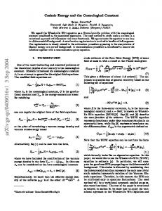
in complete analogy to Sorkin’s proposal in the cosmological context. To summarize, thermal fluctuations of a finite number of molecules in the context of fluid membranes are analogous to quantal fluctuations associated with a finite number of discrete spacetime elements in the causet model of quantum gravity. These fluctuations are finite size effects and dissappear (i.e ∆σ → 0) in the thermodynamic limit (N → ∞) just as in the cosmological context at late epochs Sorkin’s argument predicts that the cosmological constant fluctuations dissappear. Experiments: The fluctuating surface tension of fluid membranes can be experimentally probed. We briefly describe possible experiments in idealised form. Consider a cylindrical fluid membrane in an ambient buffer solution stretched between two tiny (say tens of nanometres) rings. The ends of the cylinder are open so that the pressure on the two sides of the membrane are balanced. One of the rings is attached to a piezoelectric translation stage (figure) which can be moved in nanometre steps. The other ring is attached to a micron sized bead which is confined in an optical trap. If r is the radius of the rings, the area of the membrane is given by 2πrL, where L is the separation between the rings. At fixed separation L, one can measure the force F on the micron sized bead by looking (through a microscope) at its displacement in the optical trap. This force F is related to the surface tension by F = 2πrσ. Thus, one can directly measure the surface tension of a small fluid membrane as a function of its area. We expect to find a small fluctuating component in the surface tension, whose magnitude decreases as the inverse square root of the area of the √ membrane. In order for this 1/ N effect to be appreciable, N has to be suitably small. For a .1% effect we need N = 106 . Variants of this setup [26] can be considered, for example 10
using a strip geometry for the membrane rather than a cylindrical one. One could also let the bead “recoil” by switching off the trap [27]. The experiments proposed above are well within the realm of possibility. In fact similar experiments have already been done (albeit with a completely different motivation). In [27], the authors report an experiment done on vesicles which is similar to the experiment we have proposed. They pull out a tube (80nm radius) of lipid membrane from a multilamellar vesicle of DDAB, stretch it out over tens of microns, and measure its force extension relation. While [27] do measure a surface tension it is not the effect that we discuss here. Kaluza-Klein compactification: One could view the circular cross section of the cylinder as a ‘compactified’ internal dimension. The cylinder can be regarded as a line’s worth of circles. From a coarse perspective one can disregard the compact circular dimension and view the cylinder as a line. From dimensional reduction the line tension gets a contribution from the (extrinsic) curvature of the compactified dimension. The expected value of the surface tension (in order of magnitude) is σ = T /r 2 , where r is the radius of the compact dimension. The measured value [27] of the surface tension ∼ 10−6 N/m (or 10−3 milliJoules per metre squared) agrees in order of magnitude with T /r 2 , where r ∼ 80nm is the radius of the tubule in the experiment. We say a compact dimension is large if its radius is much greater than the molecular scale lmol . Let us define ξ = r/lmol . After dimensional reduction, we find that the predicted √ magnitude for the fluctuating line tension decreases by a factor 1/ ξ. This is in parallel with Sorkin’s observation [12] that in models with large extra dimensions [28] the prediction of a fluctuating cosmological constant results in a magnitude much smaller than the observed one. Conclusion: We have developed an analogy between the surface tension of membranes and the cosmological constant. The analogy is based on the standard mapping between quantum field theory and statistical mechanics. We have shown that the cosmological constant problem has its counterpart in the context of membranes and suggested experimental probes for measuring a fluctuating surface tension thus realising in analogy Sorkin’s proposal 11
of a fluctuating cosmological constant. The main new point of this paper is the connection between two disparate fields. As some aspects are better understood in one field and some in the other, we are able to derive insights from both fields. For example, part b) is discussed in cosmology [7] but we have not seen a corresponding discussion in membranes. The reverse is true for part a) [23]. One could use the analogy to transport this discussion to cosmology. One could invoke an external reservoir to provide causet elements at Planck density. Carrying over ideas from the membrane context, one could introduce in analogy to f (α) a “Quantum action per causet element”, a function of causet four-density which has a minimum at the Planck four density. Both part a) and part b) seem to emerge naturally from this description. We hope to interest the causet community in implementing this idea in technical detail. The free energy of a membrane has a term proportional to the intrinsic curvature, which in two dimensions is purely topological. Such a term can affect the global topology of the membrane. For example a large (negative) value for a′2 favours the production of handles. For instance, the “Plumber’s nightmare phase” in membranes [19] is an example of a phase where there is a proliferation of handles. There are similar effects in the GR context too: there are topological terms which one can add to the action at the next order (after the Einstein-Hilbert term). These would be negligible at ordinary energies and length scales, but at the Planck scale may favour the production of handles, an idea which has been discussed before as “space-time foam”. The analogy we develop in this paper (like all analogies) has its limitations. Obvious differences are those of dimension (two versus four) and signature (Euclidean versus Lorentzian). In the case of Lorentzian space-time the only distribution of causet elements consistent with local Lorentz invariance is Poisson. In the case of membranes, the distribution of amphiphiles on Σ is certainly not Poisson. There are correlations between the √ molecules. In spite of this difference, 1/ N fluctuations of the surface tension arise, due to the central limit theorem. Another important difference is that in GR all the field variables which appear in the action are intrinsic, whereas the membrane free energy has terms 12
dependent on the embedding. One must remember that for finite size systems, the choice of ensemble is crucial. For a discussion of this point and its operational realisation see [29]. Throughout this paper we have worked in the constant area (or Helmholtz) ensemble: we keep the area of the membrane fixed and study the surface tension fluctuations. In the Helmholtz ensemble, we expect to see fluctuations in the surface tension manifesting as fluctuations in the bead about its mean position. In the conjugate Gibbs ensemble where one holds the surface tension constant one would expect to see area fluctuations. In analogy, in the cosmological context, observers are viewing the universe at a particular epoch or fixed 4 volume V (or Helmholtz ensemble). There is no counterpart in cosmology of the Gibbs ensemble, which would involve fixing the cosmological constant and letting the “epoch” fluctuate. We have described a “history” (in analogy to a configuration) as a timeless entity. While this is correct in the mathematical analogy we work with, a history is described in physical terms by its development or unfolding. In causet theories, there are efforts to dynamically describe causets in terms of elements coming into being one at a time. The present description of a “history” as timeless does not capture this unfolding of the causet dynamics. In spite of its limitations, we feel that the analogy we develop here is suggestive and can be fruitfully pursued further. Acknowledgements: We thank S. Surya for discussions on causets and Y. Hatwalne for conversations on fluid membranes. We also thank R. Bandyopadhyay, D. Bhattacharya, R. Capovilla, D. Cho, J. Henson and B. Nath for their comments.
13
FIGURES FIG. 1. Experimental Setup (not to scale) for measurement of the Surface Tension of a Fluid Membrane. The tubular membrane is stretched between two microscopic rings.
14
Table 1: The Analogy Membranes
Universe
Configuration C
History H
Area of a configuration A
Four volume of a history V
Sum over configurations
Sum over histories
Energy E(C)
Classical Action I(H)
Minimum energy configuration
Classical Path Of Least Action
Temperature T
Planck’s constant h ¯
Thermal Fluctuations
Quantum Fluctuations
Surface Tension σ
Cosmological Constant λ
Molecular Length lmol
Planck Length lP lanck
molecules
Causet elements
Free Energy
Quantum Action
R √ E0 = a0 d2 x γ
R √ I0 = c0 d4 x −g
15
E2 =
R
√ d2 x γH 2
R √ I2 = c2 d4 x −gR
Molecular level discreteness of space Planck scale discreteness of spacetime
Plumber’s nightmare phase
Spacetime foam
16
Table 2: Typical Interfacial Tension Values Interfaces
Surface Tension
in milli Joules per metre squared
Water-Vapour
72.6
Water-Oil
57
Mercury-Water
415
Glycerol-Air
63.4
Decane-Air
23.9
Hexadecane-Air
27.6
Octane-Air
21.8
Water-Air
40
17
REFERENCES [1] W. Unruh, Phys. Rev. Lett. 46, 1351 (1981); Phys. Rev. D51, 2827 (1995). [2] C. Barcela, S. Liberati and M. Visser, Living Reviews in Relativity, 8, 12 (2005) and references therein. [3] See for instance, G. E. Volovik, The Universe in a Helium Droplet, Clarendon Press, Oxford (2003); Artificial Black Holes, ed. M. Novello, M. Visser and G. Volovik, World Scientific, Singapore (2002). [4] M. J. Bowick, L. Chandar, E. A. Schiff and A. M. Srivastava, Science, 263, 943 (1994), R. Ray and A. M. Srivastava, Physical Review, D69, 103525 (2004). [5] See for instance, Cosmic Strings and other topological defects, A. Vilenkin and E. P. S. Shellard, Cambridge University Press, Cambridge 1994, T. Vachaspati and A. Vilenkin, Physical Review, D30, 2036 (1984). [6] R. Capovilla, J. Guven and E. Rojas, cond-mat/0505631 and references therein. [7] R. D. Sorkin, “First Steps With Causal Sets”, in General Relativity and Gravitational Physics Proceedings of the Ninth Italian Conference on GR and Gravitational Physics, Capri, Italy, September 1990 ( R. Ciani, R de Ritis, M. Francaviglia, G. Marmo, C. Rubano and P. Scudellaro, eds.), pp 68-70, World Scientific, Singapore, 1991. R. D. Sorkin, Int. J. Th. Phys. 36 2759 (1997) and references therein; M. Ahmed, S. Dodelson, P. Greene and R. D. Sorkin, Physical Review D69 103523 (2004). [8] A similar problem faced the learned men of Brobdingnag when confronted with Gulliver, who was tiny by the standards of Brobdingnag. Why was he so small and why (if he was so small) did he exist at all? [9] A. G. Riess et al, Astrophys. J 116, 1009 (1998); S. Perlmutter et al, Astrophys. J 517, 565 (1999).
18
[10] For instance “quintessence models” suffer from the “why now?” problem [7]. They need an energy scale of h ¯ H0 ∼ 10−33 eV to turn on the field at the present epoch. H0 here is the Hubble constant. [11] Causal Sets: Discrete Gravity by R.D. Sorkin, in Lectures on quantum gravity, Eds A. Gomberoff and D. Marolf, Springer, N.Y. (2005). [12] R. D. Sorkin, gr-qc/0503057. [13] A. Einstein, Siz. Preuss. Acad. Scis. (1919). [14] S. Weinberg, Rev. Mod. Phys. 61, 1 (1989). [15] W. G. Unruh Physical Review D40 1048 (1989); W. G. Unruh and R. W. Wald Physical Review D40 2598 (1989). [16] T. Padmanabhan, Classical and Quantum Gravity 19, L167 (2002). [17] G. E. Volovik, gr-qc/0406005. [18] Statistical mechanics of membranes and surfaces, eds. D. Nelson, S. Weinberg and T. Piran, World Scientific, Singapore (2004). [19] Soft Matter Physics, M. Daoud and C. E. Williams, Springer-Verlag, Berlin (1999). [20] F. Dowker, J. Henson and R. D. Sorkin, gr-qc/0311055. [21] For instance, the symmetry of the bilayer prevents spontaneous curvature terms (like R
Σ
H) from being generated.
[22] In this case the molecular scale is set by the thickness of the bilayer, which is related to the length of the surfactant molecules. [23] Z.G. Wang and S.A. Safran, J. Phys. (France), 51 185 (1990); Statistical Thermodynamics of Surfaces, Interfaces and Membranes, Samuel A. Safran, Addison-Wesley, (1994), Reading, Massachussetts.
19
[24] Basic Concepts For Simple And Complex Liquids, J. L. Barrat and J. P. Hansen, Cambridge University Press (2003). [25] It would be interesting to study the renormalisation group flow of the fluid membrane surface tension as in (3,4). There has been some work along these lines (F. Brochard, P. G. de Gennes and P. Pfeuty, J. de Phys. (France) 37, 1099), whose implications in the present context are not clear. Our argument deals with a finite number of molecules, and does not require renormalisation. [26] For example, surface tension fluctuations of micron sized vesicles may be observable as shape fluctuations by light scattering. [27] T. Roopa, G. V. Shivashankar, Applied Physics Letters 82, 1631 (2003) and references therein. [28] L. Randall and R. Sundrum, Phys. Rev. Lett, 83, 3370, 4690 (1999). [29] S. Sinha and J. Samuel Physical Review E71, 021104 (2005).
20