Also, Gsym has a weight function w : Venvâªsys ÃVenvâªsys â Zâª{â¥} that .... Negative weights whenever the elevator is not on the requested floor ... 14) and source floor and destination floor do not change while requests are pending (l. 16).
Symbolic BDD and ADD Algorithms for Energy Games Shahar Maoz
Or Pistiner
Jan Oliver Ringert
School of Computer Science Tel Aviv University, Israel
Energy games, which model quantitative consumption of a limited resource, e.g., time or energy, play a central role in quantitative models for reactive systems. Reactive synthesis constructs a controller which satisfies a given specification, if one exists. For energy games a synthesized controller ensures to satisfy not only the safety constraints of the specification but also the quantitative constraints expressed in the energy game. A symbolic algorithm for energy games, recently presented by Chatterjee et al. [9], is symbolic in its representation of quantitative values but concrete in the representation of game states and transitions. In this paper we present an algorithm that is symbolic both in the quantitative values and in the underlying game representation. We have implemented our algorithm using two different symbolic representations for reactive games, Binary Decision Diagrams (BDD) and Algebraic Decision Diagrams (ADD). We investigate the commonalities and differences of the two implementations and compare their running times on specifications of energy games.
1
Introduction
Reactive synthesis is an automated procedure to obtain a correct-by-construction reactive system from its temporal logic specification [17]. Rather than manually constructing a system and using model checking to verify its compliance with its specification, synthesis offers an approach where a correct implementation of the system is automatically obtained, if such an implementation exists. Traditionally, specifications for synthesis express qualitative properties of desired system behavior, which are either satisfied or not satisfied. Over the last decade interest has increased for quantitative properties [2], which can express, e.g., cost of actions or probability of success, and allow for synthesis of optimal solutions. One intuitive and popular quantitative extension of games for reactive synthesis are energy games (EGs), defined by Bouyer et al. [5], which model quantitative consumption of a limited resource, e.g., cost, time, or energy. Transitions between states are annotated with weights. A play starts with a finite energy level that is updated by the weight on every transition. An infinite play is winning for the system if the energy level never goes below 0. The EG is realizable if the system has a strategy to win for initial choices of the environment. The objective of synthesis for EG is to construct such a strategy. Brim et al. [6] have presented an efficient pseudo-polynomial algorithm for solving EGs (polynomial in the state space and the maximal weight). The algorithm is bounded by the maximal initial energy. Because the maximal initial energy for realizable energy games is bounded the algorithm is complete. It computes the minimal energy required to win from any state in a backwards manner, using a fixed point calculation. A representation by minimal energy levels is symbolic in the sense of antichains [11], also used in the algorithm of Chatterjee et al. [9]. These algorithms are thus symbolic in the quantitative values but concrete in the representation of game states and transitions. In this work we present a novel algorithm that is optimized for reactive energy games and symbolic both in the quantitative values and in the underlying game representation. Our algorithm implements a fixed point computation similar to Chatterjee et al. [9] but due to the reactive nature of the game it updates energy levels of system and environment states in one instead of two steps. Our symbolic
To appear in EPTCS.
c S. Maoz & O. Pistiner & J.O. Ringert
This work is licensed under the Creative Commons Attribution License.
2
Symbolic BDD and ADD Algorithms for Energy Games
algorithm also uses antichains. However, the antichains are now defined over sets of states and their sets of energy levels instead of over single states and their sets of energy levels. These modifications require efficient symbolic data structures and corresponding operations to represent the (intermediate) results of the fixed point computation. We further present two different implementations of our algorithm. The first implementation is based on Binary Decision Diagrams (BDDs) [7] to represent states, transitions, and weight definitions. Antichains are then maps mapping minimal energy levels to BDDs. Accordingly, the fixed point calculation of the algorithm is based on iterations over minimal energy levels and weights and is executed using symbolic BDD operations. Our second implementation is based on Algebraic Decision Diagrams (ADDs) [1], a special case of Multi-Terminal Binary Decision Diagrams (MTBDDs) [13]. ADDs have numbers as terminal nodes — instead of TRUE and FALSE in the case of BDDs — and provide efficient implementations of symbolic algebraic operations. With ADDs, an antichain in our algorithm is expressed in a single ADD. Again, we have implemented the fixed point calculation of the algorithm using only symbolic ADD operations. The ADD and BDD algorithms do not only use symbolic data structures for efficient representation: contributions of our implementations are also their specific use of symbolic manipulations for efficiently performing quantitative operations. We explain both implementations to highlight their commonalities and differences. In Sect. 7 we compare the running times of the BDD and ADD implementations against each other and against themselves over increasing sizes of specifications and different specifications of weights. We present background on games, BDDs, ADDs, and EGs in Sect. 2. Sect. 3 introduces a running example specification. We present our generic algorithm in Sect. 4, and its BDD and ADD implementations in Sect. 5 and Sect. 6 resp. Sect. 7 presents a preliminary evaluation of our two implementations. We discuss the results and related work in Sect. 8 and conclude in Sect. 9.
2 2.1
Preliminaries Infinite Games, BDDs, ADDs
We repeat some basic definitions of games, BDDs, and ADDs. We also describe the general approach for symbolically representing games between an environment and a system player using BDDs.
Games, game graphs, plays, and strategies We consider infinite games played between two players on a finite directed graph as they move along its edges. For a game we define a game graph as a tuple Γ = hG = hV, E, wi,V0 ,V1 i, where G = hV, E, wi is a finite directed graph with a weight function w : E → Z that attaches weights to its edges. V0 ,V1 is a partition of V into V0 , the set of player-0 (the maximizer) vertices, and V1 , the set of player-1 (the minimizer) vertices. Each vertex v ∈ V has out degree at least one, i.e., G has no deadlocks. A play starts by placing a pebble on a given initial vertex, and continues infinitely many rounds as the two players move the pebble along the edges of G. In each round, if the pebble is on a vertex v ∈ Vi , i ∈ {0, 1}, then player-i chooses an outgoing edge from v to some adjacent vertex u ∈ V , and the next round starts with the pebble on u. The infinite path formed by the rounds is called a play. A strategy of player-i is a function that given the prefix of a play ending in a vertex of player-i returns a successor vertex.
S. Maoz & O. Pistiner & J.O. Ringert
3
Binary Decision Diagrams and Algebraic Decision Diagrams Binary decision diagrams (BDDs) [7] are a compact data structure for representing and manipulating Boolean functions. For the purpose of verification and synthesis they are usually used to represent sets of Boolean vectors [14], e.g., encoding sets of states or transitions. Bryant [7] showed how Boolean operations on BDDs can be efficiently implemented, including logical connectives and existential and universal abstractions. ADDs [1] are a generalization of BDDs, such that the terminal nodes may take on values belonging to a set of constants different from 0 and 1, such as integers or reals. Another name for ADDs is Multi-Terminal Binary Decision Diagrams (MTBDDs) [13], which reflects their structure rather than their application for computations in algebras. An ADD represents a Boolean function of n variables f : {0, 1}n → S where S is a set of constants. Boolean, arithmetic, and abstraction operations are all applicable to ADDs. We now briefly state the most important operations that we use in our ADD based algorithm. For ADDs g, h, and a 0-1 ADD f , arithmetic operators op ∈ {+, −, ·, max, . . .}, denoted g op h, operate on the terminal nodes for common variable assignments, the If-then-else Boolean operation is defined as ITE( f , g, h) = f · g + ¬ f · h , and abstraction of variables v from g, which aggregate terminal values of g for all assignments to variables in v by operators min or max.
Symbolic representation of game graphs for reactive games Reactive games are turn-based two players games, between an environment and a system player, in which the environment always plays first and the system reacts. The environment controls the input variables, denoted by env, and the system controls the output variables, denoted by sys, all are assumed to be Boolean, such that their values are modified in each step of the game [17]. We denote by Vvar := {0, 1}var all the possible assignments to the variables var, where svar ∈ Vvar is some assignment to var. We now define the symbolic weighted game graph Gsym := hθ e , θ s , ρ e , ρ s , wi for reactive games. A state s in Gsym is an assignment to all variables, i.e., s := senv∪sys ∈ Venv∪sys . That means each state belongs to both players (unlike the general model). We denote by θ e , θ s the sets of initial states of the environment and the system, respectively. Each is represented by a BDD (or by a 0-1 ADD) that encodes its characteristic function: χθ e : Venv → {0, 1} and χθ s : Venv∪sys → {0, 1}. Each player has a transition relation that defines its valid transitions in Gsym . It is denoted by ρ e and ρ s for the environment and the system, respectively. A next state in Gsym , as opposed to a current state, is represented by a primed version of the variables sys0 and env0 . Therefore, the BDDs (or 0-1 ADDs) that represent ρ e and ρ s encode the characteristic functions χρ e : Venv∪sys∪env0 → {0, 1} and χρ s : Venv∪sys∪env0 ∪sys0 → {0, 1}. The bijection prime : Vsys∪env → Vsys0 ∪env0 replaces unprimed variables by their primed counterparts. We denote a transition from state s1 to state s2 by ts1 ,s2 := s1 ∪ prime(s2 ) ∈ Venv∪sys∪env0 ∪sys0 . It is valid if ts1 ,s2 ∈ ρ e ∩ ρ s , thus consists of a valid transition for environment choice se2 := senv ∈ Venv , denoted by ts1 ,se2 := s1 ∪ prime(se2 ) ∈ ρ e , followed by a valid transition for system choice ss2 := ssys ∈ Vsys , denoted by ts1 ,se2 ,ss2 := s1 ∪ prime(se2 ) ∪ prime(ss2 ) ∈ ρ s . Also, Gsym has a weight function w : Venv∪sys × Venv∪sys → Z ∪ {⊥} that attaches weights to its transitions, such that for all pairs of states s1 , s2 if ts1 ,s2 ∈ ρ e ∩ ρ s , w(s1 , s2 ) ∈ Z, and otherwise, w(s1 , s2 ) =⊥. For details of its actual representation see Sect. 5 and Sect. 6.
Notation We work with abstractions where a BDD represents a set of states or transitions, i.e., BDD ≡ Set of States or BDD ≡ Set of Transitions. An ADD represents a function assigning an integer, plus or minus infinity, to every state or transition, i.e., ADD ≡ States → Z±∞ or ADD ≡ Transitions → Z±∞ .
4
2.2
Symbolic BDD and ADD Algorithms for Energy Games
Energy Games
Energy games (EG), also called the lower bound problem, have been studied by Bouyer et al.[5]. We give the formal definitions of EG as defined in [5, 6], followed by a fixed point formulation of the solution for EG as in [5, 9]. EG definition and objectives We add to an infinite play on an EG graph Γ an initial credit or initial energy value c ∈ N. We define the energy level of the prefix v0 v1 . . . v j of the play p = v0 v1 . . . v j . . ., by j−1 EL(p, j) = c + ∑i=0 w(vi , vi+1 ). The objective of player-0 is to construct an infinite play p = v0 v1 . . . v j . . . such that the energy level is always non-negative during the play, i.e., EL(p, j) ≥ 0 f or all j ≥ 1. We say that such a play p is winning for player-0. Otherwise, if the energy level goes below zero during p, it is winning for player-1. Given an initial credit c, a strategy is winning for player-0 from v ∈ V for c if all plays resulting from the strategy are winning for player-0. A vertex v is winning for player-i if there exists a winning strategy for player-i from v for some initial credit c. We consider two EG problems: (1) Decision problem: Given a vertex v, the problem asks if there exists an initial amount of energy that suffices for player-0 to win from v; and (2) Minimum credit problem: which asks for every vertex v ∈ V , what is the minimal initial amount of energy that suffices for player-0 to win from v. A solution of the second also provides a solution for the first by checking whether the minimal initial energy is finite. In addition a solution for the second allows for the construction of optimal memoryless strategies for solving EGs [9]. We thus focus on the minimum credit problem. Algorithm for solving energy games from [9] Both Chatterjee et al. [9] and Bouyer et al. [5] present algorithms to solve the minimal credit problem of EGs. Their solutions are presented as the greatest fixed point of a monotone operator on a power set lattice. Given an EG graph Γ = hG = hStates, E, wi, States0 , States1 i and a bound c ∈ N, we denote by SE(c) the pairs of states and energy values up to c, i.e., States × {n ∈ N | n ≤ c}. We relate to the monotone bounded operator Cprec : P(SE(c)) → P(SE(c)), where P(SE(c)) is the power set of SE(c), that is defined in [9, Eqn. 1]. Chatterjee et al. [9] present a symbolic fixed point algorithm that computes a set of pairs consisting of a state and an energy level that suffices for player-0 to win for that state. It performs iterative applications of Cprec to SE(c), which results in a finite ⊆-descending chain whose last element approximates the greatest fixed point of Cprec . Symbolic representation of upward closed sets We define a partial order � ⊆ SE(c) × SE(c) (i.e., reflexive, transitive, antisymmetric binary relation), such that for all (s, e), (s0 , e0 ) ∈ SE(c), (s, e) � (s0 , e0 ) iff s = s0 ∧ e ≤ e0 . We call Up(�, A) := {(s, e) ∈ SE(c) | ∃(s0 , e0 ) ∈ A : (s0 , e0 ) � (s, e)} the � -upward closure of A ⊆ SE(c). A set A ⊆ SE(c) is �-upward-closed if for all (s, e), (s0 , e0 ) ∈ SE(c), if (s, e) ∈ A and (s, e) � (s0 , e0 ), then (s0 , e0 ) ∈ A. An �-upward-closed set equals its upward closure. We denote by Min(�, A) the minimal elements of A, formally Min(�, A) := {(s, e) ∈ A | ∀(s0 , e0 ) ∈ A : (s0 , e0 ) � (s, e) ⇒ (s0 , e0 ) = (s, e)}. A set A ⊆ SE(c) is an antichain if all pairs (s, e) 6= (s0 , e0 ) ∈ A are �-incomparable. An �-upward-closed set is symbolically represented by its minimal elements, as the former is uniquely determined by the latter: if A ⊆ SE(c) is an upward closed set, then Up(�, Min(�, A)) = A. Description of the algorithm from [9] by operations on antichains Bouyer et al. [5] present an alternative description to the fixed point solution in terms of sufficient infimum credits. Since every element U of the Cprec application from [9, Eqn.1] is �-upward-closed, it can be symbolically represented by the antichain Min(�,U) [9]. For a bound c ∈ N the bounded operator CpreMinc : A(SE(c)) → A(SE(c)),
S. Maoz & O. Pistiner & J.O. Ringert
5
where A(SE(c)) is the set of antichains of SE(c), is defined by: εmin (Λ) = {(s0 , e0 ) ∈ SE(c) | s0 ∈ States0 ∧ e0 =
ηmin (Λ) = {(s1 , e1 ) ∈ SE(c) | s1 ∈ States1 ∧ e1 =
min
[ max(0, e1 − w(s0 , s)) ]}
(1)
max
[ max(0, e0 − w(s1 , s)) ]}
(2)
(s0 ,s)∈E s.t. ∃e1 (s,e1 )∈Λ
(s1 ,s)∈E s.t. ∃e0 (s,e0 )∈Λ
CpreMinc (Λ) = Min(�, εmin (Λ) ∪ ηmin (Λ)) = εmin (Λ) ∪ ηmin (Λ)
(3)
CpreMinc is used to compute the sets of pairs consisting of a state and the minimal initial energy that suffices for player-0 to win for that state. For every pair of antichains A, B ∈ A(SE(c)), we define the partial order v such that A v B iff ∀(sb , eb ) ∈ B ∃(sa , ea ) ∈ A such that (sa , ea ) � (sb , eb ). Note that A v B iff Up(�, B) ⊆ Up(�, A). CpreMinc is a monotone operator over the complete lattice (A(SE(c)), v , 0, / {(s, 0) | s ∈ States})1 . Therefore, there exists a least fixed point of CpreMinc in this lattice that can be calculated by iterated applications of CpreMinc to the antichain ZS = {(s, 0) | s ∈ States}. ZS assigns every state 0 initial energy, which is the minimal initial energy that is sufficient for player-0 to win a 0 steps game. In general, if Λ contains states and minimal energy levels for player-0 to win in k steps, then CpreMinc (Λ) contains those required for k + 1 steps.
3
Example Specification: Elevator
We present an example specification of a controller for an elevator servicing multiple floors. The environment inputs are pending requests to floors and the current floor of the cabin. The controller outputs are commands for moving up, stopping, or moving down. Quantitative properties of the specification are expressed as weights on transitions. Negative weights whenever the elevator is not on the requested floor and positive weights for reaching a requested floor. Reactive specification The elevator specification is shown in List. 1. The environment controls the variable pending which signals a request of the elevator cabin to a destination floor given by the variable dest floor. The environment also maintains variables to keep track of the source floor src floor (location of cabin when request arrived) and the current floor current floor. The system controls the variable move with the possible moves of the cabin (l. 7). The specification in List. 1 defines two abbreviations TOP for the top floor and THERE for the condition that the current floor is the requested destination floor. The remainder of the specification defines from l. 13 to l. 26 safety constraints for the environment, i.e., assumptions, and from l. 28 to l. 31 safety constraints for the system, i.e., guarantees. Some important assumptions regard the values of variables storing the source floor: the value of source floor is the current floor when a request is issued (l. 14) and source floor and destination floor do not change while requests are pending (l. 16). Requests are disabled when the destination floor is reached (l. 18). The assumptions in l. 21 to l. 26 ensure that the environment sets the current floor according to the move commands of the system. The safety constraints for the system ensure that the cabin does not move up on the top floor (l. 29) and that it does not move down on the bottom floor (l. 31). 1 For
every M ⊆ A(SE(c)), inf M := Min(�, M), sup M := Min(�, S
T
m∈M Up(�, m)).
For details and proofs see [10].
6 1 2 3 4 5 6 7
Symbolic BDD and ADD Algorithms for Energy Games VARENV pending : boolean; src_floor : 0..4; dest_floor : 0..4; current_floor : 0..4; VAR move : {UP, DOWN, STOP};
8 9 10 11
DEFINE TOP := 4; THERE := current_floor = dest_floor;
12 13 14 15 16 17 18 19 20 21 22 23 24 25 26
ASSUMPTION -- set src_floor G (!pending & next(pending) -> next(src_floor) = next(current_floor)); ASSUMPTION -- remember src_floor and dest_floor G (pending -> (next(src_floor) = src_floor & next(dest_floor) = dest_floor)); ASSUMPTION -- keep requests pending G (pending & !THERE -> next(pending)); ASSUMPTION -- disable requests G(THERE & pending -> next(!pending)); ASSUMPTION -- do go up G (move=UP & current_floor < TOP -> next(current_floor) = current_floor + 1); ASSUMPTION -- do stop G (move=STOP -> next(current_floor) = current_floor); ASSUMPTION -- do go down G (move=DOWN & current_floor > 0 -> next(current_floor) = current_floor - 1);
27 28 29 30 31
GUARANTEE -- don’t G (current_floor GUARANTEE -- don’t G (current_floor
go up on top floor = TOP -> move!=UP); go down on bottom floor = 0 -> move!=DOWN);
Listing 1: A specification for an elevator controller consisting of environment variables VARENV, system variables VAR, definitions DEFINE, assumptions ASSUMPTION, and guarantees GUARANTEE
Symbolic elevator game graph The assumptions and guarantees in List. 1 describe the game graph for a reactive game in terms of initial states of the environment θ e and system θ s and the transitions of the environment ρ e and system ρ s . The conjunction of all assumptions without the temporal operator G defines θ e while the conjunction of all guarantees without the temporal operator G defines θ s . In the example of List. 1 we have no such assumptions or guarantees and thus θ e ≡ TRUE ≡ θ s . Similarly, the conjunction of all assumptions with the temporal operator G defines ρ e while the conjunction of all guarantees with the temporal operator G defines ρ s . The two guarantees in List. 1, ll. 28-31 express that ρ s evaluates to FALSE for all states with current floor=TOP & move=UP or current floor=0 & move=DOWN, i.e., these states are deadlocks for the system. A state in the game graph is an assignment to all variables, e.g, s1 =(pending=true, src floor=1, dest floor=4, current floor=1, move=DOWN). From this state the assignments to environment variables in successor states are determined by the transition relation ρ e and the assignment to system variable move is restricted by the transition relation ρ s to either STOP or UP leading to two possible successor states of s1 . The number of reachable states in the game graph is 750. For 10 floors the number of reachable states is 6,000 and for 50 floors the number of reachable states is 750,000.
S. Maoz & O. Pistiner & J.O. Ringert 1 2 3 4 5 6 7 8 9 10
WEIGHT: 1 pending & WEIGHT: 2 pending & WEIGHT: 3 pending & WEIGHT: 4 pending & WEIGHT: -1 pending &
7
next(!pending) & abs(src_floor - dest_floor) = 1; next(!pending) & abs(src_floor - dest_floor) = 2; next(!pending) & abs(src_floor - dest_floor) = 3; next(!pending) & abs(src_floor - dest_floor) = 4; !THERE;
Listing 2: A weight definition for transitions of the elevator with reward for reaching a floor depending on the distance traveled (between 0 and 4) and punishment -1 for not being at the requested floor. Five entries define six weights -1, 0, 1, 2, 3, and 4 1 2 3 4
WEIGHT: 1 pending & THERE; WEIGHT: -1 pending & !THERE;
Listing 3: Weight definition for transitions of the elevator with reward 1 for reaching a requested floor and punishment -1 for not being at the requested floor. Two entries define three weights -1, 0, 1 Weight definitions List. 2 shows a definition of weights for transitions of the elevator. Every weights definition entry starts with keyword WEIGHT and the value of the weight followed by an LTL formula characterizing a set of transitions. As an example, the first entry in List. 2 defines weight 1 for transitions from states with a pending request and absolute difference abs (src floor-dest floor) = 1 to states with the request disabled. As another example, the last entry in List. 2 defines weight -1 for all transitions from states where a request is pending and the cabin is not at the destination floor. Intuitively, the weight definition of List. 2 expresses positive weights per distance traveled. We also present an alternative weight definition in List. 3 consisting of two entries only. The first entry defines weight 1 for all transitions leaving states where a request is pending and the cabin is at the destination floor (l. 2). The second entry defines weight -1 for transitions from states with pending request where the cabin is not at the requested floor. If a transition between states satisfies multiple weight definitions the values of all weights for the transition are added, e.g., a transition that satisfies both the formula in line 8 for weight 4 and the formula in line 10 for weight -1 in List. 2 has weight 3. In case a transition does not satisfy any of the weight formulas it is assigned the default weight 0, e.g., all transitions from states where no requests are pending in the weight definition of List. 3. The addition of weights for overlapping sets of transitions and the completion with 0 is a preprocessing step. This means that the weights definition in List. 2 does not define 5 weights (number of WEIGHT entries) but 6 weights (including weight 0 for transitions defined both in line 2 and line 10). The weights definition in List. 3 defines 3 weights of values -1, 0, and 1. When referring to the number of weights, e.g., to describe the complexity of the algorithm the number of weights is the resulting number of non-overlapping weights and not the number of entries in our declarative weights specification. Elevator energy game and initial energy The safety constraints of the system and environment in List. 1 together with the weight definition in List. 2 or List. 3 define an energy game. Intuitively, in an energy game the system starts with a finite amount of energy and has to make sure that in an infinite
8
Symbolic BDD and ADD Algorithms for Energy Games
play the accumulated energy does never drop below 0. The accumulated energy is defined based on the weights of transitions: for every combined step of the environment and the system (input and output) the weight definition defines an update of the energy level by adding the weight value. For the first weights definition shown in List. 2 the system can win the energy game with a finite initial energy. An obvious strategy is to always immediately move to a floor once it is requested by the environment. The accumulated negative weights -1 for pending requests will then be compensated by the weight for reaching the destination floor. Interestingly, the elevator can do even better in terms of minimal energy levels. The highest minimal required initial energy from any state is 7. One such worst-case state is (pending=true, src floor=4, dest floor=4, current floor=1, move=DOWN). In this state the cabin is on floor 1 but travels to floor 0 while the environment issued a request to the top floor.2 The top floor can be reached within 5 steps (accumulated energy level 7-5=2). The reward for reaching the floor is 0 because src floor = dest floor (note that this reward is obtained on outgoing transitions). The cabin immediately travels to floor 3 where no request is pending (see assumption in List. 1, l. 20). It then arrives at floor 2 still with energy level 2 (because no request was pending on floor 3) and can now reach all floors within two steps and thus maintaining at least 0 energy. For the alternative weights definition shown in List. 3 the system cannot win for any finite initial energy. From the above example strategy it is clear that with weight 2 instead of 1 in List. 3, l. 1 the system could win the energy game3 .
4
Our Symbolic Algorithm
We start with a description of our reactive EG model in terms of the general model of EG, both presented in Sect. 2, where player-0 (maximizer) is the system and player-1 (minimizer) is the environment. Such a description shows that our model is an instance of the general model despite their differences. We then proceed with the presentation of a generic version of our symbolic algorithm for reactive EG.
4.1
Model of Reactive Energy Games
Formally, we show a reduction that takes as input a symbolic game graph Gsym = hθ e , θ s , ρ e , ρ s , wi for reactive EG as defined in Sect. 2, and outputs a bipartite game graph ΓR = hGR = hV R , E R , wR i,V0R ,V1R i for EG. We start by defining two sub graphs of GR , each consists of a simple cycle C such that if any of its vertices is reached during a play then the players are trapped in C indefinitely. (1) Cwin : a (+1) R win R win win win R win weight cycle formed by the vertices vwin 0 ∈ V0 , v1 ∈ V1 , and the edges e0 = (v0 v1 ) ∈ E , e1 = win win R R win R win loss (v1 v0 ) ∈ E such that w (e0 ) = 1, w (e1 ) = 0. (2) C : a (−1) weight cycle formed by the loss loss R R loss R loss loss loss R loss vertices vloss 0 ∈ V0 , v1 ∈ V1 , and the edges e0 = (v0 v1 ) ∈ E , e1 = (v1 v0 ) ∈ E such that R loss wR (eloss 0 ) = (−1), w (e1 ) = 0. R Γ is constructed by the following two phases: (1) Takes hθ e , θ s i as inputs: we add an initial vertex v0/ ∈ V1R that corresponds to V0/ , i.e., all variables have no values assigned. In case there are no valid initial states for the environment, i.e., θ e = 0, / thus all plays on Gsym are winning for the system, we win R R add e = (v0/ , v0 ) ∈ E with w (e) = 0 leading to Cwin , and output ΓR . Otherwise, for every initial state se ∈ θ e we add a vertex vse ∈ V0R and an edge e = (v0/ , vse ) ∈ E R such that wR (e) = 0, whereas for every s ∈ θ e ∩ θ s where s = se ∪ ss we add a vertex vs ∈ V1R and an edge e = (vse , vs ) ∈ E R with wR (e) = 0. 2 Note
that this initial state is not required for winning because the system could choose move=UP but it represents an interesting worst-case energy level. 3 This non-trivial strategy for winning with at most weight 2 for 5 floors was indeed found by our implementation.
S. Maoz & O. Pistiner & J.O. Ringert
9
For every se ∈ θ e such that for all ss ∈ Vsys , se ∪ ss ∈ / θ s , i.e., an initial state which is a deadlock for the R R loss system, we add e = (vse , v1 ) ∈ E with w (e) = (−1) leading to Closs . (2) Takes hρ e , ρ s , wi as inputs: for every valid environment transition ts1 ,se2 ∈ ρ e , we add vs1 ∈ V1R , vts ,se ∈ V0R and e = (vs1 , vts ,se ) ∈ E R 1 2
1 2
with wR (e) = 0. For every ts1 ,se2 ∈ ρ e such that for all system choices ss2 , ts1 ,se2 ,ss2 ∈ / ρ s , i.e., it is a deadlock R R loss . For every t e ∈ ρ e and for the system, we add e = (vts ,se , vloss s1 ,s2 1 ) ∈ E with w (e) = (−1) leading to C 1 2 s s system choice s2 such that ts1 ,se2 ,ss2 ∈ ρ , which results in a valid transition ts1 ,s2 ∈ ρ e ∩ ρ s for both players, we add vs2 ∈ V1R and e = (vts ,se , vs2 ) ∈ E R with wR (e) = w(s1 , s2 ). For every state s1 with vs1 ∈ V1R 1 2 such that for all environment choices se2 , ts1 ,se2 ∈ / ρ e , i.e., a deadlock state for the environment, we add win R R e = (vs1 , v0 ) ∈ E with w (e) = 0 leading to Cwin . ΓR has the following properties: win ω Lemma 1. Given an initial credit c ∈ N, θ e = 0/ if, and only if for all EG plays p on ΓR , p = v0/ (vwin 0 v1 ) , and for all k ≥ 1, EL(p, k) ≥ 0.
Lemma 2. se ∈ θ e is an initial deadlock state for the system if, and only if vse ∈ V0R has one outgoing R loss and there is no initial energy value c ∈ N sufficient for player-0 (-1) weighted edge to vloss 1 ∈ V1 in C R to win from v0/ ∈ V1 . Lemma 3. s ∈ θ e ∩ θ s is an initial deadlock state for the environment in Gsym if, and only if vs ∈ V1R R win and every initial energy value c ∈ N suffices for has one outgoing 0 weighted edge to vwin 0 ∈ V0 in C player-0 to win from vs . Lemma 4. A valid transition from s1 for environment choice se2 , ts1 ,se2 ∈ ρ e , is a deadlock for the system R loss and there is no initial if, and only if vts ,se ∈ V0R has one outgoing (-1) weighted edge to vloss 1 ∈ V1 in C 1 2
energy value c ∈ N sufficient for player-0 to win from vs1 ∈ V1R . Lemma 5. s2 is a deadlock state for the environment in Gsym with a predecessor state s1 such that R win and every ts1 ,s2 ∈ ρ e ∩ ρ s if, and only if vs2 ∈ V1R has one outgoing 0 weighted edge to vwin 0 ∈ V0 in C initial energy value c ∈ N suffices for player-0 to win from vs2 . Lemma 6. A play on Gsym starts at s ∈ θ e ∩ θ s if, and only if a play on ΓR starts with the traversal of e1 = (v0/ , vse ) ∈ E R by player-1 and e0 = (vse , vs ) ∈ E R by player-0, with wR (e1 ) = wR (e0 ) = 0. Lemma 7. A valid W ∈ Z weighted transition for both players from s1 to s2 , i.e., ts1 ,s2 ∈ ρ e ∩ ρ s , is taken at step j ∈ N of a play psym on Gsym if, and only if at step 2 j + 2 of a play p on ΓR player-1 traverses e1 = (vs1 , vts ,se ) ∈ E R and player-0 traverses e0 = (vts ,se , vs2 ) ∈ E R such that wR (e1 ) = 0 and wR (e0 ) = W . 1 2
1 2
4
Theorem 1. Given an initial credit c ∈ N, for all j ≥ 1, e ∈ Z, there exists an infinite reactive EG play psym = s0 s1 . . . s j−1 s j . . . on Gsym with EL(psym , j) = e if, and only if there exists an EG play p = v0/ vse0 vs0 vts ,se vs1 . . . vs j−1 vts ,se vs j . . . = v0 v1 v2 v3 v4 . . . v2 j v2 j+1 v2 j+2 . . . on ΓR with EL(p, 2 + 2 j) = e. 0 1
j−1 j
Theorem 2. 4 Given an initial credit c ∈ N, for all e ∈ N, n ∈ N, 1 ≤ j ≤ n, there exists a finite winning reactive EG play psym on Gsym that ends with a deadlock for the environment, psym = s0 s1 . . . sn−1 sn , with win ω EL(psym , j) = e if, and only if there exists an EG play p = v0/ vse0 vs0 vts ,se vs1 . . . vsn−1 vts ,sen vsn (vwin 0 v1 ) 0 1
n−1
win ω R =v0 v1 v2 v3 v4 . . . v2n v2n+1 v2n+2 (vwin 0 v1 ) on Γ with EL(p, 2 + 2 j) = e and for all k ≥ 1, EL(p, k) ≥ 0.
Theorem 3. 4 Given an initial credit c ∈ N, there exists a finite losing reactive EG play psym on Gsym that ends with se ∈ θ e which is a deadlock for the system, psym = se , if, and only if there exists an EG loss ω R play p = v0/ vse (vloss 1 v0 ) on Γ , and there exists k ≥ 1 such that EL(p, k) < 0. 4 We
omit the proof from this submission.
10
Symbolic BDD and ADD Algorithms for Energy Games
Theorem 4. 4 Given an initial credit c ∈ N, for all e ∈ Z, n ∈ N, 1 ≤ j < n, there exists a finite losing reactive EG play psym on Gsym that ends with a deadlock for the system, psym = s0 s1 . . . sn−1 sen , with loss ω EL(psym , j) = e if, and only if there exists an EG play p = v0/ vse0 vs0 vts ,se vs1 . . . vsn−1 vts ,sen (vloss 1 v0 ) = 0 1
n−1
loss ω v0 v1 v2 v3 v4 . . . v2n v2n+1 (vloss 1 v0 ) with EL(p, 2 + 2 j) = e, and there exists k ≥ 1 such that EL(p, k) < 0.
From Lem. 1 - 5 we get that ΓR has no deadlocks, and conclude from Thm. 1 - 4 that every EG play on ΓR is infinite, therefore compliant with the general model of EG. Moreover, by Thm. 1 every play on ΓR in which neither Closs nor Cwin are visited, determines a reactive play on Gsym with the same energy levels, and vice versa. From Thm. 2 and Lem. 1, 3, 5 we get that every EG (winning) play on ΓR that visits Cwin determines a finite (winning) play on Gsym that ends with a deadlock for the environment. From Thm. 3, 4 and Lem. 2, 4 we get that every EG play on ΓR that visits Closs is losing for the system, and it determines a finite losing game on Gsym that ends with a deadlock for the system. Thm. 1 - 4 focus on the energy levels of player-1’s vertices in ΓR , which are the ones of interest for our reactive EG, and imply that an initial energy level c ∈ N suffices for player-0 to win from vs ∈ V1R in ΓR iff c suffices for player-0 to win from a state s which is reachable from any of the valid initial states of Gsym .
4.2
Generic Version of Our Algorithm
Alg. 1 presents a generic version of our symbolic algorithm for reactive EG, which takes as input an energy bound maxEng ∈ N. It performs within the while loop in line 3 a least fixed point calculation of CpreMinc operator from Eqn. (3) by its iterated applications to the antichain {(s, 0) | s ∈ States}, initially assigned to minEngPred in line 2. However, the calculation is optimized for our model by means of a different formulation of Eqn. (3). We present CpreMinOPT for a reactive EG graph ΓR as constructed by c the reduction of Sect. 4.1, where SE1R (c) := V1R × {n ∈ N | n ≤ c} for c ∈ N: �� 0 R 0 OPT R CpreMinc
(Λ) = {(v1 , e1 ) ∈ SE1 (c) | e1 =
max
(v1 ,v0 )∈E R
min
(v0 ,v01 )∈E R s.t.∃e01 (v01 ,e01 )∈Λ
max (0, e1 − w ((v0 , v1 )))
} (4)
The CpreMinOPT operator from Eqn. (4), applies Eqn. (1) followed by Eqn. (2), i.e., ηmin is applied to the c minimal energy values that have just been calculated by εmin in the current iteration. This optimization utilizes the reactive property of the model, i.e., its turn alternation that induces a bipartite game graph, by which the initial energy values of player-i’s vertices calculated in iteration k only depend on the values of player- j’s vertices calculated in iteration k − 1, i 6= j. Moreover, for optimizing Eqn. (2), it utilizes the property of 0 weight for all outgoing edges from all v ∈ V1R . We denote by AOPT and Ai the i’th element i of the chain results from the least fixed point computation on ΓR of Eqn. (4) and Eqn. (3), respectively. Lem. 8 formally states that these two operators are equivalent when applied to ΓR , while the number of iterations (i.e., the chain’s length) until a fixed point is reached is smaller by a factor of 2 for CpreMinOPT . c Lemma 8. Given an initial credit c ∈ N, for all i ≥ 0, A2i ∩ SE1R (c) = AOPT . i We present in line 5 of Alg. 1 the symbolic formulation of Eqn. (4), denoted by CpreMinsymOPT , c applied to Gsym . It invokes the function f of Eqn. 5 which handles deadlock cases where w is undefined. We denote by AsymOPT the i’th element of the chain resulting from its iterative application by Alg. 1. i if ts,se ∈ / ρe 0 f (s, se , ss , e0 , maxEng) = maxEng + 1 if ts,se ,ss ∈ / ρs max [0, e0 − w(s, se ∪ ss )] otherwise
(5)
S. Maoz & O. Pistiner & J.O. Ringert
11
Algorithm 1 Generic symbolic fixed point algorithm for reactive energy games played on a symbolic game graph Gsym with initial energy bound maxEng ∈ N using function f as defined in Eqn. (5) 1: define minEngStates, minEngPred as (States × N) 2: minEngPred = {(s, 0) | s ∈ States} 3: while minEngStates 6= minEngPred do 4: minEngStates = minEngPred 5: minEngPred = {(s, e)� ∈ States × {0, 1, .., maxEng} | �� e s 0 e = emax min f (s, s , s , e , maxEng) s ∈Venv
ss ∈Vsys s.t. ∃e0 .(se ∪ss ,e0 )∈minEngStates
end while 7: return minEngStates 6:
Theorem 5 (Correctness and Completeness of Alg. 1). Alg. 1 computes the minimal energy value for each state within the bound maxEng. Proof. By Lem. 8, if AOPT contains states and minimal energy levels for player-0 to win in 2i steps of a i play on ΓR , then AOPT contains those required for 2i + 2 steps. We infer from Lem. 7 that it is equivalent i+1 to an increment of a single step in the respective play on Gsym . Therefore, from Thm. 1 - 4 we get that loss for every i ≥ 0, e ∈ N, and for every state s of Gsym and its respective vertex vs ∈ V1R \ {v0/ , vwin 1 , v1 }: (s, e) ∈ AsymOPT iff (vs , e) ∈ AOPT . It shows that line 5 implements Eqn. 3 and thus the algorithm by i i Chatterjee et al. [9] for the special case of reactive EG. Checking Realizability Alg. 1 computes a set of winning states and their required minimal initial energy. To check whether the system can win the energy game we still have to check whether for every initial choice of the environment described by θ e the system has an initial choice satisfying θ s to select a winning state. For winning states win = {s | (s, e) ∈ minEngStates} this check is ∀se ∃ss : se ∈ θ e ⇒ se ∪ ss ∈ θ s ∩ win. The check has a direct implementation in BDDs and ADDs. Running Time Complexity The running time complexity of Alg. 1 in symbolic steps is in O(N · maxEng). The number of iterations of the while loop is bounded by the number of states N times the bound maxEng, i.e., the number of possible unique configurations of the monotonic minEngStates. A worst case example that does indeed require N · maxEng + 2 fixed point iterations — it changes the value of a single state by value 1 in every iteration except in the first and last iterations — is a cycle of uneven length N (number of states) with weight 1 from uneven to even states and weight −1 otherwise.5
5
BDD Algorithm
We present a BDD-based implementation of Alg. 1 to compute the minimal initial energy for every state. Alg. 2 takes as input a bound maxEng ∈ N, a definition of weights weights ⊆ (Z × Set of Transitions) which is an implementation of the weight function w6 as defined in Sect. 2, and returns a relation minEngStates ⊆ (N × Set of States) of pairs of initial required energy and winning states. The result 5 The
worst case behavior here is due to unrealizability. The same game on a cycle of even length N requires two iterations. weight appears once with all transitions of that weight.
6 Every
12
Symbolic BDD and ADD Algorithms for Energy Games
Algorithm 2 BDD algorithm for minimal required energy per set of states for environment transitions ρ e , system transitions ρ s , weights ⊆ (Z × Set of Transitions), and energy bound maxEng ∈ N. 1: define minEngStates, minEngPred as (N× Set of States) 2: add (0, TRUE) to minEngPred 3: while minEngStates 6= minEngPred do 4: minEngStates = minEngPred 5: empty minEngPred 6: remaining = {s ∈ S | (e, S) ∈ minEngStates} 7: for increasing best ∈ {0} ∪ {0 ≤ e − w ≤ maxEng | (e, S) ∈ minEngStates ∧ (w, T ) ∈ weights} do 8: define bestT as Transitions 9: bestT = 0/ 10: for (v, T ) ∈ weights do 11: S = {s ∈ Sev | (ev , Sev ) ∈ minEngStates ∧ ev − v ≤ best} 12: add T transition to S to bestT 13: end for 14: B = (forceEnvTo bestT transitions) ∩ remaining 15: add (best, B) to minEngPred 16: remove B from remaining 17: end for 18: end while 19: return minEngStates
is empty if no state exists that is winning for initial energy up to maxEng. States and transitions are implemented as BDDs over the variables env ∪ sys and env ∪ sys ∪ env0 ∪ sys0 , respectively. Alg. 2 declares two relations of required energy and states and initializes minEngPred with energy 0 for all possible states (TRUE). The main while loop in line 3 implements the fixpoint computation of Alg. 1. The algorithm stores the result of the last computation in variable minEngStates and empties the current relation minEngPred in lines 4 and 5. The variable remaining is assigned the union of states that can maintain at least 0 energy in k steps, i.e., the states from minEngStates (l. 6). In the for-loop from line 7 to line 17 the algorithm determines for states in remaining the value best for k + 1 steps. It computes the minimal value best such that the system can force the environment to use only transitions where the required energy of the successor for k steps minus the weight of the transition is at most best. The value best is a combination of required energy values from minEngStates and weights from weights (see line 7). The value 0 is always included and contributes deadlock states of the environment. The inner for-loop from line 10 to line 13 collects all combinations of transitions to target states bestT that require best energy value or less for predecessor states. The algorithm iterates over all weight and transition pairs (v, T ) and for every weight selects in line 11 successor states S with accumulated energy ev such that reaching a selected successor requires ev − v ≤ best energy for k + 1 steps. In line 12 the combination of T transitions with S target states is added to bestT. This addition is implemented in BDD operations as bestT = bestT ∨ (T ∧ prime(S)). Finally, the algorithm computes the set B of remaining predecessor states from which the system can restrict the environment to take only bestT transitions in line 14. The method forceEnvTo bestT transitions is implemented in BDD operations as (ρ e ⇒ (ρ s ∧ bestT)∃sys0 )∀env0 . Thus, all states in B require at most best energy for k + 1 steps. This is also the minimal value because the algorithm
S. Maoz & O. Pistiner & J.O. Ringert
13
searched by increasing value of best. The states B are removed from the remaining states. Running Time Complexity The running time complexity of Alg. 2 in symbolic steps is in O(N · maxEng2 · |weights|). The iterations of the while loop in line 3 are in O(N · maxEng) as discussed in Sect. 4. The iterations of every execution of the for loop in line 7 are bounded by maxEng because 0 ≤ best ≤ maxEng. Every execution of the innermost for loop executes the loop body |weights| times (once for every distinct weight). When a fixpoint is reached, i.e., minEngStates = minEngPred, the algorithm terminates with the last computed result of minEngStates. For the example of the elevator specification in List. 1, the weight definition of weights from -1 to 4 shown in List. 2, and maxEng = 100 we have N = 750 and |weights| = 6. The algorithm reaches a fixed point already after 6 iterations of the outer most while loop in less than a second. Correctness and completeness Alg. 2 implements Alg. 1. The update operation in Alg. 1, l. 5 is implemented by Alg. 2, ll. 6-16. The minimum is implemented by starting with smallest best and the maximum is implemented by increasing best until the environment cannot force higher values for best. Therefore, by Thm. 5 it computes the minimal energy value for each state within the bound.
6
ADD algorithm
Alg. 3 shows our ADD-based implementation of Alg. 1. It takes as input a bound maxEng ∈ N, a function weights : Transitions → Z which is an ADD implementation of the weight function w as defined in Sect. 2, assigning weights to valid transitions for both players, and ρ e and ρ s as defined in Sect. 2. It returns a function minEngStates : States → N ∪ {+∞} that assigns every state the minimal required initial energy, or a +∞ value if it is not winning for initial energy up to maxEng. States and transitions are implemented as ADDs over the variables env ∪ sys and env ∪ sys ∪ env0 ∪ sys0 , respectively. We denote the value of an ADD a : Transitions → Values for a transition from s1 to s2 ∈ States by a(s1 , s2 ). Alg. 3 declares two functions, minEngStates and minEngPred, assigning every state the minimal required initial energy. Line 6 initializes minEngPred as the constant 0 function for all states, which is the minimal energy level sufficient for a 0 steps play. Alg. 3 also constructs an ADD representing the weighted game graph, arena, which models invalid transitions, i.e, deadlocks, by extending weights such that every invalid environment transition, i.e., ts,se ∈ / ρ e , is assigned a +∞ weight (system wins), and every invalid system transition, i.e., ts,se ,ss ∈ / ρ s , a −∞ weight (system loses). The arena construction is implemented by two if-then-else operations for ADDs described in lines 4 and 5. The while loop in line 7 performs the same computation as of Alg. 1, a least fixed point computation of the operator defined in Alg. 1, l. 5, but formulates it as a function rather than a relation due to its implementation by ADD operations. Each iteration assigns the resulted function of the previous computation for k steps to minEngStates, and computes an updated function minEngPred for k + 1 steps by three ADD operations. The first operation in line 9 whose output is assigned to accumulatedEng implements the innermost arithmetic computation of Alg. 1, l. 5. It computes the energy levels of states and transitions to successor states in minEngStates7 . The operator maxEng is an implementation of Eqn. 5 compliant with the deadlocks representation in arena, defined as: 7 Technically, to refer to minEngStates as successor states its ADD is primed, i.e., the sys and env variables of minEngStates are replaced by their primed counterparts.
14
Symbolic BDD and ADD Algorithms for Energy Games
Algorithm 3 ADD algorithm for minimal required energy per state for environment transitions ρ e , system transitions ρ s , weights : Transitions → Z, and energy bound maxEng ∈ N. 1: define minEngStates, minEngPred as (States → N ∪ {+∞}) 2: define arena, deadlocks as (Transitions → Z ∪ {−∞, +∞}) 3: define accumulatedEng as (Transitions → N ∪ {+∞}) 4: deadlocks(s, s’) = if ρ e (s, s’) then −∞ else +∞ 5: arena(s, s’) = if (ρ e ∩ ρ s )(s, s’) then weights(s, s’) else deadlocks(s, s’) 6: minEngPred(s) = 0 7: while minEngStates 6= minEngPred do 8: minEngStates = minEngPred 9: accumulatedEng(s,s’) = minEngStates(s’) maxEng arena(s,s’) 10: minEngPred(s) = emax smin accumulatedEng(s, se ∪ ss ) s ∈Venv s ∈Vsys
end while 12: return minEngStates 11:
f1 (s0 ) maxEng
0 +∞ f2 (s, s0 ) = +∞ max [0, f (s0 ) − f (s, s0 )] 1 2
if f2 (s, s0 ) = +∞ if f1 (s0 ) = +∞ or f2 (s, s0 ) = −∞ if f1 (s0 ) − f2 (s, s0 ) > maxEng otherwise
(6)
In iteration k, for each source and target states, Eqn. (6) results in the required accumulated energy level for k steps, that is the subtraction of the corresponding transition’s weight from the target state’s minimal required energy for k − 1 steps. If the transition’s weight is +∞, i.e., winning for the system, it results in a 0 value. Otherwise, unless it exceeds the maxEng bound, which results in a +∞ value (i.e., this transition is losing for the given bound in k steps), a max operator (with 0 as its second argument) ensures the resulted accumulated energy is non-negative. Line 10 implements the min operator followed by the outermost max operator of Alg. 1, l. 5 by two ADD abstractions of accumulatedEng for successor system and environment choices8 . Running Time Complexity The running time complexity of Alg. 3 in symbolic steps is as the number of iterations of the while loop in line 7 which is in O(N · maxEng), as discussed in Sect. 4. For the elevator specification in List. 1, weights from List. 2, and maxEng = 100 the algorithm reaches a fixed point after 6 iterations (same number of iterations as the BDD implementation in Alg. 2). Correctness and Completeness Alg. 3 formulates Alg. 1 in terms of functions rather than relations. Therefore, by Thm. 5 it computes the minimal energy value for each state within the bound.
7
Implementation and Preliminary Evaluation
We have implemented Algorithms 2 and 3 in Java, based on an extended version of JTLV [18]. We have extended JTLV with support for ADDs as provided by CUDD. We use CUDD via JNI. 8 Technically,
the ADD minimum abstraction is done on variables sys0 and the maximum abstraction on variables env0 .
S. Maoz & O. Pistiner & J.O. Ringert 2000
●
ADD−WPF BDD−WPF
8
1500
time in seconds
time in seconds
●
15
●
1000 ●
500 0
●
●
●
5 10
●
●
●
●
●
●
4 2 ●
0 50
●
6
●
20 30 40 number of floors
●
ADD−WTwo BDD−WTwo
●
●
5 10
●
●
●
20 30 40 number of floors
50
Figure 1: Running times of ADD and BDD algorithms on elevator specification from List. 1 with increasing number of floors from 5 to 50 and the energy bound maxEng = 100. Left: Weight definition of List. 2 with weights per floor (WPF) adapted to 5 to 50 floors. Right: Weight definition of List. 3 with two weight entries (WTwo) adapted to 5 to 50 floors. We show a comparison of the two algorithms for computing the minimal required energy from all winning states, using the elevator example from Sect. 3. The questions our evaluation addresses are: • How do the ADD and BDD algorithms scale for elevator specifications with increasing floors? • Do they scale differently for the weight specification with many or few weights? • What is the impact of the choice of the bound maxEng on the running time? We run all experiments on an ordinary PC, Intel i7 CPU 3.4GHz, 16GB RAM with Windows 7 64bit OS. Our implementation uses CUDD 2.5.0 compiled for 32Bit. The algorithms are implemented in a modified version of JTLV in Java 7 32Bit. Our implementations are not distributed and use only a single core of the CPU. We have run the algorithms on every specification 12 times and report average times if not stated otherwise. All times are wall-clock times as measured by Java.9 Increasing Number of Floors To measure how the BDD and ADD algorithms scale on the elevator specification when increasing the number of floors, we have created specifications similar to the one shown in List. 1 with increased numbers of floors in steps of 5 from 5 to 50 floors. The specification for n floors differs from List. 1 in ll. 3-5 in an updated range of the floor variables to 0..n − 1 and in l. 10 updated to the new top floor TOP := n − 1. For our experiments we have used the weight definition in List. 2 with positive weight values of the distance traveled to each requested floor. The updated weight definition for n floors has n entries and defines n + 1 weights from −1 to n − 1. For all experiments we have chosen the bound maxEng of the maximal initial energy per state to be 100, independent of the number of floors. This bound makes the elevator specification realizable for all numbers of floors in the experiment. The average running times for each specification are summarized in Fig. 1 (left). For each number of floors we present the data points for the ADD algorithm and the BDD algorithm, measured in seconds. 9 The
automatic variable reordering of CUDD made running times extremely unpredictable with time differences up to a factor of five when executing the same synthesis problem. Therefore, we have disabled any reordering of BDD and ADD variables. Both implementations use the order of variables as they appear in the specification. Without reordering the running times we measured appeared to be more stable.
16
Symbolic BDD and ADD Algorithms for Energy Games
time in seconds
120
●
100 ●
80
ADD−20f−WPF ADD−30f−WPF ADD−40f−WPF BDD−20f−WPF BDD−30f−WPF BDD−40f−WPF
60 40 20 ● ●
0 0
●
●
●
●
●
●
●
●
●
●
●
●
●
●
●
●
●
●
20
40 60 bound maxEng
80
100
Figure 2: Running times of ADD and BDD algorithms on elevator specification from List. 1 for 20, 30, and 40 floors. Weight definition from List. 2 for bounds maxEng from 1 to 100 (specification with 20/30/40 floors becomes realizable for maxEng bound 36/56/76. Up to 10 floors the running time is below a second. The running time for 50 floors of the ADD algorithm is around one minute while the BDD algorithm runs for 33 minutes. From Fig. 1 (left) it is very clear that the ADD algorithm scales much better than the BDD algorithm for elevator specifications with increasing number of floors. Different Weight Specifications To compare the running time of both algorithms for different weight specifications we have executed the same experiment as in Sect. 7 with the alternative weight definition shown in List. 3. For the elevator with n floors we have changed the single positive weight for reaching a requested floor in List. 3, l. 1 to n. In this experiment the number of floors ranges again from 5 to 50 in steps of 5 and the number of weights is always 3 (−1, 0, and n). The average running times for each specification are summarized in Fig. 1 (right). Again, the ADD algorithm performed much better than the BDD algorithm. When comparing absolute running times shown in Fig. 1 (left) and (right) it is clear that a different weight specification for the same synthesis problem can make a significant difference in running times. For 50 floors the difference in running times between 3 weights defined in List. 3 and 51 weights defined in List. 2 is of factor 277 for the BDD algorithm and of factor 24 for the ADD algorithm. Choice of Bound maxEng The two algorithms we have implemented are both bounded by the maximal initial energy maxEng. We are thus interested in the influence of the bound on the running times of the algorithms on specifications of the elevator. We run both the ADD and the BDD algorithm for increasing bounds maxEng. Fig. 2 shows running times for the elevator specifications with 20/30/40 floors and the weights definition with positive weights for the distance traveled to a requested floor from List. 2. The x-axis shows the bound maxEng from weight 1 to 100 in steps of 1 (markers every 10 steps to distinguish 20/30/40 floors). The results are based on a single run for each specification, algorithm, and bound (600 runs) and thus may contain some noise, e.g., see the BDD algorithm for 30 floors with maxEng greater than 20. We have omitted the running times of the BDD algorithm above 120 seconds (running times go up to 640 seconds and remain above 600 seconds for increasing bound). The specifications for 20/30/40 floors are realizable for bounds of at least 36/56/76.
S. Maoz & O. Pistiner & J.O. Ringert
17
10 time in seconds
●
8 ●
6
ADD−20f−WTwo ADD−30f−WTwo ADD−40f−WTwo BDD−20f−WTwo BDD−30f−WTwo BDD−40f−WTwo
4 2 ● ●
0 0
10
●
●
20 30 bound maxEng
●
●
40
50
Figure 3: Running times of ADD and BDD algorithms on elevator specification from List. 1 for 20, 30, and 40 floors. Weight definition from List. 3 for bounds maxEng from 1 to 50 (specification with 20/30/40 floors becomes realizable for maxEng bound 19/29/39. Fig. 3 shows running times for the elevator specifications with 20/30/40 floors and the weights definition with three weights from List. 3. The x-axis shows the bound maxEng from weight 1 to 50 in steps of 1 (markers every 10 steps to distinguish 20/30/40 floors). The results are based on a single run for each specification, algorithm, and bound (300 runs). The specifications for 20/30/40 floors are realizable for bounds of at least 19/29/39. From both figures we observe that the ADD and BDD algorithms behave similarly. We see that the running times become stable a few runs before the bound for realizability is reached. For the weight definition of List. 2 with more weights the running times shown in Fig. 2 become stable for both algorithms much before the synthesis problem becomes realizable. Interestingly, for the weight definition of List. 3 and running times shown in Fig. 3, running times increase up to a factor of five before the problem becomes realizable and then drop again to become stable.
8
Discussion and Related Work
The evaluation in Sect. 7 shows that the ADD algorithm scales well for increasing the statespace of the synthesis problem. Both algorithms however show a strong increase in running times for weight definitions with more weights. The increase in running times is stronger for the BDD algorithm. We have evaluated the two algorithms on specifications with very restricted game graphs. States with a pending request have a single environment successor and at most three system choices. These very sparse game graphs might not be suited to demonstrate the potential of symbolic computations. Experiments covering a larger set of specifications are required to better evaluate the potential of our symbolic implementations. Future analysis should also take memory consumption into account. Energy games, as introduced by Bouyer et al. [5], were generalized to multi-dimensional energy games by Chatterjee et al. [8]. The energy game algorithm by Brim et al. [6], which we have extended in our work, has later been extended by Chatterjee et al. [9] to also solve multi-dimensional energy games. Bohy et al. [4] presented an algorithm for LTL synthesis via a k bounded reduction through universal k-co-B¨uchi automata. The algorithm is implemented in Acacia+ [3] and is symbolic in the multi-dimensional energy level and bound k. Since their input is LTL and weights are defined on atomic propositions and not on transitions, our implementations are not easily comparable. A multi-dimensional
18
Symbolic BDD and ADD Algorithms for Energy Games
extension might be possible for the algorithms we presented but it appears less natural for the ADD algorithm where terminals describe minimal energy levels for a single dimension. Finally, another quantitative game in recent interest are Mean Payoff Games (MPG), introduced by Ehrenfeucht and Mycielski [12]. Bouyer et al. [5] showed that MPG and EG are log-space equivalent. Therefore, by applying a log-space reduction from MPG to EG, our two proposed symbolic algorithms for EG can also be used to solve MPG.
9
Conclusion
We have presented two algorithms for solving reactive energy games. Given an energy game and a maximal initial energy level both algorithms compute the minimal required energy per state for the system to maintain a positive energy level in an infinite play. The algorithms are optimized for reactive energy games in the sense that they update energy levels of system and environment states in one instead of two steps. To the best of our knowledge the algorithms are the first that are symbolic both in the energy levels and in the representation of the underlying safety game. Our first algorithm uses BDDs while the second is implemented using ADDs. Both make specific use of symbolic manipulations for efficiently performing quantitative operations. We have compared the running times of the two implementations in a preliminary evaluation and found better scalability for the ADD algorithm for both extending the statespace and the number of distinct weight values. Our next step will be to evaluate the performance of both algorithms on a larger body of specifications, to implement and evaluate symbolic strategy construction, and to deal with the unrealizable case. Our work shows that purely symbolic implementations for solving energy games are possible and might make quantitative synthesis more accessible and realistic for reactive systems engineers. The work is part of a larger project on bridging the gap between the theory and algorithms of reactive synthesis on the one hand and software engineering practice on the other. As part of this project we are building engineer-friendly tools for reactive synthesis, see, e.g., [15, 16]. Acknowledgments We thank Yaron Velner for helpful introduction to and discussions about quantitative games. We thank Jean-Francois Raskin for encouraging discussions and implementation tips at the Marktoberdorf Summer School 2015. This project has received funding from the European Research Council (ERC) under the European Union’s Horizon 2020 research and innovation programme (grant agreement No 638049, SYNTECH).
References [1] R. Iris Bahar, Erica A. Frohm, Charles M. Gaona, Gary D. Hachtel, Enrico Macii, Abelardo Pardo & Fabio Somenzi (1997): Algebraic Decision Diagrams and Their Applications. Formal Methods in System Design 10(2/3), pp. 171–206, DOI: 10.1023/A:1008699807402. Available at http://dx.doi.org/10. 1023/A:1008699807402. [2] Roderick Bloem, Krishnendu Chatterjee, Thomas A. Henzinger & Barbara Jobstmann (2009): Better Quality in Synthesis through Quantitative Objectives. In Ahmed Bouajjani & Oded Maler, editors: Computer Aided Verification, 21st International Conference, CAV 2009, Grenoble, France, June 26 - July 2, 2009. Proceedings, Lecture Notes in Computer Science 5643, Springer, pp. 140– 156, DOI: 10.1007/978-3-642-02658-4_14. Available at http://dx.doi.org/10.1007/ 978-3-642-02658-4_14.
S. Maoz & O. Pistiner & J.O. Ringert
19
[3] Aaron Bohy, V´eronique Bruy`ere, Emmanuel Filiot, Naiyong Jin & Jean-Franc¸ois Raskin (2012): Acacia+, a Tool for LTL Synthesis. In P. Madhusudan & Sanjit A. Seshia, editors: Computer Aided Verification - 24th International Conference, CAV 2012, Berkeley, CA, USA, July 7-13, 2012 Proceedings, Lecture Notes in Computer Science 7358, Springer, pp. 652–657, DOI: 10.1007/978-3-642-31424-7_45. Available at http://dx.doi.org/10.1007/978-3-642-31424-7_45. [4] Aaron Bohy, V´eronique Bruy`ere, Emmanuel Filiot & Jean-Franc¸ois Raskin (2013): Synthesis from LTL Specifications with Mean-Payoff Objectives. In Nir Piterman & Scott A. Smolka, editors: Tools and Algorithms for the Construction and Analysis of Systems - 19th International Conference, TACAS 2013, Held as Part of the European Joint Conferences on Theory and Practice of Software, ETAPS 2013, Rome, Italy, March 16-24, 2013. Proceedings, Lecture Notes in Computer Science 7795, Springer, pp. 169– 184, DOI: 10.1007/978-3-642-36742-7_12. Available at http://dx.doi.org/10.1007/ 978-3-642-36742-7_12. [5] Patricia Bouyer, Ulrich Fahrenberg, Kim Guldstrand Larsen, Nicolas Markey & Jir´ı Srba (2008): Infinite Runs in Weighted Timed Automata with Energy Constraints. In: Formal Modeling and Analysis of Timed Systems, 6th International Conference, FORMATS 2008, Saint Malo, France, September 1517, 2008. Proceedings, pp. 33–47, DOI: 10.1007/978-3-540-85778-5_4. Available at http: //dx.doi.org/10.1007/978-3-540-85778-5_4. [6] Lubos Brim, Jakub Chaloupka, Laurent Doyen, Raffaella Gentilini & Jean-Franc¸ois Raskin (2011): Faster algorithms for mean-payoff games. Formal Methods in System Design 38(2), pp. 97–118, DOI: 10.1007/ s10703-010-0105-x. Available at http://dx.doi.org/10.1007/s10703-010-0105-x. [7] Randal E. Bryant (1986): Graph-Based Algorithms for Boolean Function Manipulation. IEEE Trans. Computers 35(8), pp. 677–691, DOI: 10.1109/TC.1986.1676819. Available at http://dx.doi.org/ 10.1109/TC.1986.1676819. [8] Krishnendu Chatterjee, Laurent Doyen, Thomas A. Henzinger & Jean-Franc¸ois Raskin (2010): Generalized Mean-payoff and Energy Games. In Kamal Lodaya & Meena Mahajan, editors: IARCS Annual Conference on Foundations of Software Technology and Theoretical Computer Science, FSTTCS 2010, December 1518, 2010, Chennai, India, LIPIcs 8, Schloss Dagstuhl - Leibniz-Zentrum fuer Informatik, pp. 505–516, DOI: 10.4230/LIPIcs.FSTTCS.2010.505. Available at http://dx.doi.org/10.4230/LIPIcs. FSTTCS.2010.505. [9] Krishnendu Chatterjee, Mickael Randour & Jean-Franc¸ois Raskin (2014): Strategy synthesis for multi-dimensional quantitative objectives. Acta Inf. 51(3-4), pp. 129–163, DOI: 10.1007/ s00236-013-0182-6. Available at http://dx.doi.org/10.1007/s00236-013-0182-6. [10] J. Crampton & G. Loizou (2001): The completion of a poset in a lattice of antichains. International Mathematical Journal 1(3), pp. 223–238. [11] Laurent Doyen & Jean-Franc¸ois Raskin (2010): Antichain Algorithms for Finite Automata. In Javier Esparza & Rupak Majumdar, editors: Tools and Algorithms for the Construction and Analysis of Systems, 16th International Conference, TACAS 2010, Held as Part of the Joint European Conferences on Theory and Practice of Software, ETAPS 2010, Paphos, Cyprus, March 20-28, 2010. Proceedings, Lecture Notes in Computer Science 6015, Springer, pp. 2–22, DOI: 10.1007/978-3-642-12002-2_2. Available at http://dx.doi.org/10.1007/978-3-642-12002-2_2. [12] A. Ehrenfeucht & J. Mycielski (1979): Positional strategies for mean payoff games. International Journal of Game Theory 8(2), pp. 109–113, DOI: 10.1007/BF01768705. Available at http://dx.doi.org/ 10.1007/BF01768705. [13] Masahiro Fujita, Patrick C. McGeer & Jerry Chih-Yuan Yang (1997): Multi-Terminal Binary Decision Diagrams: An Efficient Data Structure for Matrix Representation. Formal Methods in System Design 10(2/3), pp. 149–169, DOI: 10.1023/A:1008647823331. Available at http://dx.doi.org/10.1023/A: 1008647823331. [14] Michael Huth & Mark Dermot Ryan (2004): Logic in computer science - modelling and reasoning about systems (2. ed.). Cambridge University Press.
20
Symbolic BDD and ADD Algorithms for Energy Games
[15] Shahar Maoz & Jan Oliver Ringert (2015): GR(1) synthesis for LTL specification patterns. In: ESEC/FSE, ACM, pp. 96–106, DOI: 10.1145/2786805.2786824. Available at http://doi.acm.org/10. 1145/2786805.2786824. [16] Shahar Maoz & Jan Oliver Ringert (2015): Synthesizing a Lego Forklift Controller in GR(1): A Case Study. In: Proc. 4th Workshop on Synthesis, SYNT 2015 colocated with CAV 2015, EPTCS 202, pp. 58–72, DOI: 10.4204/EPTCS.202.5. Available at http://dx.doi.org/10.4204/EPTCS.202.5. [17] Amir Pnueli & Roni Rosner (1989): On the Synthesis of a Reactive Module. In: POPL, ACM Press, pp. 179–190. Available at http://doi.acm.org/10.1145/75277.75293. [18] Amir Pnueli, Yaniv Sa’ar & Lenore D. Zuck (2010): JTLV: A Framework for Developing Verification Algorithms. In: CAV, LNCS 6174, Springer, pp. 171–174. Available at http://dx.doi.org/10.1007/ 978-3-642-14295-6_18.