Symbolic Dynamic Programming for Discrete and Continuous State MDPs
Scott Sanner NICTA & the ANU Canberra, Australia
[email protected]
1
Karina Valdivia Delgado University of Sao Paulo Sao Paulo, Brazil
[email protected]
Leliane Nunes de Barros University of Sao Paulo Sao Paulo, Brazil
[email protected]
Abstract
yond the subset of DC-MDPs which have an optimal hyperrectangular piecewise linear value function [8, 11].
Many real-world decision-theoretic planning problems can be naturally modeled with discrete and continuous state Markov decision processes (DC-MDPs). While previous work has addressed automated decision-theoretic planning for DCMDPs, optimal solutions have only been defined so far for limited settings, e.g., DC-MDPs having hyper-rectangular piecewise linear value functions. In this work, we extend symbolic dynamic programming (SDP) techniques to provide optimal solutions for a vastly expanded class of DCMDPs. To address the inherent combinatorial aspects of SDP, we introduce the XADD — a continuous variable extension of the algebraic decision diagram (ADD) — that maintains compact representations of the exact value function. Empirically, we demonstrate an implementation of SDP with XADDs on various DC-MDPs, showing the first optimal automated solutions to DCMDPs with linear and nonlinear piecewise partitioned value functions and showing the advantages of constraint-based pruning for XADDs.
Yet even simple DC-MDPs may require optimal value functions that are piecewise functions with non-rectangular boundaries; as an illustration, we consider K NAPSACK: Example 1.1 (K NAPSACK). We have three continuous state variables: k ∈ [0, 100] indicating knapsack weight, and two sources of knapsack contents: xi ∈ [0, 100] for i ∈ {1, 2}. We have two actions move i for i ∈ {1, 2} that can move all of a resource from xi to the knapsack if the knapsack weight remains below its capacity of 100. We get an immediate reward for any weight added to the knapsack.
Introduction
If our objective is to maximize the long-term value V (i.e., the sum of rewards received over an infinite horizon of actions), then we can write the optimal value achievable from a given state in K NAPSACK as a function of state variables:
Many real-world stochastic planning problems involving resources, time, or spatial configurations naturally use continuous variables in their state representation. For example, in the M ARS ROVER problem [6], a rover must manage bounded continuous resources of battery power and daylight time as it plans scientific discovery tasks for a set of landmarks on a given day. While problems such as the M ARS ROVER are naturally modeled by discrete and continuous state Markov decision processes (DC-MDPs), little progress seems to have been made in recent years in developing exact solutions for DC-MDPs with multiple continuous state variables be-
We can formalize the transition and reward for K NAPSACK action move i (i ∈ {1, 2}) using conditional equations, where (k, x1 , x2 ) and (k 0 , x01 , x02 ) are respectively the preand post-action state and R is immediate reward: ( k + xi k = k + xi ( k + xi x0i = k + xi
≤ 100 : > 100 :
k + xi k
≤ 100 : > 100 :
0 xi
x0j = xj , (j 6= i) ( k + xi ≤ 100 : R= k + xi > 100 :
xi 0
0
8 0 > >x1 + k > 100 ∧ x2 + k > 100 : > > > x1 + k > 100 ∧ x2 + k ≤ 100 : x2 > > 100 : x1 1 2 V = >x1 + x2 + k > 100 ∧ x1/2 + k ≤ 100 ∧ x2 > x1 : x2 > > > > x1 + x2 + k > 100 ∧ x1/2 + k ≤ 100 ∧ x2 ≤ x1 : x1 > > : x1 + x2 + k ≤ 100 : x1 + x2 (1)
Reading this as a decision list, one will see this encodes the following: (a) if both resources are too large for the knapsack, 0 reward is obtained, (b) otherwise if only one item
work we introduce techniques for working with arbitrary piecewise symbolic functions.
can fit, the reward is for the largest item that fits, (c) otherwise if both items can fit then reward x1 + x2 is obtained. Here we note that the value function is piecewise linear, but it contains decision boundaries like x1 + x2 + k ≤ 100 that are clearly non-rectangular; rectangular boundaries are restricted to conjunctions of simple inequalities of a continuous variable and a constant (e.g., x1 ≤ 5∧x2 > 2∧k ≥ 0).
• While the case representation for the optimal K NAP SACK solution shown in (1) is sufficient in theory to represent the optimal value functions that our DCMDP solution produces, this representation is unreasonable to maintain in practice since the number of case partitions may grow exponentially on each receding horizon control step. For discrete factored MDPs, algebraic decision diagrams (ADDs) [1] have been successfully used in exact algorithms like SPUDD [9] to maintain compact value representations. Motivated by this work we introduce extended ADDs (XADDs) to compactly represent general piecewise functions and show how to perform efficient operations on them including symbolic maximization. We also borrow techniques from [14] for constraint-based pruning of XADDs that can be applied when XADDs meet certain expressiveness restrictions.
What is interesting to note is that although K NAPSACK is very simple, no previous algorithm in the DC-MDP literature has been proposed to exactly solve it due to the nature of its non-rectangular piecewise optimal value function. Of course our focus in this paper is not just on K NAPSACK — researchers have spent decades finding improved solutions to this particular combinatorial optimization problem — but rather on general stochastic sequential optimization in DC-MDPs that contain structure similar to K NAP SACK , as well as highly nonlinear structure beyond K NAP SACK . Both types of problem structure are exemplified in the M ARS ROVER problems we experiment on later. In proposing a solution to these problems, an important question arises: if the solution to K NAPSACK is simple and intuitive, why is it beyond the reach of existing exact DCMDP solutions? In response, it seems that it has not been clear what value function representation supports closedform computation of the Bellman backup (regression and maximization operations) for general DC-MDP transition and reward structures. These questions have been affirmatively addressed for the subset of DC-MDPs with transition functions that are mixtures of delta functions and reward functions that are hyper-rectangular piecewise linear, which provably lead to value functions of the same structure [8, 11]. However, the literature appears to lack a solution to this problem when, for example, the reward instead uses piecewise nonlinear functions with linear or nonlinear boundaries, leading to value functions of similar structure. In this paper, we propose novel ideas to workaround some of the expressiveness limitations of previous approaches and significantly generalize the range of DC-MDPs that can be solved exactly. To achieve this more general solution, this paper contributes a number of important advances: • We propose to represent the transition function of a DC-MDP using conditional stochastic equations; in using this formalism, we observe that many aspects of the proposed symbolic DC-MDP solution become readily apparent. • The use of conditional stochastic equations facilitates symbolic regression of the value function via substitutions. This is precisely the motivation behind symbolic dynamic programming (SDP) [4] used to solve MDPs with transitions and reward functions defined in first-order logic, except that in prior SDP work, only piecewise constant functions have been used; in this
Aided by these algorithmic and data structure advances, we empirically demonstrate that our SDP approach with XADDs can exactly solve a variety of DC-MDPs with general piecewise linear and nonlinear value functions for which no previous analytical solution has been proposed.
2
Discrete and Continuous State MDPs
We first introduce discrete and continuous state Markov decision processes (DC-MDPs) and then review their finitehorizon solution via dynamic programming following [11]. 2.1
Factored Representation
In a DC-MDP, states will be represented by vectors of variables (~b, ~x) = (b1 , . . . , bn , x1 , . . . , xm ). We assume that each state variable bi (1 ≤ i ≤ n) is boolean s.t. bi ∈ {0, 1} and each xj (1 ≤ j ≤ m) is continuous s.t. xj ∈ [Lj , Uj ] for Lj , Uj ∈ R; Lj ≤ Uj . We also assume a finite set of actions A = {a1 , . . . , ap }. A DC-MDP is defined by the following: (1) a state transition model P (~b0 , ~x0 | · · · , a), which specifies the probability of the next state (~b0 , ~x0 ) conditioned on a subset of the previous and next state (defined below) and action a; (2) a reward function R(~b, ~x, a), which specifies the immediate reward obtained by taking action a in state (~b, ~x); and (3) a discount factor γ, 0 ≤ γ ≤ 1.1 A policy π specifies the action π(~b, ~x) to take in each state (~b, ~x). Our goal is to find an optimal sequence of horizon-dependent policies Π∗ = (π ∗,1 , . . . , π ∗,H ) that maximizes the expected sum 1
If time is explicitly included as one of the continuous state variables, γ = 1 is typically used, unless discounting by horizon (different from the state variable time) is still intended.
of discounted rewards over a horizon h ∈ H; H ≥ 0:2 "H # X Π∗ h h ~ V (~x) = EΠ∗ γ · r b0 , ~x0 , (2) h=0
Here rh is the reward obtained at horizon h following Π∗ where we assume starting state (~b0 , ~x0 ) at h = 0. DC-MDPs as defined above are naturally factored [3] in terms of state variables (~b, ~x); as such transition structure can be exploited in the form of a dynamic Bayes net (DBN) [7] where the individual conditional probabilities P (b0i | · · · , a) and P (x0j | · · · , a) condition on a subset of the variables in the current and next state. We disallow synchronic arcs (variables that condition on each other in the same time slice) within the binary ~b and continuous variables ~x, but we allow synchronic arcs from ~b to ~x (note that these conditions enforce the directed acyclic graph requirements of DBNs). We write the joint transition model as P (~b0 ,~x0 |~b, ~x, a) = n m Y Y P (b0i |~b, ~x, a) P (x0j |~b, ~b0 , ~x, a) i=1
(3)
j=1
where P (b0i |~b, ~x, a) may condition on a subset of ~b and ~x and likewise P (x0j |~b, ~b0 , ~x, a) may condition on a subset of ~b, ~b0 , and ~x. We call the conditional probabilities P (b0i |~b, ~x, a) for binary variables bi (1 ≤ i ≤ n) conditional probability functions (CPFs) — not tabular enumerations, because in general these functions can condition on both discrete and continuous state. For the continuous variables xj (1 ≤ j ≤ m), we represent the CPFs P (x0j |~b, b~0 , ~x, a) with conditional stochastic equations (CSEs). For the solution provided here, we only require two properties of these CSEs: (1) they are Markov, meaning that they can only condition on the previous state, and (2) they are deterministic meaning that the next state must be uniquely determined from the previous state (i.e., x01 = x1 + x22 is deterministic whereas 2 0 3 x02 1 = x1 is not because x1 = ±x1 ). Otherwise, we allow for arbitrary functions in these Markovian, conditional deterministic equations as in the following example: " P (x01 |~b, ~b0 , ~x, a)
=δ
x01
( b0 ∧ x2 ≤ 1 : − 10 22 ¬b1 ∨ x2 > 1 :
# exp(x21 − x22 ) x1 + x2 (4)
Here the use of the Dirac δ[·] function ensures that this is a conditional probability function that integrates to 1 over
x01 in this case. But in more intuitive terms, one can see that this δ[·] encodes the deterministic transition equation x01 = . . . where . . . is the conditional portion of (4). In this work, we require all CSEs in the transition function for variable x0i to use the δ[·] as shown in this example. It will be obvious that CSEs in the form of (4) are conditional equations; they are furthermore stochastic because they can condition on boolean random variables in the same time slice that are stochastically sampled, e.g., b01 in (4). Of course, these CSEs are restricted in that they cannot represent general stochastic noise (e.g., Gaussian noise), but we note that this representation effectively allows modeling of continuous variable transitions as a mixture of δ functions, which has been used heavily in previous exact DC-MDP solutions [8, 11, 13]. Furthermore, we note that our representation is more general than [8, 11, 13] in that we do not restrict the equation to be linear, but rather allow it to specify arbitrary functions (e.g., nonlinear) as demonstrated in (4). We allow the reward function Ra (~b, ~x) to be any arbitrary function of the current state for each action a ∈ A, for example: ( x21 + x22 ≤ 1 : 1 − x21 − x22 Ra (~b, ~x) = (5) x21 + x22 > 1 : 0 or even √ Ra (~b, ~x) = 10x3 x4 exp(x21 + x2 )
(6)
While our DC-MDP examples throughout the paper will demonstrate the full expressiveness of our symbolic dynamic programming approach, we note that there are computational advantages to be had when the reward and transition case conditions and functions can be restricted, e.g., to polynomials. We will return to this issue later. 2.2
Solution Methods
Now we provide a continuous state generalization of value iteration [2], which is a dynamic programming algorithm for constructing optimal policies. It proceeds by constructing a series of h-stage-to-go value functions V h (~b, ~x). Initializing V 0 (~b, ~x) (e.g., to V 0 (~b, ~x) = 0) we define the quality of taking action a in state (~b, ~x) and acting so as to obtain V h (~b, ~x) thereafter as the following: Qh+1 (~b, ~ x) = Ra (~b, ~ x) + γ· (7) a ! Z n m Y Y X P (b0i |~b, ~ x, a) P (x0j |~b, ~b0 , ~ x, a) V h (~b0 , ~ x0 )d~x0 ~ b0
~ x0
i=1
j=1
2
H = ∞ is allowed if an optimal policy has a finitely bounded value (guaranteed if γ < 1); for H = ∞, the optimal policy is independent of horizon, i.e., ∀h ≥ 0, π ∗,h = π ∗,h+1 . 3 While the deterministic requirement may seem to conflict with the label of stochastic, we note that stochasticity enters through the conditional component, to be discussed in a moment.
Given Qha (~b, ~x) for each a ∈ A, we can proceed to define the h + 1-stage-to-go value function as follows: n o ~b, ~x) V h+1 (~b, ~x) = max Qh+1 ( (8) a a∈A
If the horizon H is finite, then the optimal value function is obtained by computing V H (~b, ~x) and the optimal horizondependent policy π ∗,h at each stage h can be easily determined via π ∗,h (~b, ~x) = arg maxa Qha (~b, ~x). If the horizon H = ∞ and the optimal policy has finitely bounded value, then value iteration can terminate at horizon h + 1 if V h+1 = V h ; then π ∗ (~b, ~x) = arg maxa Qh+1 (~b, ~x). a Of course this is simply the mathematical definition. In the discrete-only case, we can always compute this in tabular form; however, how to compute this for DC-MDPs with reward and transition function as previously defined is the objective of the symbolic dynamic programming algorithm that we define next.
3
Symbolic Dynamic Programming
As it’s name suggests, symbolic dynamic programming (SDP) [4] is simply the process of performing dynamic programming (in this case value iteration) via symbolic manipulation. While SDP as defined in [4] was previously only used with piecewise constant functions, we now generalize the representation to work with general piecewise functions needed for DC-MDPs in this paper. Before we define our solution, however, we must formally define our case representation and symbolic case operators. 3.1
product of the logical partitions of each case statement and perform the corresponding operation on the resulting paired partitions. Letting each φi and ψj denote generic first-order formulae, we can perform the “cross-sum” ⊕ of two (unnamed) cases in the following manner: ( φ1 : φ2 :
( f1 ψ1 : ⊕ f2 ψ2 :
k
k
Here the φi are logical formulae defined over the state (~b, ~x) that can include arbitrary logical (∧, ∨, ¬) combinations of (a) boolean variables in ~b and (b) inequalities (≥, >, ≤, >φ1 ∧ ψ1 > < φ1 ∧ ψ2 = > φ 2 ∧ ψ1 > > :φ ∧ ψ 2 2
8 φ1 ∧ ψ1 ∧ f1 > > > > φ1 ∧ ψ1 ∧ f1 > > > > > φ > 1 ∧ ψ2 ∧ f1 ! > < g1 φ1 ∧ ψ2 ∧ f1 = > g2 φ 2 ∧ ψ1 ∧ f2 > > > > φ 2 ∧ ψ1 ∧ f2 > > > > φ ∧ ψ2 ∧ f2 > 2 > : φ2 ∧ ψ2 ∧ f2
> g1 ≤ g1 > g2 ≤ g2 > g1 ≤ g1 > g2 ≤ g2
: : : : : : : :
f1 g1 f1 g2 f2 g1 f2 g2
One can verify that the resulting case statement is still within the case language defined previously. At first glance this may seem like a cheat and little is gained by this symbolic sleight of hand. However, simply having a case partition representation that is closed under maximization will facilitate the closed-form regression step that we need for SDP. Furthermore, the XADD that we introduce later will be able to exploit the internal decision structure of this maximization to represent it much more compactly. The next operation of restriction is fairly simple: in this operation, we want to restrict a function f to apply only in cases that satisfy some formula φ, which we write as f |φ . This can be done by simply appending φ to each case partition as follows: 8 > φ : > < 1 .. f= . > > : φk :
f1 .. . fk
8 > φ ∧φ: > < 1 .. f |φ = . > > : φk ∧ φ :
f1 .. . fk
Clearly f |φ only applies when φ holds and is undefined otherwise, hence f |φ is a partial function unless φ ≡ >. The final operation that we need to define for case statements is substitution. Symbolic substitution simply takes a set σ of variables and their substitutions, e.g., σ = {x01 /(x1+x2 ), x02 /x21 exp(x2 )} where the LHS of the / represents the substitution variable and the RHS of the / represents the expression that should be substituted in its place.
No variable occurring in any RHS expression of σ can also occur in any LHS expression of σ. We write the substitution of a non-case function fi with σ as fi σ; as an example, for the σ defined previously and fi = x01 + x02 then fi σ = x1 + x2 + x21 exp(x2 ) as would be expected. We can also substitute into case partitions φj by applying σ to each inequality operand; as an example, if φj ≡ x01 ≤ exp(x02 ) then φj σ ≡ x1 + x2 ≤ exp(x21 exp(x2 )). Having now defined substitution of σ for non-case functions fi and case partitions φj we can define it for case statements in general: 8 > φ : > < 1 . f = .. > > : φk :
f1 .. . fk
8 > φ σ: > < 1 .. fσ = . > > : φk σ :
f1 σ .. . fk σ
One property of substitution is that if f has mutually exclusive partitions φi (1 ≤ i ≤ k) then f σ must also have mutually exclusive partitions — this follows from the logical consequence that if φ1 ∧ φ2 |= ⊥ then φ1 σ ∧ φ2 σ |= ⊥. 3.2
What follows is one of the key novel insights of SDP in the context of DC-MDPs — the integration R 0 δ[x x)]V 0h dx0j simply triggers the substitu0 j − g(~ x j
tion σ = {x0j /g(~x)} on V 0h , that is Z δ[x0j − g(~x)]V 0h dx0j = V 0h {x0j /g(~x)}.
(9)
x0j
Thus we can perform the operation in (9) repeatedly in sequence for each x0j (1 ≤ j ≤ m) for every action a. The only additional complication is that the form of P (x0j |~b, ~x, a) is a conditional equation, c.f. (4), and represented generically as follows: φ1 : f1 0 .. .. (10) P (x0j |~b, ~x, a) = δ . xj = . φ : f k k Hence to perform (9)R on this more general representation, we obtain that x0 P (x0j |~b, ~x, a)V 0h dx0j j
Symbolic Dynamic Programming (SDP)
In the SDP solution for DC-MDPs, our objective will be to take a DC-MDP as defined in Section 2, apply value iteration as defined in Section 2.2, and produce the final value optimal function V h at horizon h in the form of a case statement. For the base case of h = 0, we note that setting V (~b, ~x) = 0 (or to the reward case statement, if not action dependent) is trivially in the form of a case statement. 0
Next, h > 0 requires the application of SDP. Fortunately, given our previously defined operations, SDP is straightforward and can be divided into four steps: 1. Prime the Value Function: Since V h will become the “next state” in value iteration, we setup a substitution σ = {b1 /b01 , . . . , bn /b0n , x1 /x01 , . . . , xm /x0m } and obtain V 0h = V h σ. 2. Continuous Integration: Now that we have our primed value function V 0h in case statement format defined over next state variables R(~b0 , ~x0 ), we first evaluate the integral marginalization ~x0 over the continuous variables in (7). Because the lower and upper integration bounds are respectively −∞ and ∞ and we have disallowed synchronic arcs between variables in ~x0 in the transition DBN, we can marginalize out each x0j independently, and in any order. Using variable elimination [17], when marginalizing over x0j we can factor R out any functions independent of x0j — that is, for x0 j in (7), one can see that initially, the only functions that can include x0j are V 0h and P (x0j |~b, ~b0 , ~x, a) = δ[x0j − g(~x)]; hence, the first marginal over x0j need only be computed over δ[x0j − g(~x)]V 0h .
φ1 : . = .. φ : k
V 0h {x0j = f1 } .. . V 0h {x0j = fk }
In effect, we can read (10) as a conditional substitution, i.e., in each of the different previous state conditions φi (1 ≤ i ≤ k), we obtain a different substitution for x0j appearing in V 0h (i.e., σ = {x0j /fi }). Here we note that because V 0h is already a case statement, we can simply replace the single partition φi with the multiple partitions of V 0h {x0j /fi }|φi .4 This reduces the nested case statement back down to a non-nested case statement as in the following example: ( ψ1 : f11 φ1 ∧ ψ1 : f11 φ1 : φ ∧ ψ : f ψ2 : f12 1 2 12 ( = ∧ ψ : f φ ψ : f 2 1 21 1 21 φ2 : φ2 ∧ ψ2 : f22 ψ2 : f22 To perform the full continuous integration, if we ini˜ h+1 tialize Q := V 0h for each action a ∈ A, and rea ˜ h+1 peat the above integrals for all x0j , updating Q each a 0 time, then after elimination of all xj (1 ≤ j ≤ m), we will have the partial regression of V 0h for the continu˜ h+1 ous variables for each action a denoted by Q . a 3. Discrete Marginalization: Now that we have our par˜ h+1 tial regression Q for each action a, we proceed to a ˜ h+1 derive the full backup Qh+1 from a P Qa by evaluating the discrete marginalization ~b0 in (7). Because 4 If V 0h had mutually disjoint partitions then we note the restriction and substitution operations preserve this disjointness.
we previously disallowed synchronic arcs between the variables in ~b0 in the transition DBN, we can sum out each variable b0i (1 ≤ i ≤ n) independently. Hence, ˜ h+1 we perform the discrete initializing Qh+1 := Q a a regression by applying the following iterative process for each b0i in any order for each action a: h i h+1 0~ Qh+1 := Q ⊗ P (b | b, ~ x , a) |b0i =1 a a i h i ⊕ Qh+1 ⊗ P (b0i |~b, ~x, a) |b0i =0 . (11) a This requires a variant of the earlier restriction operator |v that actually sets the variable v to the given value if present. Note that both Qh+1 and P (b0i |~b, ~x, a) can a be represented as case statements (discrete CPTs are case statements), and each operation produces a case statement. Thus, once this process is complete, we have marginalized over all ~b0 and Qh+1 is the syma bolic representation of the intended Q-function. 4. Maximization: Now that we have Qh+1 in case format a for each action a ∈ {a1 , . . . , ap }, obtaining V h+1 in case format as defined in (8) requires sequentially applying symbolic maximization as defined previously: h+1 h+1 V h+1 = max(Qh+1 a1 , max(. . . , max(Qap−1 , Qap )))
By induction, because V 0 is a case statement and applying SDP to V h in case statement form produces V h+1 in case statement form, we have achieved our intended objective with SDP. On the issue of correctness, we note that each operation above simply implements one of the dynamic programming operations in (7) or (8), so correctness simply follows from verifying (a) that each case operation produces the correct result and that (b) each case operation is applied in the correct sequence as defined in (7) or (8). On a final note, we observe that SDP holds for any symbolic case statements; we have not restricted ourselves to rectangular piecewise functions, piecewise linear functions, or even piecewise polynomial functions. As the SDP solution is purely symbolic, SDP applies to any DC-MDPs using bounded symbolic function that can be written in case format! Of course, that is the theory, next we meet practice.
4
Extended ADDs (XADDs)
In practice, it can be prohibitively expensive to maintain a case statement representation of a value function with explicit partitions. Motivated by the SPUDD [9] algorithm which maintains compact value function representations for finite discrete factored MDPs using algebraic decision diagrams (ADDs) [1], we extend this formalism to handle continuous variables in a data structure we refer to as the XADD. An example XADD for the optimal K NAP SACK value function from (1) is provided in Figure 1.
x1 + k