Symbolic dynamics of event-related brain potentials

PHYSICAL REVIEW E

VOLUME 62, NUMBER 4

OCTOBER 2000

Symbolic dynamics of event-related brain potentials Peter beim Graben,* J. Douglas Saddy, and Matthias Schlesewsky Institute of Linguistics, Universita¨t Potsdam, P.O. Box 601553, D-14415 Potsdam, Germany

Ju¨rgen Kurths Institute of Physics, Nonlinear Dynamics Group, Universita¨t Potsdam, P.O. Box 601553, D-14415 Potsdam, Germany 共Received 13 January 2000兲 We apply symbolic dynamics techniques such as word statistics and measures of complexity to nonstationary and noisy multivariate time series of electroencephalograms 共EEG兲 in order to estimate event-related brain potentials 共ERP兲. Their significance against surrogate data as well as between different experimental conditions is tested. These methods are validated by simulations using stochastic dynamical systems with time-dependent control parameters and compared with traditional ERP-analysis techniques. Continuous EEG data are cut into epochs according to stimuli events presented to the subjects. These ensembles of time series can be considered as ensembles of trajectories given by some dynamical systems. We employ a statistical mechanics approach motivated by the Frobenius-Perron equation and apply it to coarse-grained symbolic descriptions of the dynamics. We develop time-dependent measures of complexity founded on running cylinder sets and show that these quantities are able to distinguish simulated data obtained by different control parameters as well as experimental data between different experimental conditions. As a first finding, our approach restores the well-known ERP components and it reveals additionally qualitative changes in the EEG that cannot be detected by means of the traditional techniques. We criticize the prerequisites of the traditional approach to ERP analysis and propose to consider ERP instead in terms of dynamical system theory and information theory. PACS number共s兲: 87.19.Nn, 02.50.⫺r, 05.45.Tp I. INTRODUCTION

The structural components of the brain, neurons, and their ionic channels situated in the cell membranes are known to be nonlinear devices. The resistivities of ionic channels are generally nonlinear functions of voltage or the chemical concentration of transmitter substances, and neurons fire only if the somatic potential at the axon hillock cross a certain activity threshold 关1,2兴. The activity of large formations of neurons is macroscopically measurable as the electroencephalogram 共EEG兲 at the human scalp. The sources of the EEG are assumed to be extracellular ionic currents driven by voltage gradients between excitatory postsynaptic potentials at the apical dendrites and inhibitory postsynaptic potentials at the neurons somata 关3,4兴. Hence, it seems to be promising to apply nonlinear techniques of data analysis to EEG data records in order to detect qualitative changes of the brains dynamics according to Haken 关5兴 and Kelso 关6兴. This has been attempted by several authors for different brain states such as ␣-activity, sleep stages, epileptic seizures, diseases, and cognitive tasks by computing the correlation dimension 关7–18兴. But some of these findings reporting low-dimensional chaotic attractors have been criticized. Layne et al. argued that EEG time series are essentially nonstationary, but concepts of dynamical system theory such as attractors or fractal dimensions are only well defined for stationary behavior 关11兴. Further objections are due to Osborne and Provenzale, who showed that colored noise also entails low values of correlation dimensions 关19兴, and due to Rapp *Electronic address: [email protected]; also at Inst. of Physics, Nonlinear Dynamics Group, Universita¨t Potsdam, D-14415 Potsdam, Germany. 1063-651X/2000/62共4兲/5518共24兲/$15.00

PRE 62

et al., who demonstrated that filtered noise can spuriously exhibit low dimensions 关20兴. Theiler et al. applied the technique of surrogate data to correlation dimensions of EEG and reported that there is no evidence for low-dimensional chaos but significance for nonlinearity 关21兴. More recently, the concept of pointwise dimensions has been utilized and applied to EEG data, which are nonstationary by definition: these are event-related potentials 共ERP兲, i.e., EEG recordings triggered by external events such as different beeps or words occurring at a monitor 关22兴. In the beep paradigm 共the so-called oddball experiment兲, subjects are presented beeps of two different frequencies with different probabilities. After averaging all EEG trials corresponding to the rare event, there is a significant positive voltage deflection 300 ms after the stimulus, called the P300 ERP component. Molna´r et al. reported a drop of the pointwise dimension as a function of time corresponding to the P300 component 关22兴. Another approach to analyzing natural data is based on the concepts of symbolic dynamics 关23,24兴 and complexity measures 关25,26兴. They have been successfully applied to physiological data such as cardiorespiratory time series 关27,28兴, movement control 关29–31兴, or bone structure 关32兴, but also to neuronal spike trains obtained by electrophysiological measurements 关33兴. Symbolic dynamics is able to tackle nonstationarity as has been shown by Schwarz et al., who applied these techniques to spectrograms obtained from astrophysical data 关34兴, and, more recently, by Buchner and Zebrowski, who discussed magnetic systems 关35兴. In both cases the authors deal with time-dependent measures of complexity, such as Shannon entropy and algorithmic complexity, where symbolic dynamics are given either by the spectral powers at certain times 关34兴 or by vectors constructed from delay embeddings 关35兴. 5518

©2000 The American Physical Society

PRE 62

SYMBOLIC DYNAMICS OF EVENT-RELATED BRAIN . . .

In this study we present an approach that combines the concepts of statistical mechanics of transient behavior and of symbolic dynamics to analyze ensembles of ERP time series. We show that the information theoretic notions of cylinder sets and their probability measures are appropriate tools in order to deal with ensembles of nonstationary data. The calculated running cylinder entropies and word statistics are able to capture the coherency and disorder of ERP. Large entropy drops correspond with traditional ERP voltage averages just as the pointwise dimensions reported above. But on the other hand, measures of complexity are able to detect phase transitions towards higher disorder that cannot be revealed by averaging voltages. In order to validate our approach, we perform simulations with nonlinear maps with time-dependent control parameters, uncertainty of initial conditions, and disturbed by noise. We choose these conditions because it is more plausible that ERP data are given by nonstationary stochastic dynamical systems rather than by deterministic signals disturbed by purely observational stationary and ergodic noise. The organization of the paper is as follows. In the second section we briefly report the technique and requirements of the traditional approach to analyze ERP data. In the third section we present our data-analysis technique, which is based on the statistical mechanics of transient dynamics and provides the basic concepts of symbolic dynamics and measures of complexity. The fourth section is devoted to results of our simulations of noisy and nonstationary dynamical systems. Finally, we analyze data from a language-processing ERP experiment and compare the traditional approach of ERP analysis with results of our techniques.

where s(t) is assumed to be the invariant ERP signal that should be uncorrelated to the background EEG activity 共a rather unrealistic assumption兲 and that obeys s 共 t 兲 ⫽0

共2兲

for t⬍0,

i.e., there is no event-related potential in the prestimulus interval at all. For each epoch, ␩ i (t) is a stationary and ergodic stochastic process mimicking the spontaneous EEG activity and observational noise so that the different ␩ i (t), ␩ j (t) must be stochastically independent for i⫽ j and all ␩ i (t) will have the same family of distribution functions F t (x), F t 1 ,t 2 (x 1 ,x 2 ), F t 1 ,t 2 ,t 3 (x 1 ,x 2 ,x 3 ), etc. The first step in the further analysis is a correction of the baseline because it cannot be assumed that the time averages of the processes ␩ i (t) will vanish generally. One therefore computes the averages of the prestimulus intervals

␤ i ⫽ lim T→⬁

1 T

冕

0

⫺T

共3兲

x i 共 t 兲 dt.

According to Eq. 共2兲, this leads to the random numbers

␤ i ⫽ lim T→⬁

1 T

冕

0

⫺T

␩ i 共 t 兲 dt.

共4兲

Next, one subtracts these baseline values from the corresponding ERP epochs,

␨ i 共 t 兲 ⫽x i 共 t 兲 ⫺ ␤ i ⫽s 共 t 兲 ⫹ ␩ i 共 t 兲 ⫺ ␤ i .

II. TRADITIONAL ANALYSIS OF ERP DATA

Continuous EEG data are multivariate time series recorded as real-valued matrices X i j 苸R, 1⭐i⭐K⫹1, 1⭐ j ⭐L, where K is the number of recording electrodes at the subject’s scalp 共the additional channel K⫹1 contains the trigger codes which mark the stimuli events in time兲 and L is the number of total recording samples. After digital filtering of this data set in certain pass bands and after manual rejection of artifacts, i.e., cutting eye blinks, saccades, voltage drifts, or electromyograms scattered into the EEG, the continuous EEG is split into epochs according to the time marks given by the trigger codes in channel K⫹1. Each epoch is a short time series consisting of a prestimulus interval 关 ⫺T,0兴 and a poststimulus interval 关 0,T p 兴 , where t⫽0 is centered at the stimulus event. These epochs are collected into ensembles corresponding to different experimental conc c ditions, say x i 1 (t), x j 2 (t), where i, j (1⭐i⭐N c 1 ,1⭐ j c2 ⭐N ) are the epoch indices and t is the 共discrete兲 time index ranging from ⫺T to T p . N c 1 ,N c 2 are the numbers of epochs for both ensembles. The indices c 1 and c 2 refer to experimental conditions. In order to explain the next steps of data analysis, we shall give a brief theoretical description of the method 关36–38兴. The classical approach of ERP data analysis requires that each ERP epoch x i (t) is a realization of a stochastic process 关84兴, x i 共 t 兲 ⫽s 共 t 兲 ⫹ ␩ i 共 t 兲 ,

5519

共1兲

From these processes one computes the 共empirical兲 means N

␨共 t 兲⫽

N

1 1 ␨ i 共 t 兲 ⫽s 共 t 兲 ⫹ 关 ␩ 共 t 兲⫺␤i兴 N i⫽1 N i⫽1 i

兺

兺

obtaining a stochastic process again. These mean values are estimators of the expectation values

冉

E„␨ 共 t 兲 …⫽E s 共 t 兲 ⫹

N

冊

1 关 ␩ 共 t 兲 ⫺ ␤ i 兴 ⫽s 共 t 兲 , N i⫽1 i

兺

which makes use of the stationarity obtaining E„␩ i (t)… ⫽e i , of the fact that the processes ␩ i (t) are identically distributed, which yields e i ⫽e, and finally of the ergodicity property providing e i ⫽e⫽E( ␤ i ) due to Birkhoff’s ergodic theorem 共see, e.g., 关39兴, p. 313兲. In order to improve the signal-to-noise ratio 共SNR, 关40兴兲 of the ERP signal s(t), one needs many trials per condition and per subject and many subjects per experiment. The number of trials is just the ensemble size of measurement epochs N. The improvement in SNR with increasing ensemble size is given by 冑N 关38兴 when the signal s(t) remains invariant from trial to trial. But this assumption is also never met in real EEG data: there are changes in amplitude as well as in latency time 共e.g., the signal onset time兲 from trial to trial,

5520

beim GRABEN, SADDY, SCHLESEWSKY, AND KURTHS

e.g., caused by habituation, learning, or changes in attention 关41–43,40兴. Thus, it is more realistic to describe the signal content of EEG at least by the ansatz 关44兴 s i 共 t 兲 ⫽s 共 t⫹ ␶ i 兲

共5兲

in order to counter the latency jitter problem, where s(t) is the invariant signal as before but it is randomly shifted in time by some discrete stochastic process ␶ i with mean E( ␶ i )⫽0 and variance D 2 ( ␶ i )⫽ ␴ 2␶ . As before, one assumes that all ␶ i are independent and identically distributed. Note that, if s(t) is analytic, we may expand it into a Taylor series, s 共 t⫹ ␶ i 兲 ⫽s 共 t 兲 ⫹s˙ 共 t 兲 ␶ i ⫹ 21 s¨ 共 t 兲 ␶ 2i ⫹¯ .

共6兲

For the expectation value of the empirical mean, we get then in second order

E

冉

N

冊

1 s 共 t 兲 ⫽s 共 t 兲 ⫹ 21 s¨ 共 t 兲 ␴ 2␶ . N i⫽1 i

兺

The latency jitter, therefore, smears the ERP signal out in the course of time and makes the SNR worse 关41,38,45兴. Finally, the averaged epochs of all subjects will be averaged again in order to obtain the grand average of the whole experiment. Since one assumes stochastic independence of the single trial epochs, the subject averages are approximately Gaussian distributed according to the central limit theorem. Hence, the grand averages can be treated by classical statistical tests, such as running t-tests or multivariate analyses of variance 共MANOVA兲 in order to decide whether means are significantly different between channels, time windows, subjects, and experimental conditions 关38兴. Note that the analysis of variance requires stationarity of variances. This approach yields typical wave forms of averaged voltages which are classified according to their polarity and latency time 共generally the time points of extremal values兲, such as N100 共a negative peak after 100 ms that indicates a shift of the subject’s attention towards the stimulus兲, P300 共a positive peak after 300 ms indicating surprise兲, and language-processing-related components such as N400 共negativity after 400 ms arising from semantically implausible words兲 or P600 共positive wave after 600 ms elicited by unexpected grammatical properties兲关46–48,4,49,50兴. These averaged voltage waves can be subjected to further statistical analyses such as principal component analysis for revealing superimposed subcomponents and their factorial loads 关51,46,38,4兴, or techniques from linear system analysis in order to compute transient response frequency characteristics of the neural tissue 关52兴. III. SYMBOLIC DYNAMICS OF ERP DATA A. The dynamical approach to event-related potentials

It is important to summarize the prerequisites of the traditional ERP averaging technique: the EEG epochs are supposed to be superpositions of an event-related signal s(t) that should be invariant from trial to trial and also from

PRE 62

subject to subject and realizations of independent and identically distributed stationary and ergodic stochastic processes ␩ i (t). These conditions are usually not met in real ERP data 关41–43,40,45兴. The signal s(t) at least jitters in time, and correlations between the signal and the background EEG and within the background EEG across trials provide a deterioration of the signal-to-noise ratio. Thus, averaging of signals that are not time-locked according to the stimulus yields a damping of wave forms. Note that ansatz 共1兲 states that there is no impact of the noise on the dynamics. It is assumed to be purely observational noise. Next, we develop a data-analysis technique that overcomes these strong assumptions. Our approach to ERP data analysis is related to ideas of Kelso and Bas¸ar, who consider brain activity in terms of synergetics where experimental manipulations are controlparameters of the system that undergoes phase transitions at critical parameter values 关6,53–55兴. Bas¸ar also suggests describing the coherency of brain activity by entropy as an order parameter like the magnetization in ferromagnets 共关52兴, p. 193兲. Thus, we are going to describe event-related potentials in terms of dynamical system theory and propose a way to compute measures of complexity from the EEG data reflecting qualitative changes or phase transitions of brain dynamics depending on experimental conditions considered as control parameters. In the following subsections we discuss the theoretical issues of statistical mechanics of deterministic and stochastic dynamical systems exhibiting transient behavior. We derive an evolution equation of their probability measures in the state space, the Frobenius-Perron equation, and show how these probability measures can be related to a coarse-grained description of the dynamical system by means of cylinder sets. Then, we apply classical measures of complexity, such as Shannon and Reńyi entropies, to time-dependent probability distributions of words given by a symbolic dynamics. Finally, we provide statistical tests — surrogate data and a running ␹ 2 test — in order to decide whether changes in the complexity measures are significant either against the null hypotheses of Bernoulli processes or between different experimental conditions. B. Statistical mechanics of transient dynamics

In order to explain the physical ideas of our approach, we will discuss noisy one-dimensional and time discrete dynamical systems due to Crutchfield and Packard 关56,57兴. A deterministic dynamical system, like the logistic map x t⫹1 ⫽rx t (1⫺x t ), x t 苸关 0,1兴 , r苸关 0,4兴 , is a pair (X,⌽ r ), where X is the state space 共sometimes called phase space兲 and ⌽ r :X →X is a map that assigns to a state x t at a certain time t its successor x t⫹1 . The logistic map lives in the unit interval 关0, 1兴 as its state space and the map is just given by ⌽ r (x) ⫽rx(1⫺x), where r is the control parameter of the system. Since ERP data are nonstationary by definition 共otherwise there would be no average voltage deflections in the course of time兲, we need a statistical formalism of transient behavior of dynamical systems. This can be provided by a statistical description of initial conditions even if the system is purely deterministic. Let us prepare an ensemble of initial conditions according to a probability measure ␮ 0 . In the following, we shall assume the measure to be absolutely con-

PRE 62


tinuous, so there is a probability density function ␳ 0 (x) defined on the state space and the measure of a set A傺X is given by

␮ 0共 A 兲 ⫽

冕␳ A

0 共 x 兲 dx.

共7兲

Now let the system evolve. What is the image of the set A under the action of the map ⌽ r after time t? In the deterministic case, the image B⫽⌽ rt (A), where ⌽ rt is recursively defined by iterating the map (⌽ rt ⫽⌽ r ⴰ⌽ rt⫺1 ), must have the same probability as A. Therefore, it holds that ␮ 0 (A) ⫽ ␮ t „⌽ rt (A)… with ␮ t as the probability measure after time t. This identity can be reformulated as

␮ t 共 B 兲 ⫽ ␮ 0 „⌽ r⫺t 共 B 兲 …

共8兲

for any measurable subset B傺X with ⌽ r⫺t (B)⫽(⌽ rt ) ⫺1 (B) as the preimage of B after time t. This is the FrobeniusPerron equation of the dynamics 关58兴. One can also introduce a Frobenius-Perron operator acting on the probability density functions by

␳ t 共 x 兲 ⫽ 共 L ⌽ t ␳ 0 兲共 x 兲 ⫽ r

冕

dy ␦ „x⫺⌽ rt 共 y 兲 …␳ 0 共 y 兲 .

共9兲

This operator mediates the map ⌽ rt , acting on the states, to a function at the space of probability distribution densities. Next, we are going to introduce some external noise into the system that influences the dynamics by giving the equation of motion x 共 t⫹1 兲 ⫽⌽ r 共 x t 兲 ⫹ ␰ t⫹1 ,

共10兲

where ␰ t is a discrete stochastic process. For the sake of simplicity, let us assume ␰ t to be a Markov process. Then, ␰ t is completely described by its transition probability density functions f (t 1 ,x 1 ;t 2 ,x 2 ) determining the probability for obtaining the state x 2 at time t 2 given the state x 1 at time t 1 . Note that we assume neither stationarity nor ergodicity of this process. In analogy to 关59,57兴, a Frobenius-Perron operator of this noisy dynamics can be constructed if we set

␳ t⫹1 共 x 兲 ⫽

冕

dy ␳ t 共 y 兲 f „t,⌽ r 共 y 兲 ;t⫹1,x….

共11兲

This leads by recursion to the evolution equation of the density ␳ t ,

␳ t共 x 兲 ⫽

冕

d t y ␳ 0 共 y 1 兲 f „0,⌽ r 共 y 1 兲 ;1,y 2 …

⫻ f „1,⌽ r 共 y 2 兲 ;2,y 3 …¯ f „t⫺1,⌽ r 共 y t 兲 ;t,x…. 共12兲 In order to include nonstationarity of the dynamics, we also allow the control parameter r to depend on time: r⫽r(t).

5521

C. Symbolic dynamics

Next, we shall introduce symbolic dynamics of transient behavior. A coarse-grained description of the dynamics that lets ‘‘robust’’ properties such as periodicity of the system investigated invariant can be gained by a partition covering the state space of the dynamical system 关60,23兴. Let 兵 A i 兩 i ⫽1,2, . . . ,I 其 be a family of I pairwise disjunct subsets covI A i ⫽X, A i 艚A j ering the whole state space X, i.e., 艛 i⫽1 ⫽⭋, i⫽ j. The index set A⫽ 兵 1,2, . . . ,I 其 of the partition can be interpreted as a 共finite兲 alphabet of letters a i ⫽i. The expression A Z refers to the set of all bi-infinite strings of letters s⫽¯a i ⫺1 a i 0 a i 1 a i 2 ¯ from A. Given a time-discrete and invertible deterministic dynamics ⌽ r 关85兴 we construct a map ␲ :X→A Z that assigns initial conditions x 0 苸X to infinite symbol strings s苸A Z by the rule ␲ (x 0 )⫽s, if x t ⫽⌽ rt (x 0 ) 苸A i t , t苸Z. Thus, ␲ maps initial conditions x 0 in the state space onto symbolic strings regarded as coarse-grained trajectories starting at x 0 . A sequence s苸A Z is called admissible by the dynamics ⌽ r if there is an initial condition x 0 苸X mapped onto s by ␲. The theory of symbolic dynamics deals with sets of admissible sequences ⌺傺A Z. Note that the map ␲ might not be invertible. If ␲ is invertible, the partition is called generic and every string of symbols corresponds to exactly one initial condition generating it 关58兴. Nevertheless, we can apply the map ␲ ⫺1 at subsets of A Z, namely at strings of finite length, looking for their preimages in X. In order to do this, we introduce now the basic notions of this paper. Let t苸Z, n苸N, and a i 1 ,...a i n 苸A. The set 关 a i 1 , . . . ,a i n 兴 t ⫽ 兵 s苸A Z兩 s t⫹k⫺1 ⫽a i k , k⫽1, . . . ,n 其

共13兲

is called n-cylinder at time t. The symbol sequence w ⫽(a i 1 ,...,a i n )苸A n is called n-word, where A n denotes the set A n⫺1 ⫻A of n-tuples of symbols. This definition goes back to McMillan 关61兴, though he did not use the term ‘‘cylinder set.’’ For recent references, see 关56–58,25兴. For an instructive example, consider the set of all books ever printed. Then the cylinder 关 book兴 100 is the subset of all books having the word ‘‘book’’ beginning with the 100th letter. Note that this cylinder is different from the set 关 book兴 250 containing all books that have the word ‘‘book’’ beginning with the 250th letter. Since cylinders are subsets of A Z of infinite strings coinciding in a 共discrete兲 time interval 兵 t,t⫹1, . . . ,t⫹n⫺1 其 , we can determine their preimages under the deterministic dynamics ⌽ r ,

␲ ⫺1 共关 a i 1 ,...,a i n 兴 t 兲 ⫽ 兵 x t 苸X 兩 x t 苸A i 1 ⵩x t 苸⌽ r⫺1 共 A i 2 兲 ⵩ ¯⵩x t 苸⌽ r⫺n⫹1 共 A i n 兲其 ,

共14兲

where ⌽ r⫺1 denotes the preimages of a set. Finally, let us endow the state space with a probability measure ␮ 0 of initial conditions again. Due to the FrobeniusPerron equation, we obtain a family of measures ␮ t attached to each point in time t.

5522


Let t苸Z, n苸N, and a i 1 ,...,a i n 苸A as before. The measure p 共 a i 1 ,...,a i n 兩 t 兲 ⫽ ␮ t 共关 a i 1 ,...,a i n 兴 t 兲 ⫽

冕

dx ␳ t 共 x 兲 ␹ 关 a i

1

,...,a i 兴 t 共 x 兲 n

共15兲

is called word probability of the n-word (a i 1 ,...,a i n )苸A n at time t. The distribution of all word probabilities for a given length n is called word statistics. According to the example given above, the measure of the cylinder 关 book兴 100 is just the cardinality of this set normalized to the total amount of books ever printed. Again, the measures of the sets 关 book兴 100 and 关 book兴 250 are certainly different. In the definition above, ␹ 关 a i ,...,a i 兴 t(x) refers to the char1

n

acteristic function of the cylinder 关 a i 1 ,...,a i n 兴 t considered as a subset of X,

␹ 关ai

1

,...,a i 兴 t 共 x 兲 ⫽ n

再

1:

x苸 ␲ ⫺1 共关 a i 1 ,...,a i n 兴 t 兲

0:

x苸 ␲ ⫺1 共关 a i 1 ,...,a i n 兴 t 兲 .

共16兲

For a stochastic nonlinear dynamics such as Eq. 共10兲, the maps ␲ , ␲ ⫺1 are no longer defined and the distinction between admissible and nonadmissible sequences will be generally destroyed. However, the fluctuations change the word probabilities. Hence, we take a rather pragmatic point of view regarding the cylinder sets as generated by a dynamics which is assumed to be deterministic, while their probabilities have been changed due to the impact of noise 共a similar consideration has been made by Tang and Tracy 关24兴兲. Doing so, we can apply the Frobenius-Perron equation obtained for the noisy dynamics 共12兲 in order to compute the word probabilities 共15兲,

p 共 a i 1 ,...,a i n 兩 t 兲 ⫽

冕冕 dx

d t y ␳ 0共 y 1 兲

⫻ f „0,⌽ r 共 y 1 兲 ;1,y 2 …¯ f „t⫺1,⌽ r 共 y t 兲 ;t,x… ⫻ ␹ 关ai

1

共17兲

,...,a i 兴 t 共 x 兲 . n

PRE 62 ⬁

˜p 共 a i 1 ,...,a i n 兩 t 兲 ⫽

兺

k⫽⫺⬁

p k p 共 a i 1 ,...,a i n 兩 t⫹k 兲 .

共18兲

Thus, the coarse graining transforms a noisy nonlinear dynamics with uncertainty about initial conditions in state space as well as in onset time into a nonstationary symbolic stochastic process described by all n-word statistics ˜p (a i 1 ,...,a i n 兩 t) or in other words into an information source in the sense of information theory 关62,61兴. D. Measures of complexity

The most important quantities of information theory introduced by Shannon and Weaver 关62兴 are entropy and rate of information transmission. These are called classical complexity measures in order to distinguish them from recent complexity measures such as machine complexity or renormalized entropy 关25,27兴. In the following we describe how measured ensembles of time series from a dynamical system can be transformed into a symbolic dynamics in order to estimate word statistics and to calculate entropies. We have introduced a symbolic dynamics of a dynamical system by providing a partition of the state space X. For experimental data the state space is generally unknown and has to be reconstructed from measured time series by embedding techniques 关63兴. This could be done also as a first step for obtaining a symbolic dynamics of the system investigated 关35兴. But symbolic dynamics does not need the application of these methods, since every partition of the set of measurement values yields a partition of the state space automatically. For proof, see Appendix A 1. c c Let us consider two ensembles of time series x i 1 (t),x j 2 (t) of the dynamical system (X,⌽ r ) obtained by a real-valued (c ,c ) (c ,c ) observable h by x i 1 2 (t)⫽h„y i 1 2 (t)…, where i, j (1⭐i ⭐N c 1 ,1⭐ j⭐N c 2 ) are the ensemble indices and t is the 共discrete兲 time index. N c 1 ,N c 2 are the cardinalities of both ensembles. The indices c 1 and c 2 refer to different dependences of the control parameter on time, say r c 1 (t), r c 2 (t). (c ,c ) c c In our notation, x i 1 2 (t) means either x i 1 (t) or x i 2 (t). The (c ,c ) y i 1 2 (t)苸X are ensembles of trajectories in the state space for conditions c 1 and c 2 , respectively. After choosing a partition S i , i⫽1,2, . . . ,I of the set H⫽h(X) leading to a partition of X 共see Appendix A 1兲, we decide whether the values (c ,c ) x i 1 2 (t) belong to the sets S j in order to assign a symbol (c ,c ) a i;k1 2 . Thus, the ensembles of time series will be mapped t

onto ensembles of symbolic sequences

To this end, we supposed a deterministic dynamics to compute the characteristic functions ␹ 关 a i ,...,a i 兴 t (x) and then we 1

introduced noise in order to determine the probabilities of these maps under the influence of fluctuations. To describe effects such as the latency jitter of ERP epochs, we introduce a further random variable ␶ that is discretely distributed according to 兵 (t, p t ) 兩 t苸Z其 with vanishing mean E( ␶ ) and finite variance D 2 ( ␶ ). By means of ␶, we shift initial conditions x 0 in time to x ⬘0 ⫽x ␶ . In order to determine the measures of cylinder sets from shifted initial conditions, we have to convolute the word statistics with the distribution p t leading to

c

c

共19兲

c

c

共20兲

E c 1 ⫽ 兵 s i 1 兩 s t 1 苸A L ,1⭐i⭐N c 1 其

n

E c 2 ⫽ 兵 s j 2 兩 s j 2 苸A L ,1⭐ j⭐N c 2 其 ,

where L is the length of the time series, i.e., the number of (c ,c ) is a sequence samples. Each string si 1 2 (c 1 ,c 2 ) (c 1 ,c 2 ) (c 1 ,c 2 ) a i;k a i;k ¯a i;k of L letters from the alphabet A. 1

2

L

The cylinder sets 共13兲 will be defined for measured data as (c ,c ) 关 a k 1 ,...,a k n 兴 t 1 2 ⫽ 兵 s苸E (c 1 ,c 2 ) 兩 s t⫹l⫺1 ⫽a k l , l⫽1, . . . ,n 其

PRE 62


and the word probabilities will be estimated by the counting measures of the ensembles E c 1 ,E c 1 as the relative frequencies, 共 c 1 ,c 2 兲

¯p 共 c 1 ,c 2 兲共 a k 1 ,...,a k n 兩 t 兲 ⫽ ␮ t 共关 a k 1 ,...,a k n 兴 t

共 c 1 ,c 2 兲

⫽

兩关 a k 1 ,...,a k n 兴 t

N

共 c 1 ,c 2 兲

兲

)兩 ,

共21兲

where ‘‘兩•兩’’ denotes the set theoretic cardinality function. Next, we shall quote the definitions of Shannon’s and Reńyi’s entropies. The Shannon entropies 关62兴 of order n at time t of the ensembles E (c 1 ,c 2 ) will be accommodated as

as autoregressive processes 关68兴. They posses the same linear characteristics, such as autocorrelation function or power spectrum, as the real data and serve, therefore, as null hypotheses about the nature of the real processes. We apply this technique on the symbolic dynamics by shuffling the order of (c ,c ) symbols within each sequence s i 1 2 randomly many times. This provides realizations of Bernoulli processes. Computing and averaging the running 共i.e., time-dependent兲 cylinder entropies for the surrogates yields an estimate of the cylinder entropies of the uncorrelated stochastic symbolic process obtained by the shuffling procedure. As a measure of significance, Theiler et al. give the quantity

S D⫽ 共 c 1 ,c 2 兲

Hn

共 t 兲 ⫽⫺

兺

共 a k ,...,a k 兲 1 n

¯p 共 c 1 ,c 2 兲共 a k 1 ,...,a k n 兩 t 兲

⫻log ¯p 共 c 1 ,c 2 兲共 a k 1 ,...,a k n 兩 t 兲 .

共22兲

The quantities 共 c 1 ,c 2 兲

H 共 c 1 ,c 2 兲共 t 兲 ⫽H n

共 t 兲 /n

共23兲

measure the information per letter and are called relative entropies. The quantities 共 c ,c 2 兲

I n;q1

共 t 兲⫽

1 log 1⫺q

兺

a k ,...,a k 1 n

¯p 共 c 1 ,c 2 兲共 a k 1 ,...,a k n 兩 t 兲 q 共24兲

are called n-order Reńyi entropies depending on the parameter q 关64兴. The base of the logarithm in the formulas above is arbitrary. But it is recommended to use either the logarithm dualis ld⬅log2 which measures information content in binary digits 共bits兲 or 共what we shall do兲 the logI , where I is the cardinality of the letter alphabet. This choice has the advantage that relative entropy will always be normalized to the range 关0,1兴. Entropy is a measure of uncertainty of a given probability distribution. It reaches its maximum value ⫹1 for uniformly distributed events. It takes its minimum 0 if there is only one certain event with probability 1. For uniform distributions all q Reńyi entropies have the same value ⫹1. Estimating probabilities from relative frequencies might be deceptive, especially in the case of small samples. Entropies will be systematically underestimated, if the number of possible words I n is of the order of the ensemble size N. Several solutions to this problem have been proposed in the literature 关65,66,34,67兴. In our analyses, this issue has only minor importance, because we need only short words (n⫽1, . . . ,4) and small alphabets (I⫽2,3) while the grand ensembles of ERP data have cardinalities about N⫽300– 1000. Whether changes in entropy are significant or not can be tested using the method of surrogate data suggested by Theiler et al. 关21兴. Surrogate data are time series that have been generated artificially either by phase randomization of the measurements 关21兴 or by linear stochastic models, such

5523

Q D ⫺Q H , sH

共25兲

where Q D refers to an 共arbitrarily chosen兲 statistic of the data. We shall use the Shannon and Reńyi entropies here. Q H stands for the same statistics estimated from the surrogates, M Q H stands for their empirical mean (1/M ) 兺 m⫽1 Q H m , and s H stands for their empirical standard deviation „(1/M M ⫺1) 兺 m⫽1 (Q H m ⫺Q H ) 2 …1/2 for an ensemble of M surrogates 关21兴. The measure of significance so introduced can be seen as similar to the t-scores of the classical t-test. S D ⭓2 is assumed to indicate significance about the 95% confidence level 关69兴 provided the data are Gaussian distributed. In order to compare the two ensembles E c 1 ,E c 2 corresponding to different control parameters or experimental conditions, we apply the ␹ 2 -test to the word statistics p c 1 (a k 1 ,...,a k n 兩 t),p c 2 (a k 1 ,...,a k n 兩 t) obtaining the ␹ 2 -scores and their error probabilities as functions of time according to 关关70兴, p. 622兴. Finally, we encounter the problem of latency jitter. In our theoretical framework given above and in the simulations, we introduced latency jitter as an uncertainty of observation time. The symbol sequences forming the cylinder sets will thus be shifted in time according to some discrete random variable ␶ i . For strings obtained by simulated or measured time series, we use a sliding window technique collecting all word frequencies that belong to a window of width D at time t, t⫹⌬

pˆ

共 c 1 ,c 2 兲

共 a k 1 ,...,a k n 兩 t 兲 ⫽

兺

r⫽t⫺⌬

共 c 1 ,c 2 兲

兩关 a k 1 ,...,a k n 兴 t

兩

共 D⫺n⫹1 兲 N 共 c 1 ,c 2 兲

, 共26兲

where ⌬⫽(D⫺n⫹1)/2. In the next section, we will discuss how the sliding window measures influence the entropies and the word statistics. The sliding window method is also useful in order to improve the quality of probability estimates and hence to improve the significance of the ␹ 2 test between conditions. IV. SIMULATIONS

In order to validate our technique, we analyze control data given by stochastic dynamical systems with transient, nonstationary behavior, and uncertainty about initial conditions as well as about observation times. We have chosen a noisy


5524

PRE 62

logistic map because its symbolic dynamics is well understood and it is easy to obtain a binary partition of its state space by the critical value x c ⫽0.5 关71,56,72,60,23兴. In this section, we generate ensembles of time series from a stochastically disturbed logistic map by preparing initial conditions randomly in some interval 关 0,P 兴 . We varied systematically the impact of noise ␴ ␰ and allowed the control parameter r t to depend continuously on time ranging between fixed limits 关r,R兴. Additionally, we introduced uncertainty about the observation time by shifting the latency of the change of the control parameter t 0 randomly with variance ␴ 2␶ . These free parameters of the model, r,R, ␴ ␰ , ␴ ␶ , might be related to the unknown parameters of ERP recordings, namely experimental conditions, the many degrees of freedom given by the spontaneous activity of the brain, and at least to latency jitter. A. Changing control parameters

In our simulations we generate ensembles of N time series each consisting of L points in time by iterating a noisy logistic map x t⫹1 ⫽r t x t (1⫺x t )⫹ ␰ t⫹1 , where x t 苸关 0,1兴 , r t 苸关 0,4兴 , and ␰ t are independent identically and uniformly distributed random numbers with zero mean and standard deviation ␴ ␰ . An important point in our simulation is that the control parameter depends continuously on time obeying

再

R:

兩 t⫺t 0 兩 ⬎d,

冋冉

t⫺t 0 r t ⫽ R⫺r cos ␲ 1⫹ 2 d

冊册

⫹

R⫹r : 2

兩 t⫺t 0 兩 ⭐d,

共27兲

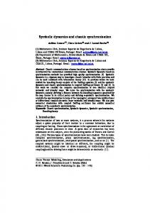
where R is the maximum and r the minimum value of the control parameter r t . t 0 is the latency time of the simulated time series and 2d is its duration. The latency time t 0 was allowed to jitter according to t 0 ⫹ ␶ , where ␶ was a uniformly distributed random number with zero mean and standard deviation ␴ ␶ . Figure 1 shows an example of the dependency of the mean control parameter 共averaged over all simulated trials兲 for the case where ␴ ␶ ⫽0, i.e., without any latency jitter. This function causes the logistic map to become nonstationary at t 0 ⫺d until t 0 ⫹d. We used a latency t 0 ⫽100 and as the duration of the transient regime 2d⫽30. Thus, the following figures should show some conspicuous behavior around t⫽100 where something is going on. The ensembles have been generated by choosing N initial conditions randomly and uniformly distributed in an interval 关 0,P 兴 , where P stands for the precision of the preparation of initial conditions. We ran simulations for N⫽30, which is a typical size of a single subject ERP ensemble, and for N ⫽1000 as a typical size of a grand ERP ensemble of all subjects collected together. The sample size was always L ⫽300. In the former we chose P⫽0.001 when ␴ ␰ ⫽0 and P⫽0.01 when ␴ ␰ ⫽0. In the latter, P⫽0.2 was chosen for all values of ␴ ␰ . For comparison between our symbolic dynamics technique and the traditional averaging approach of ERP, we calculated the ensemble averages of the simulated time series. The symbolic dynamics has been performed using the critical point x c ⫽0.5 of the logistic map as the dividing point

FIG. 1. Dependency of mean control parameter on time for an ensemble of logistic maps without noise ( ␴ ␰ ⫽0,␴ ␶ ⫽0) but with control parameter varying in the range R⫽4.0, r⫽3.0 关see Eq. 共27兲兴. The nonstationarity happens around t⫽100.

for a binary partition of the unit interval 关 0,1兴 ⫽A 0 艚A 1 , A 0 ⫽ 关 0,0.5 兴 , and A 1 ⫽]0.5,1] 关23兴. Furthermore, we created binary Bernoulli processes of the same ensemble size and the same number of samples in order to compare their entropies and word statistics with those given by the logistic map. We did three numerical experiments: 共a兲 with different maxima and minima of the control parameter but without any noise and any latency jitter, 共b兲 varying only the dispersion of the noise leaving the range of the control parameter and the latency invariant, and 共c兲 investigating the impact of latency jitter on ensemble averages and symbolic dynamics using a fixed range of the control parameter and no noise of the dynamics. In the first series of simulations, we chose the parameters of the model as N⫽30, L⫽300, P⫽0.001, R⫽4.0, ␴ ␰ ⫽ ␴ ␶ ⫽0, and r苸兵 3.0,3.8,3.85,3.95其 . The maximum R⫽4 corresponds to fully developed chaos, while for r⫽3.0 the map possesses an unstable fixed point at x * ⫽ 32 . At values between r ⬁ ⬇3.569 99 . . . 共the Feigenbaum attractor兲 and R ⫽4.0, the map shows very complicated behavior changing from chaotic bands to periodic windows and back to chaotic bands 共see, e.g., 关72兴兲. Figure 2 shows 共a兲 the averaged time series 具 x(t) 典 and 共b兲 the symbolic dynamics for the setting R⫽4.0, r⫽3.0, ␴ ␰ ⫽0, and ␴ ␶ ⫽0 with the change of the control parameter shown in Fig. 1. Black pixels denote the symbol ‘‘0’’ (x t 苸关 0,0.5 兴 ) and white pixels denote the symbol ‘‘1’’ (x t 苸兴 0.5,1]). Both Figs. 2共a兲 and 2共b兲 show clearly the change of the dynamics around t⫽100. At the very beginning, the systems behavior is transient while it settles at the chaotic attractor for R⫽4.0. In the averaged time series 共a兲 this nonstationarity is given by a fast, almost exponential increase of 具 x(t) 典 . In the symbolic dynamics, this transient behavior is indicated by a black vertical stripe, while the states evolve in A 0 ⫽ 关 0,0.5 兴 . At time t⫽85, the control parameter starts to depend on time, and the systems become nonstationary. This is indicated by the averages beginning to oscillate until the control parameter becomes constant at t ⫽115. In the symbolic dynamics, the transient regime is a

PRE 62


5525

FIG. 3. One-word statistics of the ensemble of logistic maps. Parameter settings: N⫽30, L⫽300, P⫽0.001, R⫽4.0, r⫽3.0, ␴ ␰ ⫽0, and ␴ ␶ ⫽0. Parameters are the same as Fig. 2.

FIG. 2. Time series from the logistic map 共a兲 Ensemble averages, 共b兲 symbolic dynamics. Black pixel, ‘‘0’’ (x t 苸关 0,0.5 兴 ); white pixel, ‘‘1’’ (x t 苸兴 0.5,1]). Parameter settings: N⫽30, L ⫽300, P⫽0.001, R⫽4.0, r⫽3.0, ␴ ␰ ⫽0, and ␴ ␶ ⫽0. The nonstationarity happens around t⫽100.

white vertical stripe, because the fixed point x * ⫽ 32 belongs to A 1 ⫽]0.5,1]. Figure 2 illustrates the differences of averaging time series and symbolic dynamics. One could expect that, by lowering the amplitude of the change in control parameter R⫺r, the jump of the averaged states will decrease and eventually be hidden by the chaotic dynamics. This will not happen in the symbolic dynamics unless the fixed point leaves the interval A 1 ⫽]0.5,1]. For the same example, Fig. 3 gives the statistics of words of length 1, i.e., the distribution of symbols over time. As in the visualization 关Fig. 2共b兲兴, the word statistics reveal clearly the phase transition from chaotic to periodic behavior at time t⫽85. The large white stripe in Fig. 2共b兲 corresponds to a degeneration of the word distribution where only the ‘‘word’’ ‘‘1’’ remains. Next, we shall tune the control parameter towards the fully developed chaotic regime. We present the ensemble averages of the time series generated by the logistic map for minimal control parameter settings r⫽3.8 共Fig. 4兲. It is ob-

vious that for diminishing distances R⫺r the phase transition at time t⫽85 becomes harder to recognize in the averages. But in contrast, Fig. 5 reveals that there is a change of the dynamics visible in the running cylinder entropies 关shown are Shannon entropies (q⫽1) for word length n⫽2, Fig. 5共a兲兴. Though also vanishing for r→R, the distinction remains significant by means of surrogate data 关Fig. 5共b兲兴, where M ⫽1000 surrogates have been generated. There are some further peaks of the significances at later times at 150 and 250. These could be explained by the fact that the logistic map is not fully chaotic for a parameter value r⫽3.8 and therefore significantly different from the Bernoulli process represented by the surrogates. Using the ␹ 2 -test to compare the data from the logistic map with those from the Bernoulli process fails for small ensembles because the ␹ 2 -test demands at least five occurrences of each word. Thus, we collected words within sliding windows according to Eq. 共26兲. This has been done for different word lengths in different windows. We present the results of the four-word statistics in sliding windows of length D⫽20 samples in Fig. 6.

FIG. 4. Ensemble averages of time series of the logistic map for minimal value of the control parameter: r⫽3.8. N⫽30, L⫽300, P⫽0.001, R⫽4.0, ␴ ␰ ⫽0, and ␴ ␶ ⫽0. Again, the nonstationarity happens around t⫽100.

5526


PRE 62

FIG. 6. Significance 关 ⫺log10(p error) 兴 of the ␹ 2 -test between word statistics of symbolic dynamics of the logistic map and Bernoulli process in sliding windows. r⫽3.8, word length: n⫽4, sliding window length D⫽20, N⫽30, L⫽300, P⫽0.001, R⫽4.0, ␴ ␰ ⫽0, and ␴ ␶ ⫽0.

FIG. 5. Running normalized Shannon cylinder entropies 关Eqs. 共22兲 and 共23兲兴共a兲 and their significances 共b兲 from M ⫽1000 surrogates 关Eq. 共25兲兴 of the symbolic dynamics in comparison to a Bernoulli process. Solid, logistic map; dashed, Bernoulli process. Word length: n⫽2, q⫽1.0. 共a兲,共b兲 r⫽3.8, N⫽30, L⫽300, P⫽0.001, R⫽4.0, ␴ ␰ ⫽0, and ␴ ␶ ⫽0. Note the nonstationarity around t ⫽100.

Finally, we show the Shannon entropies obtained from these word statistics in a sliding window. Figure 7 shows the result for r⫽3.8. In contrast to the running cylinder entropies that drop in the periodic regime of the dynamics, the entropies of the sliding window cylinders increase at the beginning and at the end of the phase transition while they drop in between. This increase in entropy is explained by the fact that the dynamical behavior becomes richer when the sliding window crosses the onset of the phase transition: On the left the dynamics remain chaotic but on the right side of the window the dynamics become periodic. Between both peaks, these entropies drop when the sliding window is entirely contained within the transient regime of the dynamics. This is the case in the simulation because the sliding window length D⫽20 is smaller than the duration 2d⫽30 of the nonstationarity. The pattern shown in Fig. 7 should be the same even if there is an uncertainty in latency. This will be addressed in Sec. IV C.

changes in control parameter and, in the presence of noise, it is also sensitive to the noise level. In the following, we increase the standard deviation of noise according to ␴ ␰ 苸兵 0.0005,0.001,0.002,0.0021,0.0022,0.002 21其 . Figure 8 shows the fourth-order Shannon entropies for the simulations with 共a兲 ␴ ␰ ⫽0.0, 共b兲 ␴ ␰ ⫽0.001, 共c兲 ␴ ␰ ⫽0.002, and 共d兲 ␴ ␰ ⫽0.002 21, while Fig. 9 presents the ␹ 2 -significances of the four-word statistics between logistic maps for timedependent and fixed values of the control parameters of the same ensemble size. The parameter of the control condition has been fixed to R⫽r⫽3.569 99. While dynamical noise destroys any distinction in the averaged time series at the critical value r ⬁ , the symbolic dynamics remains a reliable detector of phase transitions even in the presence of noise. The only impact of noise on the running entropies is that the differences of the dynamics before and after the nonstationary regime 关oscillations at time t⫽150, Fig. 8共a兲兴 are smeared out. C. Changing latency jitter

Finally, we study the impact of latency jitter on symbolic dynamics of simulated data and measures of complexity. We created 30 time series per condition for the control parameter

B. Changing noise level

Next, we study simulations where N⫽1000 initial conditions in the range 关0,0.2兴 have been prepared. We chose R ⫽3.569 99, the parameter value near the Feigenbaum attractor, and r⫽3.4 in the periodic regime again. At the Feigenbaum attractor, the logistic map is very sensitive to small

FIG. 7. Shannon entropies (q⫽1) of the word statistics of symbolic dynamics of the logistic map in sliding windows. r⫽3.8, word length: n⫽4, sliding window length D⫽20, N⫽30, L ⫽300, P⫽0.001, R⫽4.0, ␴ ␰ ⫽0, and ␴ ␶ ⫽0.

PRE 62


5527

FIG. 8. Running Shannon cylinder entropies of the symbolic dynamics of the noisy logistic map for different additive noise strength in comparison to a Bernoulli process. Solid, logistic map; dashed, Bernoulli process. Word length: n⫽4, q⫽1.0. 共a兲 ␴ ␰ ⫽0.0, 共b兲 ␴ ␰ ⫽0.001, 共c兲 ␴ ␰ ⫽0.002, 共d兲 ␴ ␰ ⫽0.002 21. 共a兲–共d兲 N⫽1000, L⫽300, P⫽0.02, R⫽3.569 99, r⫽3.4, and ␴ ␶ ⫽0.

FIG. 9. Significance 关 ⫺log10(p error) 兴 of the ␹ 2 test between word statistics of symbolic dynamics of the noisy logistic map for different additive noise strength against the undisturbed logistic map with constant control parameter r⫽R⫽3.569 99. Word length: n⫽4. 共a兲 ␴ ␰ ⫽0.0, 共b兲 ␴ ␰ ⫽0.001, 共c兲 ␴ ␰ ⫽0.002, 共d兲 ␴ ␰ ⫽0.002 21. 共a兲–共d兲 N⫽1000, L⫽300, P⫽0.02, R⫽3.569 99, r⫽3.4, ␴ ␶ ⫽0.

5528


PRE 62

FIG. 10. Shannon entropies (q⫽1) of the four-word statistics of the symbolic dynamics of the logistic map with varying latency jitter in sliding windows. 共a兲 ␴ ␶ ⫽0, 共b兲 ␴ ␶ ⫽2, 共c兲 ␴ ␶ ⫽6, 共d兲 ␴ ␶ ⫽10. 共a兲–共d兲 Sliding window length D⫽20, R⫽4.0, r⫽3.8, N⫽30, L⫽300, P⫽0.001, R⫽4.0, and ␴ ␰ ⫽0.

values R⫽4.0, r⫽3.8, and increased the standard deviation of latency jitter according to ␴ ␶ 苸兵 0,1, . . . ,15,20其 . First, we show the Shannon entropies of four-words collected in a sliding window of length D⫽20 共Fig. 10兲 for 共a兲 ␴ ␶ ⫽0, 共b兲 ␴ ␶ ⫽2, 共c兲 ␴ ␶ ⫽6, and 共d兲 ␴ ␶ ⫽10, whereas Fig. 11 presents the ␹ 2 significances of these four-word statistics between the logistic map and a Bernoulli process for 共a兲 ␴ ␶ ⫽5 and 共b兲 ␴ ␶ ⫽10. The phase transition of the dynamics remains significant for small as well as for large dispersions of latency time even if there is no difference visible in the ensemble averages. For a latency jitter of ␴ ␶ ⫽20 we obtained significance better than the 10⫺5 confidence level. The spurious peaks at times t⫽50 and about t⫽260 can be neglected by choosing a significance threshold smaller than 10⫺5 . Our numerical experiments with a noisy logistic map and four freely controlled parameters — r,R,␴ ␰ , ␴ ␶ — mimicking some properties of ERP data, such as different experimental conditions, spontaneous brain activity, and latency jitter, have shown that symbolic dynamics andmeasure of complexity are able to distinguish transient regimes of behavior from stationary dynamics much better than averages of time series can do. Also symbolic dynamics provide many parameters such as different partitions, word lengths, sliding windows, and q values of Reńyi entropies. These parameters must be appropriately chosen in order to obtain the best result of data analysis. We varied these parameters quite arbitrarily to illustrate the dependence of results from these choices. For example, Figs. 5 and 8 demonstrate the impact of the word length on running entropies and it seems to be the case that longer words will provide better

FIG. 11. Significance 关 ⫺log10(p error) 兴 of the ␹ 2 -test between word statistics of the symbolic dynamics of the logistic map with varying latency jitter and Bernoulli process in sliding windows. 共a兲 ␴ ␶ ⫽5, 共b兲 ␴ ␶ ⫽10. 共a兲,共b兲 Sliding window length D⫽20, R⫽4.0, r⫽3.8, N⫽30, L⫽300, P⫽0.001, R⫽4.0, and ␴ ␰ ⫽0.

PRE 62


5529

FIG. 12. Single subject voltage averages for the VERB condition 共solid lines兲 compared to the CONTROL-VERB condition 共dotted兲. Lower panels: potential 共␮V兲 against time 共s兲, t⫽0: stimulus onset time. Upper panels: t-test error probabilities 共logarithmic scale兲. The ungrammaticality effect, P600 共positive peak after 600 ms兲, is marked by arrows. For channel labeling see text.

results than shorter words. But for strong noise or small ensemble sizes the opposite holds, as we saw for data obtained from different ERP experiments. However, we have shown that nonstationary dynamics can be detected from ensembles of coarse-grained time series even if there are very small changes in the control parameters and the system is sensitive against changes in initial conditions as well as changes in control parameter. This applies also in the presence of dynamical 共and not only observational兲 noise. In addition, by using sliding windows, our method is able to track uncertainty about the time when changes of the control parameters happen. V. ANALYSIS OF EXPERIMENTAL DATA A. Setup

In this section we shall compare the traditional ERP averaging technique with our methods based on symbolic dynamics for ERP data acquired in the Potsdam Language Processing Laboratory. We performed a language-processing experiment in which subjects were seated in front of a monitor for stimulus presentation. They were wired with the EEG amplifier device by a 32-channel electrocap. The EEG data have been recorded in 25 channels according to the international 10-20 system at a sampling rate of 250 Hz with the ScanAmps/NeuroScan recording system against reference at the left mastoid bone and grounded by the electrode Fpz.

Four channels were used for measuring EOG artifacts. ERP data have been digitally band-pass-filtered at 0.2–29 Hz after manual artifact rejection. 150 sentences, 30 sentences for each condition, organized in five blocks, were visually presented to subjects word by word but in randomized order with a presentation time and interstimulus interval of 400 ms. At the end of each sentence, subjects had to indicate whether or not a target word had occurred in the preceding sentence. The experiment was performed in two runs, the first without and the second including distractor sentences in order to mislead subjects about the purpose of the study. We report here the data analysis of 16 subjects 共15 female兲 aged 19–25, mean age 21.78 years. The subjects were volunteers, students of the University of Potsdam, native speakers of German but not familiar with the purpose of the study. The sentences presented to the subjects were initially ambiguous interrogative sentences. The point of disambiguation 共i.e., where the meaning becomes clear兲 was either at the verb or at the second article. For details, see Appendix A 2 or 关73兴; an introduction into language-related brain activity can be found in 关48,4,49兴. B. Single subject analysis

First, we discuss the results of traditional averaging analysis and symbolic dynamics obtained from the data of a single subject. Digitally band pass filtering, epoching, averaging,

5530


PRE 62

FIG. 13. Single subject symbolic dynamics of the CONTROL-VERB condition. Statically encoded after transform to a uniform distribution. Black pixel, ‘‘0’’ (r t 苸关 0,0.5 兴 ); white pixel, ‘‘1’’ (r t 苸兴 0.5,1]).

FIG. 14. Single subject symbolic dynamics of the VERB condition. Statically encoded after transform to a uniform distribution. Black pixel, ‘‘0’’ (r t 苸关 0,0.5 兴 ); white pixel, ‘‘1’’ (r t 苸兴 0.5,1]).

PRE 62


5531

FIG. 15. Running Shannon entropies for the VERB condition 共solid lines兲 compared to the CONTROL-VERB condition 共dotted兲 for single subject data. Panels: normalized Shannon entropy of one word (n⫽1;q⫽1.0) in bit/ sample against time 共s兲, t⫽0: stimulus onset time.

FIG. 16. Significance of the Shannon entropy for the CONTROLVERB condition of single subject data by means of M ⫽100 surrogates simulating a Bernoulli process. Panels: Significance measure S D 共unit ␴兲 against time 共s兲, t⫽0: stimulus onset time.

5532


PRE 62

FIG. 17. Significance of the Shannon entropy for the VERB condition of single subject data by means of M ⫽100 surrogates simulating a Bernoulli process. Panels: Significance measure S D 共unit ␴兲 against time 共s兲, t⫽0: stimulus onset time.

FIG. 18. Significance 关 ⫺log10(p error) 兴 of the ␹ 2 -test between one-word statistics of the VERB condition against the CONTROL-VERB condition of single subject data in sliding windows of length D⫽20 ms.

PRE 62


5533

FIG. 19. Voltage grand averages for the VERB condition 共solid lines兲 compared to the CONTROLVERB condition 共dotted兲. Lower panels: potential 共␮V兲 against time 共s兲, t⫽0: stimulus onset time. Upper panels: t-test error probabilities 共logarithmic scale兲. The ungrammaticality effect, P600 共positive peak after 600 ms兲, is marked by arrows.

and visualization of ERP data have been performed using the EEP 共event related potential evaluation package兲 software developed by the Max Planck Institute for Cognitive Neuroscience 关74兴. We present first the voltage averages of the VERB condition in comparison to its CONTROL-VERB condition. Figure 12 shows a 3⫻3-channel subarray consisting of the electrodes BL, Fz, and BR in the first row; WL, Cz, and WR in the second row; and P3, Pz, and P4 in the last. The labels Fz, Cz, P3, Pz, and P4 are due to the naming convention of the international 10-20 system, where the first symbol denotes the cortical lobes 共F, frontal; T, temporal; O, occipital; P, parietal兲 or the vertex 共C, central兲. The second symbol is either ‘‘z’’ 共midline兲 or a number. Odd numbers correspond to the left hemisphere and even numbers to the right. The labels BL, BR and WL, WR denote language-specific cortical areas 共B, Broca’s; W, Wernicke’s areas兲 at the left 共L兲 or right 共R兲 hemisphere. In the electrode array shown by Fig. 12, two diagrams are assigned to each channel: At the bottom, the time course of the averaged voltages is shown 关86兴. The solid line represents the experimental condition 共VERB兲 while the dotted line indicates the signal of the control condition 共CONTROL-VERB兲. The latter has been gained by averaging over 21 trial epochs, the former by averaging over 25 trials for the subject chosen here. At the top we show the confidence levels of a running t-test performed pointwise at each sampling point between both conditions. Significant time regions are indicated by error probabilities above the ␣ ⫽0.01(99%) threshold. Obviously, the VERB condition differs significantly from the CONTROL-VERB condition by a huge positive voltage deflection about 600 ms after verb pre-

sentation. This is known as the P600 ERP component 共positivity after 600 ms兲 and has been related to reanalysis processes achieved by the human language-processing system dealing with local ungrammaticalities 关48兴. Next, we apply our newly developed techniques based on symbolic dynamics on these data. Figures 13 and 14 present the corresponding single subject symbolic dynamics of the CONTROL-VERB and the VERB condition, respectively. According to our discussion in Sec. III D, a partition of the state space or a corresponding partition of the range of the observables that are generated by the dynamical system is needed in order to obtain a symbolic dynamics. Either one encodes the values of time series into symbols by a certain binning 共this method is called static encoding兲, or one encodes differences between succeeding samples as estimators of local slopes 共this is called dynamic encoding兲关25兴. We decided to use static encoding after we had transformed each voltage epoch to a uniformly distributed time series by a ranking procedure. Ranking, an additional step of preprocessing, has several advantages in signal analysis because it corresponds to a nonlinear but smooth and invertible mapping of data x t due to their distribution function F. Relative rank numbers r t ⫽R t /L depending on time are then obtained by the transform r t ⫽F(x t ). Since the map F is a homeomorphism, ranking does not disturb the topological properties of state space and thus leaves basic quantities such as Lyapunov exponents or Kolmogorov entropies invariant 关75兴. A numerical problem linked to ranking methods arises when some values occur several times in the data set. Using sorting algorithms leads to consecutive rank numbers for the same value of

5534


PRE 62

FIG. 20. Running normalized Reńyi entropies for the VERB condition 共solid lines兲 compared to the CONTROL-VERB condition 共dotted兲 of the grand ensemble. Panels: Reńyi entropy of one word (n⫽1;q⫽10.0) in bit/sample against time 共s兲, t⫽0: stimulus onset time. The ungrammaticality effect, P600 共positive peak after 600 ms兲, is marked by arrows. Additionally, the attention shift indicator 共N100兲 is marked by arrows.

data. Pompe recommends solving this problem of ‘‘tied ranks’’ by replacing the measured values x t by some disturbed values x t ⫹a i before doing the ranking, where 0⭐a i ⭐a i⫹1 ⭐1 共关75兴, p. 85兲. We used white noise of different variances added to the voltages to tackle this problem, but we found no significant differences compared to tied ranks which have been admitted. Performing a binary static encoding after the ranking procedure according to the median 关 F(x med)⫽0.5兴 of each epoch separately as the decision point yields a symbolic sequence containing the same number of ‘‘0’’ (r t ⭐0.5) and ‘‘1’’ (r t ⬎0.5). Thus, ranking maximizes the entropy of each sequence. However, the visualized data in Figs. 13 and 14 show distinct patterns of more or less vertical stripes. The P600 ERP component is again clearly visible as a wide white band occurring mainly at 600 ms in the channels BL, Fz, and Cz 共Fig. 14兲. The static encoding strategy provides, therefore, an interface between ERP voltage averages and symbolic dynamics techniques that allows for comparisons between both methods. Simple static encodings by assigning, e.g., ‘‘0’’ to negative and ‘‘1’’ to positive voltage deflections have already been proposed in the early 1970s by Lehmann 关76兴. Counting symbol occurrences from all epochs at a certain point in time 关in our terms one-word statistics, see Eq. 共21兲兴 is well known as polarity histograms in the ERP literature 关41兴. However, simple static encoding of voltages requires some baseline correction.

Next, we are going to quantify the patterns visible in Figs. 13 and 14. Our concepts of running cylinder entropies 关Eqs. 共22兲–共24兲兴 are appropriate tools for quantifying vertical stripes because every vertical band of the symbolic dynamics can be considered as a family of cylinder sets. Figure 15 presents the Shannon entropies calculated from these running cylinders of length n⫽1 for the VERB condition 共solid line兲 and the CONTROL-VERB condition 共dotted line兲, respectively. In order to determine whether these changes in entropy are significant or not, we computed the average Shannon entropies from an ensemble of M ⫽100 surrogate data according to Eq. 共25兲 generated by shuffling the symbols of each epoch in time. Figures 16 and 17 show these results for the CONTROL-VERB condition and the VERB condition, respectively. Figures 15 and 17 demonstrate a highly significant entropy drop in the VERB condition around 600 ms after stimulus presentation, whereas the entropy curve remains flat in the CONTROL-VERB condition in this time domain. There are also some significant events in both conditions in channels BL, BR, and WR at time 100–200 ms as well as in channels P3 and P4 in the 300-ms time period shown in Figs. 15, 16, and 17. The early event is the N100 attention shift mentioned in Sec. II. The electrodes P3 and P4 are situated near the primary visual cortex, so they indicate optical information processing at time 300 ms. Cylinder measures are the appropriate tool for studying patterns such as vertical stripes. But as mentioned above, the

PRE 62


5535

FIG. 21. Significance 关 ⫺log10(p error) 兴 of the ␹ 2 test between one-word statistics of the VERB condition against the CONTROL-VERB condition of the grand ensemble in sliding windows of length D⫽20 ms. Again, P600 and N100 are marked by arrows.

symbolic dynamics of ERP are meandering bands rather than vertical stripes due to the latency jitter. Thus, we need some measures of ‘‘stripiness.’’ These are provided by word statistics collected in sliding windows and their corresponding entropies given by Eq. 共26兲. For single subject investigations, collecting words in sliding windows is also necessary in order to fulfill the requirements of the ␹ 2 -test, where at least five events should be counted into one bin. Finally, Fig. 18 shows the result of the ␹ 2 -test comparing the VERB condition against the control condition by their one-word statistics in a sliding window of 20 ms. The level of confidence for the P600 at electrode Fz is better than 10⫺8 . C. Grand ensemble analysis

At the end of this study we compare the results of the grand average analysis and the grand ensemble analysis of the symbolic dynamics gained from all 16 subjects together. Figure 19 gives the voltage grand averages of the VERB condition 共solid lines兲 and the CONTROL-VERB condition 共dotted lines兲. Only the P600 ERP component appears to be highly significant by means of the running t test. Figure 20 presents the Reńyi entropy comparison for word length n⫽1 and q⫽10.0. The VERB condition is plotted solid and the CONTROL-VERB condition dotted, again. This entropy plot shows not only the P600 component but also an early entropy drop symmetrically distributed at the frontal sites BL, Fz, Cz, and BR. This is the N100 attention

shift ERP marker we mentioned before. In contrast to the voltage averages, this event becomes significant in the symbolic dynamics between both conditions. Figure 21 shows the corresponding ␹ 2 -error probabilities of one-word statistics collected in 20-ms sliding windows. It comes out that both the P600 as well as the very early entropy drop are significantly better than the 10⫺8 confidence level. So far we have been only interested in the dynamics at single sites. The behavior of ERP over the whole scalp can be shown using brain-mapping techniques. We shall present brain maps of Reńyi entropy (n⫽1,q⫽10) differences between the VERB and the CONTROL-VERB condition at single instances of time and their corresponding significance maps obtained by the ␹ 2 -test of one-word statistics collected in 20-ms sliding windows. Figure 22共a兲 shows the P600 at time 616 ms as a left frontal distributed blacking 共the VERB condition has been subtracted from the CONTROL-VERB condition; hence, the entropy drop is shown black兲. Figure 22共b兲 shows the significance map of the windowed ␹ 2 test. Figure 23 gives a legend of the brain map. Let us take a look at the other experimental conditions that have been tested in the language-processing ERP experiment. Figure 24 shows the voltage grand averages for the ARTICLE 共solid line兲 against the CONTROL-ARTICLE 共dotted兲 condition in a 3⫻3 array. By means of the running t-test 共upper panel兲 there are no later events that turn out to be

5536


PRE 62

FIG. 23. Map legend of the electrode array. VI. DISCUSSION

FIG. 22. 共a兲 Reńyi entropy difference map of the VERB condition subtracted from CONTROL-VERB condition of the P600 ERP of the grand ensemble (n⫽1;q⫽10.0). 共b兲 Significance map 关 ⫺log10(p error) 兴 of the windowed ␹ 2 -test of one-word statistics in a sliding 20-ms window.

significant at p⬍0.01. Both curves are close together at almost all times. Note, there is a very late effect at 800 ms in channels Fz and Cz where the voltage averages of the ARTICLE condition vanish. In the traditional ERP terminology, there is no ERP component, because the voltage average curve does not possess a peak in this time range. We present brain maps of Reńyi entropy differences (n ⫽1,q⫽10) of the ARTICLE and the CONTROL-ARTICLE condition and their corresponding significance map at two instances of time. Figure 25 shows these maps at time 210 ms after stimulus onset. Figure 25共a兲 reveals an increase in entropy at posterior sites WL and WR represented by white areas, which becomes more significant at WL 关Fig. 25共b兲兴. The late effect is given at time 830 ms in Figs. 26共a兲 and 26共b兲. The vanishing voltage average corresponds to an entropy increase distributed at the left anterior areas 共electrodes F3 and BL兲. Thus, we have proven that there is more structure in ERP data than could be discovered by averaging voltages. Our techniques resting on symbolic dynamics and measures of complexity provide access to these hidden structures in the data.

In this study we have criticized the prerequisites of the traditional ERP averaging technique based on stationary and ergodicity properties and intertrial independence of background EEG as well as on intertrial invariance of the assumed ERP signal. Due to these unrealistic assumptions, we have proposed an alternative approach of ERP time series analysis resting on statistical mechanics of dynamical systems and mainly on symbolic dynamics and measures of complexity. We have validated this ansatz by simulations of transient noisy nonlinear dynamics and applied it to real ERP data given by a language-processing ERP experiment. Our method reproduces well-known ERP components such as the P600 of syntactic reanalysis as highly significant entropy drops. We tested data for significance using either the method of surrogates in order to distinguish patterns in the symbolic dynamics indicated by changes in entropies from Bernoulli processes, or by means of a nonparametric ␹ 2 test. Thus, we should not assume that data were Gaussian distributed or had stationary variances as is necessary for applying t tests or analyses of variance. Employing a ␹ 2 test requires statistical independence of trial epochs, of course. But this can be approximately fulfilled by the experimental design, e.g., by randomization of stimuli concerning experimental conditions or by using distractor sentences. We not only regained the well-known ERP component P600, but we also found a very early entropy drop 共corresponding to a modulation of the attention shift N100 ERP兲 that is highly significant in our analysis but not in the comparison of mean voltage differences. Thus, our method is more sensitive to qualitative changes in the ongoing EEG than the averaging technique. While classical ERP components are reflected by drops in entropy of the experimental condition relative to the control condition, the second part of the study shows increasing relative entropies that also become significant. There are no counterparts to these events in the traditional ERP paradigm at all. These findings together with the theoretical basis of our method suggest viewing ERP components as information sources of a given entropy rate 关62兴 rather than a particular signal hidden by some noisy background that must be extracted from the data. Since symbols and words formed by strings of symbols of a symbolic dynamics correspond to regions of the phase space, periods of time of low cylinder entropy can be seen as bottlenecks in the state space in analogy to channeling in the case of intermittency. On the other hand, periods of time of increased cylinder entropy are periods where a greater volume of phase space is available to the dynamics. This interpretation agrees further with the results reported in 关22兴 concerning the dynamics of pointwise di-

PRE 62


5537

FIG. 24. Voltage grand averages for the ARTICLE condition 共solid lines兲 compared to the CONTROL-ARTICLE condition 共dotted兲. Lower panels: potential 共␮V兲 against time 共s兲, t⫽0: stimulus onset time. Upper panels: t-test error probabilities 共logarithmic scale兲.

mensions. Molna´r et al. showed that the P300 ERP component found in the oddball experiment 共see the Introduction兲 is reflected by a drop in pointwise correlation dimension. Our approach has the advantage that it requires only counting of words and computing entropies and significances. It neither demands the application of embedding techniques nor employs least-square fits to almost linear scaling regions. So far, we have shown that methods of symbolic dynamics and measures of complexity are able to capture the wellknown ERP components. Additionally, our newly developed techniques reveal more structure hidden in the data. However, there remain open questions. Using a static symbolic encoding of data after performing a ranking procedure enables us to compare the results directly with voltage averages provided by the traditional technique. On the other hand, dynamical or mixed strategies of coarse graining may provide better insights into neural information processing since the first derivative of evoked potentials seems to be related to the firing probability of neurons 关关52兴, p. 40兴. However, such results might be hard to interpret without an interface to voltage averages. One central issue is the interpretation of ERP in terms of brain dynamics. The traditional averaging technique assumes the ERP’s to be deterministic signals generated by the brain as responses to certain stimuli or cognitive events. Data analysis is thus the job of improving the signal-to-noise ratio 关38兴. Alternatively, we can view ERP’s as indicators of reorganization in the ongoing spontaneous EEG activity. By using methods of spectral analysis, one can show that the distributions of phase spectral values of ERP epochs are different between experimental conditions, while distributions of amplitudes are not 关38兴. Also symbolic dynamics neglects some information about amplitudes but it restores information about timing. Hence, the question of synchronization and phase locking of neuronal oscillators arises in the con-

text of ERP studies 关52,77–81兴. A further issue is the role of spatiotemporal correlations of ERP. These could be investigated using the notions of conditional entropy and mutual information in the framework of symbolic dynamics 关62,75兴.

ACKNOWLEDGMENTS

We would like to thank Ralf Engbert, Gu¨nter Troll, Thomas Liebscher, and Kelly Sloan for stimulating and helpful discussions and for a critical reading of the manuscript. Wolfgang Jansen’s support concerning numerical problems is gratefully acknowledged. We thank Sandra Neumayer and Saskia Kohnen for their work in the laboratory as well as Bryan Jurish for fixing all computer problems. This work has been supported by the Deutsche Forschungsgemeinschaft within the scientists group on conflicting rules in cognitive systems.

APPENDIX 1. Proof of the partitioning lemma

Assume we have a 共time discrete兲 dynamical system (X,⌽ r ) together with an observable h:X→R that maps states onto real numbers. Let h(X)⫽H傺R be the image of X under the action of h. Now, we choose a partition S i , i ⫽1,2, . . . ,I of H and determine the preimages of the sets S i in X: A i ⫽h ⫺1 (S i ). According to a basic theorem of set theory for any map f :X→Y holds, f ⫺1 共 A艚B 兲 ⫽ f ⫺1 共 A 兲艚 f ⫺1 共 B 兲 ,

共A1兲

f ⫺1 共 A艛B 兲 ⫽ f ⫺1 共 A 兲艛 ⫺1 共 B 兲

共A2兲

5538


PRE 62

FIG. 25. 共a兲 Reńyi entropy difference map of the ARTICLE condition subtracted from CONTROL-ARTICLE condition of the left early entropy rise of the grand ensemble (n⫽1;q⫽10.0). 共b兲 Significance map 关 ⫺log10(p error) 兴 of the windowed ␹ 2 -test of one-word statistics in a sliding 20-ms window.

FIG. 26. 共a兲 Reńyi entropy difference map of the ARTICLE condition subtracted from CONTROL-ARTICLE condition of the late entropy rise of the grand ensemble (n⫽1;q⫽10.0). 共b兲 Significance map 关 ⫺log10(p error) 兴 of the windowed ␹ 2 -test of one-word statistics in a sliding 20-ms window.

for all A,B傺Y . Hence we compute first A i 艚A j A i 艚A j ⫽h ⫺1 (S i )艚h ⫺1 (S j )⫽h ⫺1 (S i 艚S j )⫽⭋, if i⫽ j. And secI I I S i )⫽ 艛 i⫽1 h ⫺1 (S i )⫽ 艛 i⫽1 Ai ond h ⫺1 (H)⫽h ⫺1 ( 艛 i⫽1 ⫽X.

presented to the subjects were initially ambiguous interrogative sentences. The point of disambiguation was either at the verb 共VERB condition兲 or at the second article 共ARTICLE condition兲. The control sentences were not ambiguous at these points. Table I shows examples of the German sentences, an English paraphrase, and the correct English translation. The critical words where ERP measurement took place are printed in italics. Interrogative sentences in German are usually expected to be of subject-verb-object order 共examples: CONTROL-VERB, CONTROL-ARTICLE兲. But object-verb-subject order is also possible 共examples: VERB and ARTICLE兲. The first two words in the sentences, ‘‘welche Frau,’’ are ambiguous with respect to nominative or accusative case and are always the same. Subjects expect the sentences to be of the frequent subject-verb-object structure. There are two ways for disambiguating such sentences: either by the number feature, i.e.,

2. The language-processing experiment

The ERP experiment was performed using 30 structurally equivalent sentences for each condition and five conditions total. We report here the results of two experimental conditions: VERB and ARTICLE against their corresponding control conditions CONTROL-VERB and CONTROL-ARTICLE. As mentioned before, the sentences were presented word by word showing the stimuli for 400 ms followed by a break of 400 ms, too. The sampling of ERP epochs started 200 ms before the critical word occurred and finished 1000 ms after. Thus, at time t⫽0 ms the critical words appeared. The sentences


PRE 62

5539

TABLE I. Example sentences of the language-processing ERP experiment. Critical words 共where ERP measurements happen兲 are printed in italics. Condition

Example

Paraphrase

Translation

welche Frau sahen die Ma¨nner?

which woman 共accusative singular兲 saw 共plural兲 the men 共nominative plural兲?

which men saw the woman?

CONTROL-VERB

welche Frau sah den Mann?

which woman 共nominative singular兲 saw 共singular兲 the men 共accusative singular兲?

which woman saw the man?

ARTICLE

welche Frau sah der Mann?

which woman 共accusative singular兲 saw 共singular兲 the man 共nominative singular兲?

which man saw the woman?

CONTROL-ARTICLE

welche Frau sah den Mann?

which woman 共nominative singular兲 saw 共singular兲 the man 共accusative singular兲?

which woman saw the man?

VERB

subject-noun and verb must agree in number 共singular or plural兲, or by the case feature, i.e., the subject-noun has the nominative case, whereas the object-noun bears the accusative case. In the VERB condition the disambiguating information comes at the verb that does not agree with the subject-noun in number: the subject noun ‘‘Frau’’ is singular, the verb ‘‘sahen’’ is plural. The sentence seems to be ungrammatical at that point and a reanalysis of the structure built so far must take place. The P600 ERP component indicates this revision

of structure and meaning caused by the violation of expectation. In the ARTICLE condition the additional information is provided by the article ‘‘der’’ that is nominative case marked 共an accusative case marked article would be ‘‘den’’兲. As in the VERB condition, the sentence must be reanalyzed, but there is no significant event in voltage ERP averages. We show that in the ARTICLE condition the entropy increases compared with the CONTROL-ARTICLE condition 共for further reading, see 关73兴兲.

关1兴 Essentials of Neural Science and Behavior, edited by E. R. Kandel, J. H. Schwartz, and T. M. Jessel 共Appleton & Lange, East Norwalk, CT, 1995兲. 关2兴 D. Johnston and S. M.-S. Wu, Foundations of Cellular Neurophysiology 共MIT Press, Cambridge, MA, 1997兲, 3rd printing. 关3兴 P. L. Nunez, Electric Fields of the Brain 共Oxford University Press, New York, 1981兲. 关4兴 M. Rugg, in Cognitive Neuroscience, edited by M. Kutas and A. Dale 共Psychology Press, Hove East Sussex, 1997兲, pp. 197–242. 关5兴 H. Haken, Principles of Brain Functioning, Springer Series in Synergetics Vol. 67 共Springer, Berlin, 1996兲. 关6兴 J. A. S. Kelso, Dynamic Patterns. The Self-Organization of Brain and Behavior 共MIT Press, Cambridge, MA, 1999兲, 3rd printing. 关7兴 A. Babloyantz, J. M. Salazar, and C. Nicolis, Phys. Lett. 111A, 152 共1985兲. 关8兴 P. E. Rapp, I. D. Zimmerman, A. M. Albano, G. C. deGuzman, N. N. Greenbaun, and T. R. Bashore, in Nonlinear Oscillations in Biology and Chemistry, edited by H. G. Othmer, Lecture Notes in Biomathematics Vol. 66 共Springer, Berlin, 1986兲, pp. 175–205. 关9兴 A. M. Albano, N. B. Abraham, G. C. Guzman, M. F. H. Tar-

roja, D. K. Bandy, R. S. Gioggia, P. E. Rapp, I. D. Zimmerman, N. N. Greenbaum, and T. R. Bashore, in Mayer-Kress 关82兴, pp. 231–240. A. Babloyantz, in Mayer-Kress 关82兴, pp. 241–245. S. P. Layne, G. Mayer-Kress, and J. Holzfuss, in Mayer-Kress 关82兴, pp. 246–256. P. E. Rapp, T. E. Bashore, J. M. Martinerie, A. M. Albano, I. D. Zimmerman, and A. I. Mees, Brain Topogr. 2, 99 共1989兲. D. Gallez and A. Babloyantz, Biol. Cybern. 64, 381 共1991兲. W. Lutzenberger, T. Elbert, N. Birbaumer, W. J. Ray, and H. Schupp, Brain Topogr. 5, 27 共1992兲. W. S. Pritchard and D. W. Duke, Psychophysiology 29, 182 共1992兲. E. T. Bullmore, M. J. Brammer, P. Bourlon, G. Alarcon, C. E. Polkey, R. Elwes, and C. D. Binnie, Electroencephalogr. Clin. Neurophysiol. 91, 337 共1994兲. T. Elbert, W. J. Ray, Z. J. Kowalik, J. E. Skinner, K. E. Graf, and N. Birbaumer, Physiol. Rev. 74, 1 共1994兲. C. Besthorn, H. Sattel, C. Geiger-Kabisch, R. Zerfass, and H. Fo¨rstl, Electroencephalogr. Clin. Neurophysiol. 95, 84 共1995兲. A. R. Osborne and A. Provenzale, Physica D 35, 357 共1989兲. P. E. Rapp, A. M. Albano, T. I. Schmah, and L. A. Farwell, Phys. Rev. E 47, 2289 共1993兲.

关10兴关11兴关12兴关13兴关14兴关15兴关16兴

关17兴关18兴关19兴关20兴

5540


关21兴 J. Theiler, S. Eubank, A. Longtin, B. Galdrikian, and J. D. Farmer, Physica D 58, 77 共1992兲. 关22兴 M. Molna´r, J. E. Skinner, V. Cse´pe, I. Winkler, and G. Karmos, Electroencephalogr. Clin. Neurophysiol. 95, 118 共1995兲. 关23兴 B.-L. Hao, Physica D 51, 161 共1991兲. 关24兴 X. Z. Tang and E. R. Tracy, Chaos 8, 688 共1998兲. 关25兴 R. Wackerbauer, A. Witt, H. Atmanspacher, J. Kurths, and H. Scheingraber, Chaos, Solitons and Fractals 4, 133 共1994兲. 关26兴 J. S. Shiner, M. Davison, and P. T. Landsberg, Phys. Rev. E 59, 1459 共1999兲. 关27兴 J. Kurths, A. Voss, A. Witt, P. Saparin, H. J. Kleiner, and N. Wessel, Chaos 5, 88 共1995兲. 关28兴 M. Schiek, F. R. Drepper, R. Engbert, H. H. Abel, and K. Suder, in Kantz et al. 关83兴, pp. 191–213. 关29兴 C. Scheffczyk, A. Zaikin, M. Rosenblum, R. Engbert, R. Krampe, and J. Kurths, Int. J. Bifurcation Chaos Appl. Sci. Eng. 7, 1441 共1997兲. 关30兴 R. Engbert, C. Scheffczyk, R. T. Krampe, M. Rosenblum, J. Kurths, and R. Kliegl, Phys. Rev. E 56, 5823 共1997兲. 关31兴 P. Tass, J. Kurths, M. Rosenblum, G. Guasti, and H. Hefter, Phys. Rev. E 54, R2224 共1996兲. 关32兴 P. I. Saparin, W. Gowin, J. Kurths, and D. Felsenberg, Phys. Rev. E 58, 6449 共1998兲. 关33兴 P. E. Rapp, I. D. Zimmerman, E. P. Vining, N. Cohen, A. M. Albano, and M. A. Jimeńez-Montano, J. Neurosci. 14, 4731 共1994兲. 关34兴 U. Schwarz, A. O. Benz, J. Kurths, and A. Witt, Astron. Astrophys. 277, 215 共1993兲. 关35兴 T. Buchner and J. J. Zebrowski, Phys. Rev. E 60, 3973 共1999兲. 关36兴 D. Regan, Evoked Potentials in Psychology, Sensory, Physiology and Clinical Medicine 共Chapman and Hall, London, 1972兲. 关37兴 D. Regan, Human Brain Electrophysiology: Evoked Potentials and Evoked Magnetic Fields in Science and Medicine 共Elsevier, New York, 1989兲. 关38兴 Electroencephalography. Basic Principles, Clinical Applications, and Related Fields, 3rd ed., edited by E. Niedermeyer and F. L. D. Silva 共Williams and Wilkins, Baltimore, 1993兲. 关39兴 B. W. Gnedenko, Lehrbuch der Wahrscheinlichkeitstheorie, 10th ed. 共Harry Deutsch Verlag, Thun, Frankfurt a. M., 1997兲. 关40兴 J. Mo¨cks, T. Gasser, and P. D. Tuan, Electroencephalogr. Clin. Neurophysiol. 57, 571 共1984兲. 关41兴 E. Callaway and R. A. Halliday, Electroencephalogr. Clin. Neurophysiol. 34, 125 共1973兲. 关42兴 R. Coppola, R. Tabor, and M. S. Buchsbaum, Electroencephalogr. Clin. Neurophysiol. 44, 214 共1978兲. 关43兴 T. Gasser, J. Mo¨cks, and R. Verleger, Electroencephalogr. Clin. Neurophysiol. 55, 717 共1983兲. 关44兴 A. Puce, S. F. Berkovic, P. J. Cadusch, and P. F. Bladin, Electroencephalogr. Clin. Neurophysiol. 92, 352 共1994兲. 关45兴 S. Krieger, J. Timmer, S. Lis, and H. M. Olbrich, J. Neural Transm. 99, 103 共1995兲. 关46兴 J. S. Buchwald, in Event-Related Potentials. Basic Issues and Applications, edited by J. W. Rohrbaugh, R. Parasuraman, and R. Johnson 共Oxford University Press, New York, 1990兲, pp. 57–75. 关47兴 J. E. Hoffman, in Ref. 关46兴, pp. 145–157. 关48兴 M. Kutas and C. K. van Petten, in Handbook of Psycholinguistics, edited by M. A. Gernsbacher 共Academic, San Diego, 1994兲, pp. 83–133. 关49兴 A. D. Friederici, in Language Comprehension: A Biological

关50兴

关51兴关52兴

关53兴关54兴

关55兴

关56兴关57兴关58兴

关59兴关60兴关61兴关62兴

关63兴

关64兴关65兴关66兴关67兴关68兴关69兴关70兴


关74兴

关75兴关76兴

PRE 62

Perspective, 2nd ed., edited by A. D. Friederici 共Springer, Berlin, 1999兲, pp. 265–304. F. Ro¨sler, Hirnelektrische Korrelate Kognitiver Prozesse, Lehr- und Forschungstexte Psychologie 共Springer, Berlin, 1982兲. W. Skrandies, Brain Topogr. 2, 73 共1989兲. E. Bas¸ar, EEG-Brain Dynamics. Relations between EEG and Brain Evoked Potentials 共Elsevier/North Holland Biomedical, Amsterdam, 1980兲. H. Haken, J. A. S. Kelso, and H. Bunz, Biol. Cybern. 51, 347 共1985兲. J. A. S. Kelso, S. L. Bressler, S. Buchanan, G. C. DeGuzman, M. Ding, A. Fuchs, and T. Holroyd, Phys. Lett. A 196, 134 共1992兲. E. Bas¸ar, in Synergetics of the Brain, edited by E. Bas¸ar, H. Flohr, H. Haken, and A. J. Mandell, Springer Series in Synergetics Vol. 23 共Springer, Berlin, 1983兲, pp. 183–200. J. P. Crutchfield and N. H. Packard, Int. J. Theor. Phys. 21, 434 共1982兲. J. P. Crutchfield and N. H. Packard, Physica D 7, 201 共1983兲. C. Beck and F. Schlo¨gl, Thermodynamics of Chaotic Systems. An Introduction, Vol. 4 of Cambridge Nonlinear Science Series 共Cambridge University Press, Cambridge, UK, 1993兲, reprinted in 1997. H. Haken and G. Mayer-Kress, Z. Phys. B: Condens. Matter 43, 185 共1981兲. B.-L. Hao, Elementary Symbolic Dynamics and Chaos in Dissipative Systems 共World Scientific, Singapore, 1989兲. B. McMillan, Ann. Math. Stat. 24, 196 共1953兲. C. E. Shannon and W. Weaver, The Mathematical Theory of Communication 共University of Illinois Press, Urbana, 1949兲, reprinted in 1963. F. Takens, in Dynamical Systems and Turbulence, edited by D. A. Rand and L.-S. Young, Lecture Notes in Mathematics Vol. 898 共Springer, Berlin, 1981兲, pp. 366–381. A. Reńyi, Probability Theory 共North-Holland, Amsterdam, 1970兲. P. Grassberger, Phys. Lett. A 128, 369 共1988兲. A. O. Schmitt, H. Herzel, and W. Ebeling, Europhys. Lett. 23, 303 共1993兲. H. Herzel, A. O. Schmitt, and W. Ebeling, Chaos, Solitons and Fractals 4, 97 共1994兲. J. Kurths and H. Herzel, Physica D 25, 165 共1987兲. X. Pei and F. Moss, Nature 共London兲 379, 618 共1996兲. W. H. Press, S. A. Teukolsky, W. T. Vetterling, and B. P. Flannery, Numerical Recipes in C, 2nd ed. 共Cambridge University Press, New York, 1992兲, reprinted in 1996. P. Collet and J. -P. Eckmann, Iterated Maps on the Interval as Dynamical Systems 共Birkhauser, Boston, 1980兲. H. G. Schuster, Deterministic Chaos 共VCH, Weinheim, 1989兲. J. D. Saddy, P. beim Graben, and M. Schlesewsky, Cortical Dynamics of Language Processes, Proceedings of the European Conference on Cognitive Science 共ECCS兲, edited by S. Bagnara 共Multimedia & Communication Laboratory, University of Siena, Siena, Italy, 1999兲, pp. 323–332. R. Nowagk and E. Pfeifer, EEP 3.0, Event Related Potential Evaluation Package 共1998兲, Max Planck Institute for Cognitive Neuroscience, Leipzig. B. Pompe, in Kantz et al. 关83兴, pp. 67–90. D. Lehmann, Electroencephalogr. Clin. Neurophysiol. 31, 439 共1971兲.

PRE 62


关77兴 G. Pfurtscheller, in Rhythms in Physiological Systems, edited by H. Haken and H. P. Koepchen, Springer Series in Synergetics Vol. 55 共Springer, Berlin, 1991兲, pp. 289–296. 关78兴 W. Singer, Nature 共London兲 397, 391 共1999兲. 关79兴 E. Rodriguez, N. George, J.-P. Lachaux, J. Martinerie, B. Renault, and F. J. Varela, Nature 共London兲 397, 430 共1999兲. 关80兴 W. H. R. Miltner, C. Braun, M. Arnold, H. Witte, and E. Taub, Nature 共London兲 397, 434 共1999兲. 关81兴 P. Tass, M. G. Rosenblum, J. Weule, J. Kurths, A. Pikovski, J. Volkmann, A. Schnitzler, and H.-J. Freund, Phys. Rev. Lett. 81, 3291 共1998兲. 关82兴 G. Mayer-Kress, in Dimensions and Entropies in Chaotic Sys-


关86兴

5541

tems, edited by G. Mayer-Kress, Springer Series in Synergetics Vol. 32 共Springer, Berlin, 1986兲. Nonlinear Analysis of Physiological Data, edited by H. Kantz, J. Kurths, and G. Mayer-Kress 共Springer, Berlin, 1998兲. We allow x i (t) to be time continuous. The logistic map discussed above is an example for a time discrete and noninvertible map. In order to introduce the notions of bi-infinite symbolic strings and cylinder sets subsequently, we shall investigate invertible deterministic dynamics generally. Note that due to an electrophysiologists convention, negativity is up.

Symbolic dynamics of event-related brain potentials

Symbolic dynamics of event-related brain potentials

Suggest Documents

Event-Related Brain Potentials

Recording Event-Related Brain Potentials

SYMBOLIC DYNAMICS AND MARKOV PARTITIONS

Symbolic dynamics and chaotic synchronization

Event-related potentials and changes of brain

Dynamics and Potentials Huzihiro ARAKI

Symbolic-Numerical Investigation of Gyrostat Satellite Dynamics

Symbolic Dynamics Analysis of the Lorenz Equations

Event-Related Brain Potentials in Language

Brain Potentials during Memory Retrieval Provide Neurophysiological ...

inferences from brain potentials - Semantic Scholar

Event-Related Brain Potentials in Depression

Event-related Brain Potentials Elicited by ...

Brain Potentials during Memory Retrieval Provide Neurophysiological

Deprivation Selectively Modulates Brain Potentials to ... - CiteSeerX

Nociceptive Laser-Evoked Brain Potentials Do Not

Event-Related Potentials Reveal Differential Brain ...

Piecewise rotations: symbolic dynamics arXiv ...

Combinatorics, Words and Symbolic Dynamics

rotation numbers and symbolic dynamics

Symbolic dynamics I Finite dispersive billiards.

From Time Series to Symbolic Dynamics: An

Symbolic Dynamics for Medical Data Analysis

VIGRE Working Group Symbolic Dynamics and