A Symbolic Model Checking Framework for ... - Embedded Systems

A Symbolic Model Checking Framework for Safety Analysis, Diagnosis, and Synthesis? Piergiorgio Bertoli, Marco Bozzano, and Alessandro Cimatti ITC-irst - Via Sommarive 18 - 38050 Povo - Trento - ITALY [bertoli,bozzano,cimatti]@irst.itc.it

Abstract. Modern reactive control system are typically very complex entities, and their design poses substantial challenges. In addition to ensuring functional correctness, other steps may be required: with safety analysis, the behavior is analyzed, and proved compliant to some requirements considering possible faulty behaviors; diagnosis and diagnosability are forms of reasoning on the run-time explanation of faulty behaviors; planning and synthesis allow the automated construction of controllers that implement desired behaviors. Symbolic Model Checking (SMC) is a formal technique for ensuring functional correctness that has achieved a substantial industrial penetration in the last decade. In this paper, we show how SMC can be used as a convenient framework to express safety analysis, diagnosis and diagnosability, and synthesis. We also discuss how model checking tools can be used and extended to solve the resulting computational challenges.

1 Introduction In recent years, complex applications increasingly rely on implementations based on software and digital systems. Typical examples are transportation domains (e.g. railways, avionics, space), telecommunications, hardware, industrial control. The design of such complex systems is a very hard task. On the one hand, more and more functionalities must be implemented, in order to provide for flexible, user-configurable products. On the other hand, there is a need to achieve higher degrees of assurance, given the criticality of the functions. For the above reasons, the engineering of complex systems has witnessed the introduction of model-based design techniques and tools. The idea is to write system models, expressed at different levels of abstraction, and to provide support tools to automatically analyze them. Different languages can be used to express such models; in general, they can be encoded and treated in terms of transition systems. Model checking is a verification technique to check whether a system (modeled as a transition system) satisfies certain requirements (modeled as temporal logic). Goal of this paper is to draw a unifying view between different aspects of engineering, within the framework of model checking. We show how many different stages in model-based design can be cast in the framework of model checking, and can benefit from the advanced symbolic model checking techniques and tools. ?

This work has been partly supported by the E.U.-sponsored project ISAAC, contract no. AST3CT-2003-501848.

We proceed in order of increasing complexity. We start by defining the problem of model checking, and providing an overview of the available techniques. Then, we consider the field of safety analysis: while in model checking the behavior of the system is analyzed under nominal conditions, in safety analysis the problem is to check the behavior of the design in presence of failures. This phase is carried out at design time. The only increase required in the framework is the specification of a selected set of failure mode variables. The next problem is diagnosis, that can be seen as the problem of safety analysis carried out at run-time. On one side, only one trace at the time is considered. On the other side, diagnosis is usually performed on systems which provide limited run-time sensing, making the problem much harder. Another interesting and related problem, known as diagnosability, is the analysis, at design time, of diagnosis capabilities. We conclude with the problem of planning, which in the general setting used in this paper amounts to the problem of synthesis, i.e. automatic generation of controllers from specifications. The problem has been addressed in many variations, and has interesting overlappings with diagnosis. In particular, in the case of planning under partial observability, actions must be planned in order to achieve a given amount of information. This paper is structured as follows. In Section 2 we describe model checking, and overview the main symbolic implementation techniques. In Section 3 we present the ideas underlying safety analysis. In Section 4 we discuss the role of model checking in diagnosis and diagnosability. In Section 5 we discuss planning based on symbolic model checking, and in Section 6 we draw some conclusions, and outline directions for future work.

2 Symbolic Model Checking Model checking [21, 22, 45] is a formal verification technique that is widely used to complement classical techniques such as testing and simulation. In particular, while testing and simulation may only verify a limited portion of the possible behaviors of complex, asynchronous systems, model checking provides a formal guarantee that some given specification is obeyed. In model checking, the verified system is modeled as a state transition system (typically of finite size). The specifications are expressed as temporal logic formulæ, that express constraints over the dynamics of systems. Model checking then consists in exhaustively exploring every possible system behavior, to check automatically that the specifications are satisfied. In the case of finite models, termination is guaranteed. Very relevant for debugging purposes, when a specification is not satisfied, a counterexample is produced, witnessing the offending behavior of the system. Formally, model checking relies on the following definition of a system: Definition 1 (System). A system is a tuple M = hS, Si , I, Ri where: – – – –

S is a finite set of states, Si ⊆ S is the set of initial states, I is a finite set of inputs, R ⊆ S × I × S is the transition relation

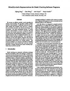
The transition relation specifies the possible transitions from state to state, triggered by the applications of inputs to the system. For technical reasons, it is required to be total, i.e. for each state there exists at least a successor state. From such a tuple, abstracting away from inputs, one can immediately extract a state transition graph, a Kripke structure that only describes transitions from states to states.

A

C

B

A A

B

C

C

C

Fig. 1. A State Transition Graph and its unwinding.

A path in such a Kripke structure is obtained starting from a state s ∈ S i , and then repeatedly appending states reachable through R; since inputs have been abstracted away, a path corresponds to the evolution of the system for some sequence of inputs. Given the totality of R, behaviors are infinite. Since a state can have more than one successor, the structure can be thought of as unwinding into an infinite tree, representing all the possible executions of the system starting from the initial states. Figure 1 shows a state transition graph and its unwinding from the initial (colored) state. A Kripke structure is typically associated with a set of propositions P, and with a labeling function that maps each state onto a truth assignment to such propositions. In the following, we assume that one truth assignment to the variables in P is associated to at most one state, and we write s |= p to indicate that a proposition p holds in a state s. Traditionally, two temporal logics are most commonly used for model checking, CTL and LTL [31]. Computation Tree Logic (CTL) is interpreted over the computation tree of the Kripke structure, while Linear Temporal Logic (LTL) is interpreted over the set of its paths. These two logics have incomparable expressive power, and differ in how they handle branching in the underlying computation tree: CTL temporal operators quantify over the paths departing from a given state, while LTL operators describe properties of all possible computation paths. Model checking is the problem of deciding whether a certain temporal formula ϕ holds in a given Kripke structure M (see [24] for a detailed overview). In the following we use the notation M |= ϕ. The first model checking algorithms used an explicit representation of the Kripke structure as a labeled, directed graph [21, 22, 45]. Explicit state model checking is based on the exploration of the Kripke structure based on the expansion and storage of individual states. Over the years, explicit state model checking has reached impressive performance (see for instance the SPIN model checker [38]). The key problem, however, is that explicit state techniques are subject to the so-called state explosion problem, i.e. they need to explore and store the states of the state tran-

a1 a2

a2 b1 b2

b2

1

0

Fig. 2. A BDD for the formula (a1 ↔ a2 ) ∧ (b1 ↔ b2 ).

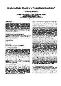
sition graph. In industrial sized systems, this amounts to an extremely large number of states. In fact, the Kripke structure is typically the result of the combination of a number of components (e.g. the communicating processes in a protocol), and the size of the resulting structure may be exponential in the number of components. A major breakthrough was enabled by the introduction of symbolic model checking [40]. In symbolic model checking, rather than individual states and transitions, the idea is to manipulate sets of states and transitions, using a logical formalism to represent the characteristic functions of such sets [26, 43, 52, 15]. Since a small logical formula may admit a large number of models, this results in most cases in a very compact representation which can be effectively manipulated. Each state is presented by an assignment to the propositions (variables) in P (equivalently, by the corresponding conjunction of literals). A set of states is represented by the disjunction of the formulae representing each of its states. The basic set theoretic operations (intersection, union, projection) are given by logical operations (such as conjunction, disjunction, and quantification). In the following we use x to denote the vector of variables representing the states of a given system; we write Si (x) for the formula representing the initial states. A similar construction can be applied to represent inputs (for which we use a vector of variables i). A set of “next” variables x0 is used for the state resulting after the transition: a transition from s to s0 is then represented as a truth assignment to the current and next variables. We use R(x, i, x0 ) for the formula representing the transition relation expressed in terms of those variables. Obviously, the key issue is the use of an efficient logical representation. The first one used for symbolic model checking was provided by Ordered Binary Decision Diagrams [12, 13] (BDDs for short). BDDs are a representation for boolean formulas, which is canonical once an order on the variables has been established. This allows equivalence checking in constant time. Figure 2 depicts the BDD for the boolean formula (a1 ↔ a2 ) ∧ (b1 ↔ b2 ), using the variable ordering a1 , a2 , b1 , b2 . Solid lines represent “then” arcs (the corresponding variable has to be considered positive), dashed lines

represent “else” arcs (the corresponding variable has to be considered negative). Paths from the root to the node labeled with “1” represent the satisfying assignments of the represented boolean formula (e.g., a1 ← 1, a2 ← 1, b1 ← 0, b2 ← 0). Such a powerful logical computation machinery provides the ideal basis for the implementation of algorithms manipulating sets of states. In fact, the use of BDDs makes it possible to verify very large systems (larger than 1020 states [15, 40, 14]). Symbolic model checking has been successful in various fields, allowing the discovery of design bugs that were very difficult to highlight with traditional techniques. For instance, in [23] the authors discovered previously undetected and potential errors in the design of the cache coherence protocol described in the IEEE Futurebus+ Standard 896.1.1991, and in [29] the cache coherence protocol of the Scalable Coherent Interface, IEEE Standard 1596-1992 was verified, finding several errors. A more recent advance in the field originates from the introduction of bounded model checking (BMC) [7, 6]. The idea is twofold. First, we look for a witness to a property violation that can be presented within a certain bound, say k transitions. Second, we generate a propositional formula that is satisfiable if and only if a witness to the property violation exists. The formula is obtained by unwinding the symbolic description of the transition relation over time. In particular, we use k + 1 vectors of state variables x0 , . . . , xk , whose assignments represent the states at the different steps, and k vectors of input variables i1 , . . . , ik , that represent the inputs at the different transitions: Si (x0 ) ∧ R(x0 , i1 , x1 ) ∧ . . . ∧ R(xk−1 , ik , xk ) Additional constraints are used to limit such assignments to witness the violation of the property, and to impose a cyclic behaviour when required. The solution technique leverages the power of modern SAT solvers [30], which are able to check the satisfiability of formulae with hundreds of thousands of variables, and millions of clauses. In comparison to BDD-based algorithms, the advantages of SAT-based techniques are twofold [25]. First, SAT-based algorithms have higher capacity, i.e. they can deal with a larger number of variables. Second, SAT solvers have a high degree of automation, and are less sensitive than BDDs to the specific parameters (e.g. variable ordering). As a result, SAT-based technologies have been introduced in industrial settings to complement and often to replace BDD-based techniques. In addition, SAT has become the core of many other algorithms and approaches, such as inductive reasoning (e.g. [50]), incremental bounded model checking (e.g. [36]), and abstraction (e.g. [35]). A survey of the recent developments can be found in [44].

3 Safety Analysis The goal of safety analysis is to investigate the behavior of a system in degraded conditions, that is, when some parts of the system are not working properly, due to malfunctions. Safety analysis includes a set of activities, that have the goal of identifying all possible hazards of the system, and that are performed in order to ensure that the system meets the safety requirements that are required for its deployment and use. Safety analysis activities are particularly critical in the case of reactive systems, because hazards can be the result of complex interactions involving the dynamics of the system [51].

Traditionally, safety analysis activities have been performed manually. Recently, there has been a growing interest in model-based safety analysis using formal methods [11, 9, 1, 10] and in particular symbolic model checking. Model-based safety analysis is carried out on formally specified models which take into account system behavior in the presence of malfunctions, that is, possible faults of some components. Symbolically, the occurrence of such faults is modeled with a set of additional propositions, called failure mode variables. Intuitively, a failure mode variable is true when the corresponding fault has occurred in the system (different failure mode variables are associated to different faults). In the rest of this section, we assume to have a system M = hS, Si , I, Ri with a set of failure mode variables F ⊆ P. Furthermore, for the sake of simplicity, we assume that failure modes are permanent (once failed, always failed), that is, we assume that the following condition holds: ∀f ∈ F, s1 , s2 ∈ S, i ∈ I

(hs1 , i, s2 i ∈ R ∧ s1 |= f ) ⇒ s2 |= f

(1)

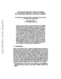
The theory can be extended to the more general case of sporadic or transient failure modes, that is, when faults are allowed to occur sporadically (e.g., a sensor showing an invalid reading for a limited period of time), possibly repeatedly over time, or when repairing is possible. In this section we briefly describe two of the most popular safety analysis activities, that is, fault tree analysis (FTA) and failure mode and effect analysis (FMEA), and we discuss their relationship with the symbolic model checking techniques illustrated in Section 2. Fault Tree Analysis [53] is an example of deductive analysis, which, given the specification of an undesired state, usually referred to as a top level event, systematically builds all possible chains of one of more basic faults that contribute to the occurrence of the event. The result of the analysis is a fault tree, that is, a representation of the logical interrelationships of the basic events that lead to the undesired state. In its simpler form (see Fig. 3) a fault tree can be represented with a two-layer logical structure, namely a top level disjunction of the combinations of basic faults causing the top level event. Each combination, which is called cut set, is in turn the conjunction of the corresponding basic faults. In general, logical structures with multiple layers can be used. A cut set is formally defined via CTL as follows. Definition 2 (Cut set). Let M = hS, Si , I, Ri be a system with a set of failure mode variables F ⊆ P, let FC ⊆ F be a fault configuration, and TLE ∈ P a top level event. We say that FC is a cut set of TLE, written cs(FC, TLE) if ^ ^ M |= EF ( f ∧ ¬f ∧ TLE). f ∈FC

f ∈(F\FC)

Intuitively, a fault configuration corresponds to the set of active failure mode variables. Typically, among the possible fault configurations, one is interested in isolating those that are minimal in terms of failure mode variables, that is, those that represent simpler explanations, in terms of system faults, for the occurrence of the top level event. Under the hypothesis of independent faults, these configurations also represent the most probable explanations for the top level event, and therefore they have a higher importance in reliability analysis. Minimal configurations are called minimal cut sets and are formally defined as follows.

Fig. 3. An example of fault tree

Definition 3 (Minimal Cut Sets). Let M = hS, Si , I, Ri be a system with a set of failure mode variables F ⊆ P, let F = 2F be the set of all fault configurations, and TLE ∈ P a top level event.We define the set of cut sets and minimal cut sets of TLE as follows: CS(TLE) = {FC ∈ F | cs(FC, TLE)} MCS(TLE) = {cs ∈ CS(TLE) | ∀cs0 ∈ CS(TLE) (cs0 ⊆ cs ⇒ cs0 = cs)} As a side remark, we mention that the notion of minimal cut set can be extended to the more general notion of prime implicant (see [27]). The notion of prime implicants is based on a different definition of minimality, involving both the activation and the absence of faults (we refer to [27] for more details). Formally, the previous definition for MCS(TLE) needs to be modified to take into account the different notion of minimality. We also notice that, compared to the case of purely combinational systems, here failure mode variables may be associated to dynamics, and thus it is possible that different models of failure (e.g. persistent vs sporadic) may have different impact on the results. Moreover, the temporal relationships between failures may be important, e.g. a certain top level event may require f1 to occur before f2 . There have been proposals to enrich the notion of minimal cut set with such information [1]. Based on the previous definitions, fault tree analysis can therefore be described as the activity that, given a top level event, involves the computation of the (minimal) cut sets (or prime implicants) and their arrangement in the form of a tree. An example of fault tree, generated with the FSAP safety analysis platform [33], is shown in Fig. 3. Fault trees with multiple layers can also be obtained, for instance based on the hierarchy of the system model (see [2]).

Failure mode and effect analysis is similar to fault tree analysis. It takes as input a set of fault configurations and a set of top level events, and it produces a table mapping elements in the two sets. An entry in the table means that a given fault configuration is a possible explanation for the corresponding top level event. The formal definition is as follows. Definition 4 (Failure Mode and Effect Analysis). Let M = hS, Si , I, Ri be a system with a set of failure mode variables F ⊆ P, let F = {FC 1 , . . . , FC n } ⊆ 2F be a set of fault configurations, and T = {TLE 1 , . . . , TLE m } ⊆ P be a set of top level events. An FMEA table for F and TLE, denoted FMEA(F, T ) is the set of pairs {hFC i , TLE j i | cs(FC i , TLE j )}. Both FMEA and FTA can be realized with model checking techniques, as witnessed by the FSAP platform [33, 10]. As advocated in [11], it is important to have a complete decoupling between the system model and the fault model. For this reason, the FSAP platform relies on the notions of nominal system model and extended system model. The nominal model formalizes the behavior of the system when it is working as expected, whereas the extended model defines the behavior of the system in presence of faults. The decoupling between the two models is achieved in the FSAP platform by generating the extended model automatically via a so-called model extension step. The model extension step takes as input a system and a specification of the faults to be added, and automatically generates the corresponding extended system. It can be formalized as follows. Let M = hS, Si , I, Ri be the nominal system model. A fault is defined by the proposition p ∈ P to which it must be attached to, and by its type, specifying the “faulty behavior” of proposition p in the extended system (e.g., p can non-deterministically assume a random value, or p is stuck at a particular value). Given the proposition p, FSAP introduces a new proposition pFM , the failure mode variable, modeling the possible occurrence of the fault, and two further propositions p F ailed and pExt , with the following intuitive meaning. The proposition pF ailed models the behavior of p when a fault has occurred. For instance, the following condition (where S 0 is the set of states of the extended system) defines a so-called inverted failure mode (that is, proposition pF ailed holds if and only if proposition p does not hold): ∀s ∈ S 0

(2)

(s |= pF ailed ⇐⇒ s 6|= p)

The proposition pExt models the extended behavior of p, that is, it behaves as the original p when no fault is active, whereas it behaves as pF ailed in presence of a fault. Formally, we impose the following conditions: ∀s ∈ S 0 ∀s ∈ S

0

s |= p

s 6|= pFM ⇒ (s |= pExt ⇐⇒ s |= p)

(3)

FM

(4)

⇒ (s |= p

Ext

⇐⇒ s |= p

F ailed

)

The extended system MExt = hS 0 , Si0 , I, R0 i can therefore be easily defined in terms of the nominal system by adding the set of propositions {pFM , pF ailed , pExt } to the original set P, modifying the definition of the (initial) states and of the transition relation, and imposing the additional conditions (1), (2) (in the hypothesis of an inverted

failure mode), (3) and (4). We omit the details for the sake of simplicity. Finally, system extension with respect to a set of propositions can be defined in a straightforward manner, by iterating system extension over single propositions. The extended system model resulting from the extension step is used in FSAP to carry out the safety analysis activities, FMEA and FTA. The corresponding algorithms are implemented as an extension of the NuSMV tool [41, 16], a symbolic model-checker developed at ITC-IRST. As far as FTA is concerned, the FSAP platform can be used to compute both the minimal cut sets and the prime implicants of a given top level event. The computation involves two different stages, both of them relying on symbolic techniques. The first stage consists in computing the set of cut sets, that is, the set of fault configurations satisfying the condition of Def. 2. This can be realized, as described in [10], by using model checking symbolic techniques to compute a forward fixpoint of a forward image primitive. The second stage of the computation consists in extracting the set of minimal cut sets from the set computed at the previous stage. The extraction is based on classical routines for computing the prime implicants of Boolean functions [27, 46].

4 Diagnosis and Diagnosability Rarely physical systems are fully observable: parts of their state are hidden, and sensors are used to expose (partial) information about otherwise unobservable aspects. Diagnosis starts from observed run time behavior of a system, and tries to provide an explanation (in terms of hidden states). In particular, diagnosis is often the problem of identifying the set of possible causes of a specific unexpected or faulty behavior. The seminal approaches to diagnosis are carried out considering combinational, state-less models. These can be symbolically represented as a propositional formula Φ(x, o), where x are the hidden variables, and o are the observable variables (e.g. conveyed inputs and observed outputs). Within this framework, it is possible to encompass problems such as fault detection (that is, detecting whether the system is malfunctioning) and fault isolation (i.e. detecting a specific cause of malfunctioning). Let µ(o) denote an assignment to the observable variables. Then, we say that an assignment D(x) is a diagnosis (alternatively, an explanation) for µ(o) if Φ(x, o) is true under the interpretation µ(o) ∪ D(x). Notice that diagnoses need not be total, i.e. some hidden variables may be unassigned (in which case any extension to D(x) is also an explanation). In general, several possible explanations may exist, and some may be preferable over others, according to some criterion. For example, an explanation may be minimal (i.e. any of its subsets is not an explanation); alternatively, it could be of least cardinality, based on the number of assigned literals, or could be required to have the least number of variables assigned to true. Probabilistic information can be taken into account, in order to require the most likely explanation. In contrast to model checking and safety analysis, that are typically carried out at design time, diagnosis deals with the run-time of a system. Thus, we reject the assumption (that is used for for verification and safety analysis) that the system is fully observable. When considering the problem of diagnosis for reactive systems, failure

modes and other hidden variables may have their own dynamics, leading to the following extension of Def. 1: Definition 5 (Partially Observable System). A system is a tuple M hS, Si , I, O, R, X i where: – – – – – –

=

S is a finite set of states, Si ⊆ S is the set of initial states, I is a set of inputs to the system, R ⊆ S × I × S is the transition relation O is a set of possible observations; X ⊆ S × O is the observation relation;

We require X to be total, i.e. for each state s there exists an observation o such that X (s, o). Two states associated to the same observation may be indistinguishable. Notice that this model of observation is extremely expressive, as it makes it possible for a state to be associated to many different observations. The symbolic representation used in previous sections can be generalized to deal with the new notions. In particular, the set of observations O is presented symbolically by introducing a set of observation variables; each observation is represented by a valuation to the observation variables. The observation relation is then represented as a formula in the state variables and the observation variables. Definition 6. An execution in M is a sequence σ = s0 , o0 , i1 , s1 , o1 , i2 , . . . , ik , sk , ok , such that s0 ∈ S0 , R(si−1 , ii , si ) for 1 ≤ i ≤ k, and X (si , oi ) for 0 ≤ i ≤ k. The w observable trace of an execution σ is w = o0 , i1 , o1 , . . . , ik , ok , and we write σ : s0 −→ w sk . We also write s0 −→ sk if such a σ exists. The above definition captures the dynamics of a plant and its observable counterpart. If an execution σ has k steps, then it is associated to a trace w ∈ O × (I × O) k . The set of traces is in general a subset of O × (I × O)∗ . In the following we use σ to denote a feasible execution, and w to denote the corresponding (observable) trace. The problem of diagnosis in the setting of reactive systems generalizes the combinational case in the following directions. First, an explanation is no longer an assignment to the hidden variables, but rather an assignment to the hidden variables over time: in order to explain a sequence of length k, a suitable amount of assignments are in order. Second, the notion of preferable explanation may be generalized according to temporal aspects. As a result, there may be many more definitions of preference between explanations. Remarkably, given an observable trace w of specific length, it is possible to recast the problem of diagnosis within the framework of bounded model checking. In particular, we start from the formula describing all the executions of length k: Si (x0 ) ∧ X (x0 , o0 ) ∧ R(x0 , i1 , x1 ) ∧ X (x1 , o1 ) ∧ . . . ∧ R(xk−1 , ik , xk ) ∧ X (xk , ok ) We then restrict the set of models by conjoining it with the formula that restricts the input and output variables to assume the values required by the observable trace w: w[0] (o0 ) ∧ w[1] (i1 ) ∧ w[2] (o1 ) ∧ . . . ∧ w[2k−1] (ik ) ∧ w[2k] (ok )

where w[i] stands for the formula encoding the constraint expressed by i-th element of w. With this constraint, the input and output variables are assigned specific truth values: the formula resulting after the simplification only contains state variables, and the set of satisfying assignments to the (temporal instantiations of the) state variables is a description of the sequences of states that may be associated with the observable trace w. The problem of diagnosis has a design-time counterpart. In fact, it is often an important question whether a diagnoser will be able to carry out its tasks for all possible run-time executions of the observed system. This task, called diagnosability, can for instance be used in order to analyze the effectiveness and displacement of sensors in a design. The task of diagnosability has been tackled with several methods, based on automata theory and similar techniques, see e.g. [39, 48, 49]. Intuitively, a system is not diagnosable if two executions exist that share the same observable trace, but have different properties (e.g. in one a failure occurs, while the other one models a nominal behavior), and should be distinguishable. In [17], the problem is tackled by means of bounded model checking techniques, by reduction to a so-called twin model: Si (xl0 ) ∧ X (xl0 , o0 ) ∧ Si (xr0 ) ∧ X (xr0 , o0 )∧ l R(x0 , i1 , xl1 ) ∧ X (xl1 , o1 ) ∧ R(xr0 , i1 , xr1 ) ∧ X (xr1 , o1 ) ∧ . . . ∧ R(xlk−1 , ik , xlk ) ∧ X (xlk , ok ) ∧ R(xrk−1 , ik , xrk ) ∧ X (xrk , ok ) Two (left and right, l and r) copies of the system are fed with the same sequence of inputs, and forced to exhibit the same outputs. Additional constraints on the state variables are used to express the required properties of the left and right executions. If the problem is satisfiable, then the system is not diagnosable; in addition, it is possible to provide as diagnostic information the critical pair, i.e. the pair of indistinguishable executions. The usage of SMC techniques for this purpose has allowed checking the diagnosability of significantly complex system models developed within Nasa [17].

5 Planning We now introduce planning, and discuss its relationships with (symbolic) model checking and diagnosis. Planning is the problem of identifying a plan whose execution controls the system (called in that context planning domain) so that, when the system executes under the control of the plan, certain properties (over its states) are obeyed. Several specializations of this general statement are possible and relevant, both theoretically and for practical purposes. For instance, in classical planning [32, 34] it is assumed that the domain is deterministic, that its state can be observed at runtime, and that the desired execution properties amount to a set of goal states which must be finally reached. The deterministic nature of the controlled system allows restricting to plans structured simply as sequences of inputs that must be provided to the domain. In strong planning [20], the assumption that the domain is deterministic is removed. This makes it necessary to consider plans that have a conditional, loop-free structure, and that branch depending on the currently observed system state. Loops are also considered by a relaxation of

the problem called strong cyclic planning [18]. These same problems can be considered when the hypothesis of full observability of the domain is removed. In conformant planning [19], the opposite hypothesis is made: nothing can ever be observed about the status of the domain; therefore, plans may not branch and have a sequential structure like in classical planning. In this case, however, goal achievement has to be guaranteed regardless of nondeterminism - i.e. several different, but equally plausible executions must be considered for the plan. Contingent planning [8, 5] deals with the more general case where a domain is partially observable, i.e. it has the same features of the systems considered for diagnosis in Section. 4. On top of having to consider multiple executions, of course, contingent plans have a branching structure, and take choices at runtime depending on the currently perceived observations. Different planning problems have also been tackled where goals are not anymore set of states to be reached, but define constraints over the behavior of the domain during the whole plan execution, using CTL [42] or different logics [28]. In all instantiations of the planning problem, the plan can be interpreted as an automaton, whose execution controls the system (the planning domain) by synchronously reading the system’s outputs (the observations) and providing the system’s inputs (the planning actions). The specific plan structures considered in the various problems simply correspond to constraints over the structure of the corresponding automata. Thus planning refers to a framework where the system and diagnoser described in the previous sections are complemented by a controller (the plan). Here, we provide the most general definition, referring to a partially observable domain - its simplifications for the special cases of full or null observability are trivial. Definition 7 (controller). A controller for system M = hS, Si , I, O, R, X i is a tuple Π = hΣ, σ0 , α, i, where: – Σ is the set of contexts. – σ0 ∈ Σ is the initial context. – α : Σ × O * I is the action function; it associates to a context c and an observation o an input a = α(c, o) for the system. –  : Σ × O * Σ is the context evolution function; it associates to a context c and an observation o a new context c0 = (c, o). Naturally, a symbolic representation in terms of variables is also possible, and indeed used, for the controller as well as for the system. Notice that the controller is a deterministic Moore machine; nondeterministic controllers are not useful for our purposes and therefore we will not consider them. The execution of the system under the control of the plan can be represented by a Kripke structure, called execution structure, whose states are configurations that couple system states and plan contexts. In fact, the execution structure is a finite presentation of every possible execution trace, and corresponds to the standard synchronous product of the plan and the system, denoted M × Π. This makes it possible to define a notion of satisfactory plan, for some property φ, in terms of a model checking problem: plan Π satisfies goal φ for domain M if and only if M × Π |= φ. When the goal φ is expressed as a CTL or LTL formula, standard model checking techniques can be used for this purpose.

Therefore, the planning problem can be formulated as follows: given a system M and a goal φ, find an executable controller Π such that their synchronous execution satisfies the goal φ, i.e. Π × M |= φ. This statement highlights the main differences and similarities between planning and model checking: they both refer to properties of execution of a system modeled as a finite state automata (eventually constrained by a controller), but the latter is a synthesis problem rather than a verification one. In general, planning is a (theoretically and practically) harder problem than model checking, which intuitively requires searching for a single execution witness, rather than for a complex plan. The fact that model checking also synthesizes a counterexample for a non-valid property makes it possible to exploit it in a direct way to solve planning problems in the specific ’classical’ setting. This is performed by stating, as the property that needs be verified, that the goal φ can never be finally achieved. As usual, the application of model checking returns one of two possible answers: either such property holds, or it does not and a counterexample is given. In the former case, this indicates that it is actually impossible to achieve the goal, therefore no plan exists. In the latter, a plan exists, and it corresponds to the sequence of inputs given as a counterexample. For more complex cases, such a direct usage of model checking to generate solution controllers is not possible, either because controllers have a branching/looping structure or because the goal language must be richer then the CTL/LTL used in model checking. In these cases, the commonalities between the elements involved in model checking and planning are exploited by making use of model checking’s symbolic techniques and primitives to manipulate planning domains. For instance, strong planning under full observability can be tackled by a backward fixpoint of a backward image primitive. Such strong backward image must be defined to derive all the strong predecessors of a set of states φ, i.e. all those states such that there exists some action whose outcomes, applied to them, all belong to φ. This primitive can be defined as a QBF formula and implemented on top of the basic BDD primitives used to compute the semantics of the temporal CTL formula AXφ in model checking. Similar primitives are adopted for the remaining planning problems: in every case, the ability to manipulate sets of states by means of basic primitives is used to describe (forward/backward) images either on search frontiers, or on sets of observationally equivalent states. Concerning the relationships between diagnosis and planning, they are evident once partially observable domains are considered. In this case, as stated in [4], CTL is not adequate to express many interesting planning goals. Such inadequacy is related with the fact that in this setting, during plan execution, a monitor has only limited run-time information, which in general is not sufficient to rule out uncertainty about the state of the controlled system. To express that a certain property must not only be achieved, but also detected by the monitor, the knowledge operator K must be added to CTL, i.e. the K-CTL logic developed for diagnosis is adopted. For instance, a strong requirement of the form “finally achieve and detect property φ”, such as those considered in most contingent planning approaches ([5, 47, 37]), can be written as the K-CTL formula AF K φ. That is, those approaches solve the problem of identifying a controller Π such that

M × Π |= AF K φ Two remarks are in order. First, as discussed in [3], considering CTL goals may nevertheless be interesting in some cases, where goal detection is not possible, and only goal achievement can be pursued. Second, symbolic model checking techniques can also be used when looking for plans that satisfy K-CTL goals. For this purpose one needs to consider the search space called belief space, whose nodes are sets of observationally equivalent states called beliefs, representing the epistemic knowledge of a universal monitor. Contingent planning on K-CTL goals can be formulated as and/or search in the belief space [8], and, as shown in [5, 47], it is possible to represent beliefs symbolically, as formulas modeling sets of states, and progress or regress them by appropriate image primitives. The relationship between diagnosability and (contingent) planning becomes evident when a K-CTL goal formula of the form AF (K(φ) ∨ K(¬φ)) is used. In this case, the generated plan is one that finally achieves knowing whether φ holds or not, i.e. diagnosing φ. That is, contingent planning is to diagnosability what classical planning is to model checking: it generates a controller that drives the system to achieve a goal that can be otherwise verified by a diagnosability check. This paves the way to the use of K-CTL planning to generate active diagnosers, that is controllers that can be used to appropriately drive systems so that faults can be discovered. Notice the major difference with the passive diagnosing of Section 4: here, we are not given the execution trace for diagnosing, but rather we generate from scratch a controller that - interacting with the system in a non trivial way - drives it so that the observer will obtain a univocal diagnosis. We also remark that the generality of the approach allows conjoining “diagnosis-oriented” goals such as the above with different requirements; e.g a formula of the form AF φ actually forces the system to finally achieve φ, and a formula of the form AGψ requires that ψ holds throughout the execution of the plan. This way, we obtain a controller that conjoins a diagnosis task with a control task that aims at driving the system according to some desirable behavior. The way in which the different tasks are mixed within a unique controller is responsibility of the specific and/or search algorithm used to visit the belief space, and in particular of search heuristics. By now, we conducted some preliminary experiments with active diagnosis by enriching the goal language of the MBP system with the modal knowledge operator, and leaving implicit - as usual - the top-level CTL AF operator. We conducted the experiments on a model of the Cassini spacecraft and we were able to synthesize a diagnoser for several goals of the form AF (K(φ) ∨ K(¬φ)). We implemented a prototype, based on MBP, which is able to synthesize the diagnoser for the given goal and to automatically generate the model corresponding to the synchronous product of the synthesized controller and the original model. The diagnosability properties of the resulting model were further verified using the FSAP platform [33].

6 Conclusions and Future Work In this paper we have discussed how the framework of symbolic model checking can be used to model several interesting problems for the development of reactive systems: safety analysis, diagnosis, diagnosability, and synthesis. Symbolic model checking also provides effective computational primitives and tools for the implementation of special purpose, highly effective algorithms to tackle the above problems. We believe that one of the most interesting challenges in the field is to provide an effective support toolset, where different design tasks can be cast in a uniform working framework.

References ˚ 1. O. Akerlund, P. Bieber, E. B¨oede, M. Bozzano, M. Bretschneider, C. Castel, A. Cavallo, M. Cifaldi, J. Gauthier, A. Griffault, O. Lisagor, A. L¨udtke, S. Metge, C. Papadopoulos, T. Peikenkamp, L. Sagaspe, C. Seguin, H. Trivedi, and L. Valacca. ISAAC, a framework for integrated safety analysis of functional, geometrical and human aspects. In Proc. European Congress on Embedded Real Time Software (ERTS 2006), 2006. 2. R. Banach and M. Bozzano. Retrenchment, and the Generation of Fault Trees for Static, Dynamic and Cyclic Systems. In J. Gorski, editor, Proc. Conference on Computer Safety, Reliability and Security (SAFECOMP 2006), volume 4166 of LNCS, pages 127–141. Springer, 2006. 3. P. Bertoli, A. Cimatti, and M. Pistore. Strong Cyclic Planning under Partial Observability. In Proc. of 17th European Conference on Artificial Intelligence (ECAI 2006), 2006. 4. P. Bertoli, A. Cimatti, M. Pistore, and P. Traverso. A Framework for Planning with Extended Goals under Partial Observability. In Proc. International Conference on Automated Planning and Scheduling (ICAPS 2003), 2003. 5. P. Bertoli, A. Cimatti, M. Roveri, and P. Traverso. Strong Planning under Partial Observability. Artificial Intelligence, 170:337–384, 2006. 6. A. Biere, A. Cimatti, E. Clarke, M. Fujita, and Y. Zhu. Symbolic Model Checking Using SAT Procedures instead of BDDs. In Proceedings of the 36th Design Automation Conference (DAC’99), pages 317–320, New Orleans, LA, USA, June 1999. ACM Press. 7. A. Biere, A. Cimatti, E. Clarke, and Y. Zhu. Symbolic model checking without BDDs. In R. Cleaveland, editor, Proceedings of the Fifth International Conference on Tools and Algorithms for the Construction and Analysis of Systems (TACAS’99), volume 1579 of Lecture Notes in Computer Science, pages 193–207. Springer Verlag, 1999. 8. B. Bonet and H. Geffner. Planning with Incomplete Information as Heuristic Search in Belief Space. In Proc. 5th International Conference on Artificial Intelligence Planning and Scheduling (AIPS 2000), pages 52–61, 2000. 9. M. Bozzano, A. Cavallo, M. Cifaldi, L. Valacca, and A. Villafiorita. Improving Safety Assessment of Complex Systems: An industrial case study. In K. Araki, S. Gnesi, and D. Mandrioli, editors, Proc. Formal Methods Europe Symposium (FM 2003), volume 2805 of LNCS, pages 208–222. Springer, 2003. 10. M. Bozzano and A. Villafiorita. The FSAP/NuSMV-SA Safety Analysis Platform. International Journal on Software Tools for Technology Transfer, 2006. DOI 10.1007/s10009-0060001-2. To appear. ˚ 11. M. Bozzano, A. Villafiorita, O. Akerlund, P. Bieber, C. Bougnol, E. B¨ode, M. Bretschneider, A. Cavallo, C. Castel, M. Cifaldi, A. Cimatti, A. Griffault, C. Kehren, B. Lawrence, A. L¨udtke, S. Metge, C. Papadopoulos, R. Passarello, T. Peikenkamp, P. Persson, C. Seguin,

12. 13. 14. 15. 16.

17.

18. 19. 20. 21. 22. 23.

24. 25.

26.

27.

L. Trotta, L. Valacca, and G. Zacco. ESACS: An Integrated Methodology for Design and Safety Analysis of Complex Systems. In Proc. European Safety and Reliability Conference (ESREL 2003), pages 237–245. Balkema Publisher, 2003. R. E. Bryant. Graph-Based Algorithms for Boolean Function Manipulation. IEEE Transactions on Computers, C-35(8):677–691, August 1986. R. E. Bryant. Symbolic Boolean Manipulation with Ordered Binary-Decision Diagrams. ACM Computing Surveys, 24(3):293–318, September 1992. J. R. Burch, E. M. Clarke, D. E. Long, K. L. McMillan, and D. L. Dill. Symbolic Model Checking for Sequential Circuit Verification. IEEE Transactions on Computer-Aided Design of Integrated Circuits and Systems, 13(4):401–424, April 1994. J. R. Burch, E. M. Clarke, K. L. McMillan, D. L. Dill, and L. J. Hwang. Symbolic Model Checking: 1020 States and Beyond. Information and Computation, 98(2):142–170, June 1992. A. Cimatti, E.M. Clarke, E. Giunchiglia, F. Giunchiglia, M. Pistore, M. Roveri, R. Sebastiani, and A. Tacchella. NuSMV2: An OpenSource Tool for Symbolic Model Checking. In E. Brinksma and K.G. Larsen, editors, Proc. Conference on Computer Aided Verification (CAV 2002), volume 2404 of LNCS, pages 359–364. Springer, 2002. A. Cimatti, C. Pecheur, and R. Cavada. Formal Verification of Diagnosability via Symbolic Model Checking. In G. Gottlob and T. Walsh, editors, Proceedings of the International Joint Conference on Artificial Intelligence (IJCAI’03), pages 363–369, Acapulco, Mexico, 2003. Morgan Kaufmann. A. Cimatti, M. Pistore, M. Roveri, and P. Traverso. Weak, Strong, and Strong Cyclic Planning via Symbolic Model Checking. Artificial Intelligence, 147(1-2):35–84, 2003. A. Cimatti, M. Roveri, and P. Bertoli. Conformant Planning via Symbolic Model Checking and Heuristic Search. Artificial Intelligence, 159:127–206, 2004. A. Cimatti, M. Roveri, and P. Traverso. Strong Planning in Non-Deterministic Domains via Model Checking. In Proc. 4th International Conference on Artificial Intelligence Planning Systems (AIPS-98), Carnegie Mellon University, Pittsburgh, USA, June 1998. AAAI-Press. E. M. Clarke and E. A. Emerson. Synthesis of Synchronization Skeletons for Branching Time Temporal Logic. In Logic of Programs: Workshop, volume 131 of Lecture Notes in Computer Science. Springer Verlag, May 1981. E. M. Clarke, E. A. Emerson, and A. P. Sistla. Automatic Verification of Finite-State Concurrent Systems using Temporal Logic Specifications. ACM Transactions on Programming Languages and Systems, 8(2):244–263, 1986. E. M. Clarke, O. Grumberg, H. Hiraishi, S. Jha, D. Long, K. L. McMillan, and L. Ness. Verification of the FUTUREBUS+ Cache Coherence Protocol. In Proc. of 11th International Symposium on Computer Hardware Description Languages and their Applications (CHDL93), 1993. E. M. Clarke, O. Grumberg, and D. Peled. Model Checking. MIT Press, Cambridge, MA, 1999. F. Copty, L. Fix, R. Fraer, E. Giunchiglia, G. Kamhi, A. Tacchella, and M. Y. Vardi. Benefits of bounded model checking at an industrial setting. In Proc. 12th Intl. Conference on Computer Aided Verification (CAV’01), Lecture Notes in Computer Science, pages 436–453, 2001. O. Coudert, C. Berthet, and J. C. Madre. Verification of Synchronous Sequential Machines Using Symbolic Execution. In Proc. of International Workshop on Automatic Verification Methods for Finite State Systems, volume 407 of Lecture Notes in Computer Science, pages 365–373, Grenoble, France, June 1989. Springer-Verlag. O. Coudert and J. C. Madre. Fault Tree Analysis: 1020 Prime Implicants and Beyond. In Proc. Annual Reliability and Maintainability Symposium (RAMS 1993), 1993.

28. U. Dal Lago, M. Pistore, and P. Traverso. Planning with a Language for Extended Goals. In Proc. 18th National Conference on Artificial Intelligence (AAAI’02), 2002. 29. D. L. Dill, A, J. Drexler, A. J. Hu, and C. H. Yang. Protocol Verification as a Hardware Design Aid. In International Conference on Computer Design, VLSI in Computers and Processors, pages 522–525, Los Alamitos, Ca., USA, October 1992. IEEE Computer Society Press. 30. N. E`en and N. S¨orensson. An extensible sat solver. In Proc. of the 6th International Conference on Theory and Applications of Satisfiability Testing, pages 502–518, 2003. 31. E. Emerson. Temporal and Modal Logic. In Handbook of Theoretical Computer Science, Vol. B: Formal Models and Semantics. Elsevier, 1990. 32. R. E. Fikes and N. J. Nilsson. STRIPS: A New Approach to the Application of Theorem Proving to Problem Solving. Artificial Intelligence, 2:187–208, 1971. 33. The FSAP platform. http://sra.itc.it/tools/FSAP. 34. M. Ghallab, D. Nau, and P. Traverso. ”Automated Planning: Theory and Practice”, chapter 1, pages 17–110. ”Morgan Kaufmann”, 2004. 35. A. Gupta, E. Clarke, and O. Strichman. Sat based counterexample-guided abstractionrefinement. IEEE Transactions on Computer Aided Design, 23:1113–1123, 2004. 36. K. Heljanko, T. A. Junttila, and T. Latvala. Incremental and complete bounded model checking for full PLTL. In Proc. of the 17th Int. Conf. on Computer Aided Verification (CAV’05), volume 3576 of LNCS, pages 98–111. Springer, 2005. 37. J¨org Hoffmann and Ronen Brafman. Contingent Planning via Heuristic Forward Search with Implicit Belief States. In Proc. of 15th International Conference on Automated Planning and Scheduling (ICAPS-05), pages 71–80, Monterey, CA, USA, 2005. Kaufmann. 38. G. J. Holzmann. The model checker Spin. IEEE Trans. on Software Engineering, 23(5):279– 295, May 1997. Special issue on Formal Methods in Software Practice. 39. S. Jiang, Z. Huang, V. Chandra, and R. Kumar. A polynomial algorithm for testing diagnosability of discrete event systems. IEEE Transactions on Automatic Control, 46(8):1318– 1321, August 2001. 40. K. L. McMillan. Symbolic Model Checking. Kluwer Academic Publ., 1993. 41. The NuSMV model checker. http://nusmv.itc.it. 42. M. Pistore and P. Traverso. Planning as Model Checking for Extended Goals in Nondeterministic Domains. In Proc. of 17th International Joint Conference on Artificial Intelligence (IJCAI-01), 2001. 43. C. Pixley. A Computational Theory and Implementation of Sequential Hardware Equivalence. In DIMACS Workshop on Computer Aided Verification ’90, pages 293–320, Providence, RI, 1990. 44. M. Prasad, A. Biere, and A. Gupta. A survey of recent advances in sat-based formal verification. STTT, (7):156–173, 2005. 45. J. P. Queille and J. Sifakis. Specification and Verification of Concurrent Systems in CESAR. In Proc. 5th International Symposium on Programming, Lecture Notes in Computer Science, Vol. 137, pages 337–371. SV, Berlin/New York, 1982. 46. A. Rauzy. New Algorithms for Fault Trees Analysis. Reliability Engineering and System Safety, 40(3):203–211, 1993. 47. J. Rintanen. Backward Plan Construction for Planning as Search in Belief Space. In Proc. of 6th International Conference on Artificial Intelligence Planning and Scheduling (AIPS’02), pages 93–102, 2002. 48. M. Sampath, R. Sengupta, S. Lafortune, K. Sinnamohideen, and D. Teneketzis. Diagnosability of discrete-event systems. IEEE Transactions on Automatic Control, 40(9):1555–1575, September 1995.

49. M. Sampath, R. Sengupta, S. Lafortune, K. Sinnamohideen, and D. Teneketzis. Failure diagnosis using discrete event models. IEEE Transactions on Control Systems, 4(2):105– 124, March 1996. 50. Mary Sheeran, Satnam Singh, and Gunnar Stalmarck. Checking safety properties using induction and a sat-solver. In Hunt and Johnson, editors, Proc. Int. Conf. on Formal Methods in Computer-Aided Design (FMCAD 2000), 2000. 51. N. O. Siu. Risk Assessment for Dynamic Systems: An Overview. Reliability Engineering and System Safety, 43:43–74, 1994. 52. H. J. Touati, H. Savoj, B. Lin, R. K. Brayton, and A. Sangiovanni-Vincentelli. Implicit State Enumeration of Finite State Machines Using BDDs. In Proc. of the IEEE International Conference on Computer-Aided Design, pages 130–133, Santa Clara, CA, November 1990. IEEE Computer Society Press. 53. W. E. Vesely, F. F. Goldberg, N. H. Roberts, and D. F. Haasl. Fault Tree Handbook. Technical Report NUREG-0492, Systems and Reliability Research Office of Nuclear Regulatory Research U.S. Nuclear Regulatory Commission, 1981.