Journal of Mathematical Biology manuscript No. (will be inserted by the editor)
Peter Clote · J¨ urg Straubhaar
Symmetric time warping, Boltzmann pair probabilities and functional genomics c Springer-Verlag 2006 Received: date / Revised version: date – ° Abstract. Given two time series, possibly of different lengths, time warping is a method to construct an optimal alignment obtained by stretching or contracting time intervals. Unlike pairwise alignment of amino acid sequences, classical time warping, originally introduced for speech recognition, is not symmetric in the sense that the time warping distance between two time series is not necessarily equal to the time warping distance of the reversal of the time series. Here we design a new symmetric version of time warping, and present a formal proof of symmetry for our algorithm as well as for one of the variants of Aach and Church [1]. We additionally design quadratic time dynamic programming algorithms to compute both the forward and backward Boltzmann partition functions for symmetric time warping, and hence compute the Boltzmann probability that any two time series points are aligned. In the future, with the availability of increasingly long and accurate time series gene expression data, our algorithm can provide a sense of biological Department of Biology, Courtesy appt. in Computer Science, Boston College, Chestnut Hill, MA 02467
[email protected] Department of Molecular Medicine, University of Massachusetts Medical School, Worcester, MA 01655
[email protected] Send offprint requests to: Peter Clote Key words: Time warping, Boltzmann partition function, gene expression data, time series
2
Peter Clote, J¨ urg Straubhaar
significance for aligned time points – e.g. our algorithm could be used to provide evidence that expression values of two genes have higher Boltzmann probability (say) in the G1 and S phase than in G2 and M phases. Public availability of our work is provided at bioinformatics.bc.edu/~clotelab/, which include a web server and Python source code.
1. Introduction
Functional genomics concerns the algorithmic determination of gene function, pursuant to high-throughput experimental assays, including methods using oligo and cDNA array expression chips. An early contribution to this field was made in 1998 by Eisen et al. [3], who used Pearson correlation coefficient of time series expression data for two genes as a measure of their similarity, and implemented average-linkage cluster analysis (a.k.a. the wellknown UPGMA1 phylogenetic tree construction algorithm, cf. text by Clote and Backofen [2]), to cluster cDNA microarray from S. cerevisiae. In 1998 Cho et al. [5] used Affymetrix arrays containing oligonucleotide sequences from 6218 genes of S. cerevisiae, and by measuring the logarithm of absolute expression levels at times 0,10,20,. . . ,160 minutes, representing roughly two yeast cell cycles, determined that 416 genes were regulated by cell cycle. More than 25% of the 416 genes were found to be adjacent to other genes induced in the same cell cycle phase. In 1998, using cDNA microarrays (in contrast to oligonucleotide arrays) Spellman et al. [4] extended and refined 1
UPGMA is an acronym for unweighted pair group method with arithmetic
mean.
Time warping and Boltzmann pair probabilities
3
the work of Cho et al. [5], by identifying 800 genes algorithmically determined to be regulated by cell cycle. Spellman et al. used procedures involving Fourier transform, Pearson correlation coefficient and average-linkage analysis of Eisen et al. Prior to [5, 4], only 104 yeast genes had been determined to be regulated by cell cycle, using traditional experimental methods. Later, Cho et al. [6] used Affymetrix oligonucleotide arrays to determine human cell cycle-regulated genes, by measuring the logarithm of the absolute expression levels at times 0,2,4,. . . ,24 hours, representing approximately two cell cycles of H. sapiens.
It is common practice to compute the Pearson correlation coefficient between two gene expression time series sequences [4], in order to determine putative functionally related genes. However, this requires that both sequences have the same length; in contrast, for sequences of unequal length, time warping can be used, as first noticed by Aach and Church [1]. Time warping is a kind of dynamic programming sequence alignment algorithm, where unlike the algorithm of Needleman and Wunsch [11] for global alignment or of Smith and Waterman [12] for local alignment, the sequences consist of real numbers instead of nucleotide or amino acid symbols. Aach and Church [1] implemented several variants of time warping algorithms first described in 1983 by Kruskal and Liberman [7] in the context of speech recognition. While Aach and Church focused principally on investigating the stability of time warping using the data set of Spellman et al. [4], in this paper, we propose a method to quantify the biological significance of
4
Peter Clote, J¨ urg Straubhaar
any two points from time series A and B, which are aligned in an optimal global time warping of series A with series B. Specifically, we introduce a new symmetric2 version of time warping, by modifying the time warping algorithm of Kruskal and Liberman [7]. We present a formal proof of symmetry for our algorithm, as well as that for one of the variants of Aach and Church [1].3 A technical advantage of any symmetric version of time warping is that it allows an unambiguous computation of the Boltzmann probability that two time series points are aligned in an optimal global time warping of gene expression values, given time series of possibly different lengths – this is analogous to the case of sequence alignment [13, 10, 9]. Along these lines, we design a dynamic programming algorithm to compute the forward and backward partition functions for our version of time warping, thus yielding the Boltzmann probability that any two time series points are aligned. We illustrate our algorithm, using gene expression time series for S. cerevisiae 2
By symmetric, we mean that the time warping distance between series A and
B equals that between series Ar and B r , where Ar resp. B r denotes the reversal of the series from last time point to first time point. While dynamic programming sequence alignment [11] has this property, classical time warping does not. 3
Aach and Church [1] did not originally notice that the time warping algo-
rithm implemented by their software genewarp with flag -a 2 is symmetric; i.e. genewarp.exe -i1 input1.txt -i2 input2.txt -a 2 -o out.txt . Since our proof of symmetry for genewarp -a 2 is similar to, but notationally different than the proof of symmetry for our new algorithm, for economy of space, we present the proof of symmetry of [1] in the appendix.
Time warping and Boltzmann pair probabilities
5
[5] and for H. sapiens [6], both approximately two cell cycles in duration. While this paper focuses on the new time warping algorithm, the formal proof of symmetry, and how to compute Boltzmann pair probabilities, a sequel will focus on applications, and investigate the relation between time warping, homology and function from the gene ontology (GO) database www.geneontology.org.
2. Classical time warping algorithm Time warping of two sequences a1 , . . . , an and b1 , . . . , bm , where each ai , bj ∈ Rk is a k-vector of features was introduced by Kruskal and Liberman in the context of speech recognition, where in the 1980’s, k was chosen between 6 and 15, and the ith component (or feature) was taken to be the “power present in a speech utterance in the ith frequency band at time t (using a short-time spectral analysis)” [7].4 Time warping is reminiscent and algorithmically similar, though distinct, to dynamic programming pairwise sequence alignment [2], where compression resp. expansion are analogous to sequence deletion resp. insertion. (One can easily imagine this situation when comparing a Texan drawl with a British accent, where in the former vowels may be drawn out while in the latter terminal syllables of words may be inaudible.) In [1], Aach and Church implemented variants of the KruskalLiberman algorithms for time warping and interpolated time warping for gene expression data analysis, where in some applications, k was chosen to 4
In this paper, unlike the approach of [1], k will always be taken to be 1;
nevertheless, all of our results hold for arbitrary k.
6
Peter Clote, J¨ urg Straubhaar
be large (e.g. 450), to accomodate a fixed sequence of genes taken together as features. Given time intervals τ, µ > 0, and sequences a = (a1 , . . . , an ) and b = (b1 , . . . , bm ) of elements of Rk , where ai resp. bj is the time series value at time (i − 1)τ resp. (j − 1)µ, consider functions u : {1, 2, . . . , T } → {1, . . . , n} and v : {1, 2, . . . , T } → {1, . . . , m}.5 Functions u, v are said to constitute a (discrete) time warping of a, b, provided that: 1. the boundary conditions u(1) = 1 = v(1), u(T ) = n, v(T ) = m hold. 2. u, v are monotonically increasing, though not necessarily strictly increasing, i.e. i ≤ j implies that u(i) ≤ u(j) and v(i) ≤ v(j). 3. u, v satisfy the continuity condition, i.e. u(i) ≤ u(i + 1) ≤ u(i) + 1, v(j) ≤ v(j + 1) ≤ v(j) + 1. For example, consider the time warping given in the left panel of Figure 1, where T = 9, n = 7, m = 6, and functions u, v are defined by the Table 1. The right panel of this figure depicts the corresponding path graph, which graphs the successive aligned positions {(u(i), v(i)) : 1 ≤ i ≤ T }.
Recalling that ai [resp. bj ] is the time series value at time (i − 1)τ [resp. (j − 1)µ] for 1 ≤ i ≤ n, 1 ≤ j ≤ m, one can identify ai with bj if u(t) = i 5
The definition we give is for equal interval time series, used in our application.
A more general definition of time warping for unequal interval time series can be found in [7] as well as in the algorithm of Aach and Church [1]; the latter is explained in the appendix.
Time warping and Boltzmann pair probabilities
7
7
6
5
4
3
2
t
1
2
3
4
5
6
7
8
9
u
1
1
2
3
4
5
5
6
7
v
1
2
3
3
3
4
5
6
6
1
0 0
1
2
3
4
5
6
7
8
Table 1. (Left) Time warpings u : {1, 2, . . . , T } → {1, . . . , n} and v : {1, 2, . . . , T } → {1, . . . , m}. (Right) Path graph for alignment induced by these time warpings.
and v(t) = j for some t ∈ {1, . . . , T }. For the example in Table 1, this yields the alignment in Figure 1, which is reminiscent of a trace for a pairwise sequence alignment. (See [14, 2] for more on traces and sequence alignment.) The difference between a time warping alignment and a trace lies in the fact that in a time warping, there are no skipped sequence elements – instead, multiple edges from the same sequence element indicate an expansion (e.g. Texan drawl of a vowel). In a trace, there are no muliple edges from the same element, and instead, skipped sequence elements correspond to gaps (insertions or deletions). Finally, time warping handles sequences of features, or elements of Rk , as opposed to sequences of amino acids or nucleotides.
Time warping distance was originally defined for the case of differentiable functions, where u0 resp. v 0 denotes the derivative of u resp. v with respect to time. The discrete analogogue is defined as follows.
8
Peter Clote, J¨ urg Straubhaar a1
a2
a3
a4
a5
a6
b1
b2
b3
b4
b5
b6
a7
Fig. 1. A time warping of a1 , . . . , a7 with b1 , . . . , b6 . Here, a1 is warped against both b1 and b2 , b3 is warped against a2 , a3 , a4 , etc.
Definition 1 (Kruskal-Liberman [7]). Suppose that a = (a1 , . . . , an ) and b = (b1 , . . . , bm ) are sequences of time series values in Rk , where ai resp. bj is the value at time (i − 1)τ resp (j − 1)µ, and let ρ : Rk × Rk → R+ be a given metric.6 If A is a time warping between a and b given by u : {1, . . . , T } → {1, . . . , n} and v : {1, . . . , T } → {1, . . . , m}, then the score of A, denoted S(A), is
T X ¡ ¢ (u(t) − u(t − 1)) · τ + (v(t) − v(t − 1)) · µ . ρ au(t) , bv(t) ) 2 t=1
Time warping distance between a and b is the minimum score, over all possible time warpings u : {1, . . . , T } → {1, . . . , n}, v : {1, . . . , T } → {1, . . . , m} between a and b. More intuitively, the time warping distance is the minimum score over all possible path graphs which satisfy the boundary, monotonicity and continuity conditions. An optimal time warping A between a and b is a time warping having minimum possible time warping score. 6
Recall that a metric, or distance function, ρ must satisfy the properties:
ρ(a, a) = 0, reflexivity ρ(a, b) = ρ(b, a), and triangle inequality ρ(a, c) ≤ ρ(a, b) + ρ(b, c). For instance, ρ could be Euclidean distance in Rk .
Time warping and Boltzmann pair probabilities
9
Notice that as in the case of sequence alignment, though time warping distance is uniquely defined, there may be more than one optimal time warping whose score equals the time warping distance. Following Definition 1, adapted from [7], classic time warping distance is computed by inductively computing Di,j to be the minimum time warping distance between a1 , . . . , ai and b1 , . . . , bj , for all 1 ≤ i ≤ n and 1 ≤ j ≤ m. Let D1,1 = 0, Di+1,1 = Di,1 + τ2 ρ(ai , b1 ), D1,j+1 = D1,j + µ2 ρ(a1 , bi ), and inductively define Di,j for 1 < i ≤ n, 1 < j ≤ m by
Di,j
Di−1,j−1 + τ +µ 2 · ρ(ai , bj ) = min Di−1,j + τ · ρ(ai , bj ) 2 Di,j−1 + µ · ρ(ai , bj ) 2
It follows that Dn,m is the optimal time warping distance between sequences a, b. Clearly, the corresponding dynamic programming algorithm requires space and time O(n · m). As illustrated in the right panel of Figure 1, a path graph for a time warping A of time series a1 , . . . , an and b1 , . . . , bm as follows. Place 1, 2, . . . , n along the x-axis and 1, 2, . . . , m along the y-axis. Whenever ai is warped in A against bj , a point is placed at coordinate (i, j). These coordinates are connected so that (i) if ai is warped against bj , bj+1 in A, then there is a vertical line segment from (i, j) to (i, j + 1), (ii) if ai , ai+1 is warped against bj in A, then there is a horizontal line segment from (i, j) to (i + 1, j), (iii) if ai is warped against bj and ai+1 is warped against bj+1 in A, then there
10
Peter Clote, J¨ urg Straubhaar
is a diagonal line segment from (i, j) to (i + 1, j + 1). A path graph for the time warping produced by Algorithm 1 is given in Figure 4. a1 b1
b2
a2
a3
a4
a5
-
a6
a7
b3
-
-
b4
b5
b6
-
Fig. 2. A trace of a1 , . . . , a7 with b1 , . . . , b6 , analogous to the time warping of Figure 1.
The classical notion of time warping distance, just introduced, is not symmetric, in the sense that time warping distance between a1 , . . . , an and b1 , . . . , bm is not necessarily the same as that between an , . . . , a1 and bm , . . . , b1 .7 In the context of speech recognition, which was the original context for the development of time warping algorithms [7], symmetric time warping is not reasonable because of the directionality of time in spoken words (ie drawing out syllables). This lack of symmetry in time warping is in contrast with ordinary sequence alignment, a feature used by [10, 9] (independently rediscovered by the first author) in order to define the Boltzmann probability P r[A] of sequence alignment A, as well as the Boltzmann probability of aligning amino acid ai with aj – the latter is given by the partition function of all alignments in which ai is aligned with aj divided by the partition function of all alignments. In this paper, by modifying classical time warping, we give an algorithm to compute symmetric time warping distance. After reading a preliminary version of this paper, J. Aach conjec7
i.e. time warping distance from left-to-right is not necessarily equal to that
from right-to-left.
Time warping and Boltzmann pair probabilities
11
tured that his algorithm genewarp [1] with flag -a 2 is symmetric as well. Here we prove the symmetry of our algorithm, and for economy of space, we prove Aach’s conjecture in the appendix. Additionally, we exploit the symmetry of our algorithm to design a dynamic programming algorithm to compute the forward and backward partition function, which then allows us to compute Boltzmann probabilities for the alignment of one time series point above another time series point. (Although we do not do so, one can similarly implement the partition function for genewarp with flag -a 2. We believe that time points from time series A and B which have large Boltzmann probability are biologically significant, in the same sense that Vingron and Argos [13] claimed a biological significance for certain regions of protein sequence alignments. Current gene expression data has far too few points to envision this approach to yield biological insights of the form, for instance, that certain yeast genes are better aligned in the G1 and S phase with certain other human genes than in the G2 and M phase of cell cycle. We feel that the design and implementation of our algorithm will provide a resource in the future when gene expression time series data sets are available with a greater number of time points. 3. Symmetric time warping . In this section, we describe a new symmetric time warping method in Algorithm 1, for which an inductive proof of symmetry is given. Before giving the pseudocode of the algorithm, we describe the underlying idea
12
Peter Clote, J¨ urg Straubhaar
to ensure symmetry. Recall that a time warping algorithm is defined to be symmetric if when given two numerical sequences a1 , . . . , an and b1 , . . . , bm , time warping distance is the same when computed left to right (using D i,j ) as when computed right to left (using Ei,j defined below). Equivalently time warping distance is the same between a1 , . . . , an and b1 , . . . , bm as between an , . . . , a1 and bm , . . . , b1 . Symmetry clearly holds for sequence alignment distance as computed by the Needleman-Wunsch algorithm [11]; however, symmetry does not hold for the classical time warping algorithm. Given numerical sequences a = a1 , . . . , an and b = b1 , . . . , bm , suppose that we have an optimal (partial) time warping of the subsequences a1 , . . . , ai and b1 , . . . , bj , for fixed i, j. To extend the time warping to the next number ai+1 and bj+1 from each sequence, three cases arise: (i) ai+1 is aligned with bj+1 , (ii) ai+1 is warped against bj , (iii) bj+1 is warped against ai . In particular, it can happen that the optimal time warping of a and b involves warping (say) bm against an−1 , leaving the last element an which must then be aligned with bm . In this hypothetical case, Dn,m = Dn−1,m +
τ 2
· ρ(an , bm ).
If we now consider time warping the sequences a and b from right to left, the first term, which compares an with bm is given by ρ(an , bm ). Compared with the last sentence of the previous paragraph, we are missing a multiplicative factor of τ2 . For this reason, in Algorithm 1, we pad a1 , . . . , an both on the left and on the right to produce a0 , a1 , . . . , an , an+1 , where a0 = a1 and an = an+1 , and similarly we pad the sequence b1 , . . . , bm on the left
Time warping and Boltzmann pair probabilities
13
and right to produce b0 , b1 , . . . , bm , bm+1 , where b0 = b1 and bm = bm+1 . Additionally, in cases of time expansion and compression, we interpolate values. Thus instead of the classical treatment of time expansion with term Di−1,j +
τ 2
· ρ(ai , bj ), we consider the term Di−1,j +
τ ρ(ai ,bj )+ρ(ai ,bj+1 ) . 2 2
Similarly, instead of the classical treatment of time compression with term Di,j−1 + µ2 ·ρ(ai , bj ), we consider the term Di,j−1 + µ2
ρ(ai ,bj )+ρ(ai+1 ,bj ) , 2
which
can be considered an attempt to interpolate or smooth out the transition. Our algorithm follows. Define D0,0 = 0 and for 1 ≤ i ≤ n and 1 ≤ j ≤ m, define Di,0 = Di−1,0 +
τ · ρ(ai , b0 ) 2
(1)
D0,j = D0,j−1 +
µ · ρ(a0 , bj ). 2
(2)
and
For 1 ≤ i ≤ n and 1 ≤ j ≤ m, define Di−1,j−1 + τ +µ 2 ρ(ai , bj ) Di,j = min Di−1,j + τ ρ(ai ,bj )+ρ(ai ,bj+1 ) 2 2 ρ(a ,b )+ρ(a i+1 ,bj ) Di,j−1 + µ i j . 2 2
(3)
Define En+1,m+1 = 0 and for 1 ≤ i ≤ n and 1 ≤ j ≤ m, define Ei,m+1 = Ei+1,m+1 +
τ ρ(ai , bm+1 ) 2
(4)
En+1,j = En+1,j+1 +
µ ρ(an+1 , bj ) 2
(5)
and
14
Peter Clote, J¨ urg Straubhaar
and for 0 ≤ i < n and 0 ≤ j < m, Ei+1,j+1 + τ +µ 2 · ρ(ai , bj ) Ei,j = min Ei+1,j + τ · ρ(ai ,bj )+ρ(ai ,bj−1 ) 2 2 Ei,j+1 + µ · ρ(ai ,bj )+ρ(ai−1 ,bj ) 2 2
(6)
Abstractly considered, any time warping algorithm finds the optimal
path graph with points {(au(1) , bv(1) ), . . . , (au(T ) , bv(T ) )} which minimizes the score
PT
i=1
wi · ρ(au(i) , bv(i) ). Variants of time warping may handle base
cases differently and may consider different values for wi . Compared with classic time warping, the Algorithm 1 initially pads each given sequence a, b both on the left and right, assigns the same weight as in classical time warping for diagonal transitions in the path graph, and assigns different interpolated values for horizontal and vertical transitions in the path graph. The time warping distance for Algorithm 1 is the minimum score, using these new weights wi , over all path graphs which align the padded sequences a, b. We summarize the above in the following pseudocode for inputs a1 , . . . , an and b1 , . . . , bm . Algorithm 1 (Forward time warping)
D0,0 = 0; a0 = a1 ; b0 = b1 ; an+1 = an ; bm+1 = bm for i = 1 to n Di,0 = Di−1,0 +
τ 2
· ρ(ai , b0 )
µ 2
· ρ(a0 , bj )
for j = 1 to m D0,j = D0,j−1 +
Time warping and Boltzmann pair probabilities
15
for i = 1 to n for j = 1 to m τ +µ 2
case1 = Di−1,j−1 +
· ρ(ai , bj )
case2 = Di−1,j +
τ 2
·
ρ(ai ,bj )+ρ(ai ,bj+1 ) 2
case3 = Di,j−1 +
µ 2
·
ρ(ai ,bj )+ρ(ai+1 ,bj ) 2
Di,j = min{case1 , case2 , case3 }
Algorithm 2 (Backward time warping)
En+1,m+1 = 0; a0 = a1 ; b0 = b1 ; an+1 = an ; bm+1 = bm for i = n down to 1 τ 2
Ei,m+1 = Ei+1,m+1 +
· ρ(ai , bm+1 )
for j = m down to 1 En+1,j = En+1,j+1 +
µ 2
· ρ(an+1 , bj )
for i = n down to 1 for j = m down to 1 case1 = Ei+1,j+1 +
τ +µ 2
· ρ(ai , bj )
case2 = Ei+1,j +
τ 2
·
ρ(ai ,bj )+ρ(ai ,bj−1 ) 2
case3 = Ei,j+1 +
µ 2
·
ρ(ai ,bj )+ρ(ai−1 ,bj ) 2
Ei,j = min{case1 , case2 , case3 }
The optimal forward [resp. reverse] time warping distance between a1 , . . . , an and b1 , . . . , bm is Dn,m [resp. E1,1 ]. Algorithm 1 [resp. Algorithm 2] computes the optimal forward [resp. reverse] time warping distances, but not the optimal time warping itself. For this, analogous to the construction of an optimal sequence alignment one must use tracebacks, proceeding from D n,m back to D0,0 [resp. E1,1 to En+1,m+1 ]. See the text by Clote and Backofen [2] for more details on tracebacks for sequence alignment.
16
Peter Clote, J¨ urg Straubhaar
Claim A0: For 0 ≤ i ≤ n and 0 ≤ j ≤ m, Di,m + Ei+1,m+1 ≥ Dn,m
(7)
Dn,j + En+1,j+1 ≥ Dn,m . Proof. The first assertion is proved by reverse induction on i, proceeding for values i = n, . . . , 0. Since En+1,m+1 is defined to be 0, the base case of the assertion holds. Assume by the induction hypothesis that Di+1,m + Ei+2,m+1 ≥ Dn,m By (4), Ei+1,m+1 = Ei+2,m+1 + τ2 ρ(ai+1 , bm+1 ). Thus Di,m + Ei+1,m+1 equals ´ ³ τ = Di,m + Ei+2,m+1 + · ρ(ai+1 , bm+1 ) 2 ³ ´ τ = Ei+2,m+1 + Di,m + · ρ(ai+1 , bm+1 ) 2 µ ¶ τ ρ(ai+1 , bm ) + ρ(ai+1 , bm+1 ) = Ei+2,m+1 + Di,m + · 2 2 ≥ Ei+2,m+1 + Di+1,m = Di+1,m + Ei+2,m+1 ≥ Dn,m where the the third equality holds since bm = bm+1 , the first inequality arises from (3) and the second inequality is justified by the induction hypothesis. The second assertion is proved by reverse induction on j, proceeding for values j = m, . . . , 0. Since En+1,m+1 is defined to be 0, the base case of the assertion holds. Assume by the induction hypothesis that Dn,j+1 + En+1,j+2 ≥ Dn,m By (5), En+1,j+1 = En+1,j+2 + Dn,j + En+1,j+1 is equal to ³ ´ µ = Dn,j + En+1,j+2 + · ρ(an+1 , bj+1 ) 2 ³ ´ µ = En+1,j+2 + Dn,j + · ρ(an+1 , bj+1 ) 2
µ 2
· ρ(an+1 , bj+1 ). Thus
Time warping and Boltzmann pair probabilities
µ
= En+1,j+2 + Dn,j
µ ρ(an , bj+1 ) + ρ(an+1 , bj+1 ) + · 2 2
17
≥ En+1,j+2 + Dn,j+1 = Dn,j+1 + En+1,j+2 ≥ Dn,m
where the third equality holds because an = an+1 , the first inequality arises from (3) and the second inequality is justified by the induction hypothesis. This establishes the Claim A0. Q.E.D. Claim A: For 0 ≤ i ≤ n and 0 ≤ j ≤ m,
Di,j + Ei+1,j+1 ≥ Dn,m .
(8)
Proof. By reverse induction on i + j, where 0 ≤ i ≤ n and 0 ≤ j ≤ m, proceeding for values i + j = n + m, . . . , 0. Inequality (7) from Claim A0 establishes the base case when either i = n or j = m. Assume the induction hypothesis Di,j−1 + Ei+1,j ≥ Dn,m Di−1,j + Ei,j+1 ≥ Dn,m . Now by (6), Ei+1,j+1 is the minimum value over three cases. Case 1: Ei,j = Ei+1,j+1 +
τ +µ 2
· ρ(ai , bj ). In this case,
¶ µ τ +µ · ρ(ai , bj ) Di−1,j−1 + Ei,j = Di−1,j−1 + Ei+1,j+1 + 2 µ ¶ τ +µ = Ei+1,j+1 + Di−1,j−1 + · ρ(ai , bj ) 2 ≥ Ei+1,j+1 + Di,j = Di,j + Ei+1,j+1 ≥ Dn,m
(9)
18
Peter Clote, J¨ urg Straubhaar
where the first inequality arises from (3) and the second inequality is justified by the induction hypothesis. Case 2: Ei,j = Ei+1,j + Di−1,j−1 + Ei,j
τ 2
·
ρ(ai ,bj )+ρ(ai ,bj−1 ) . 2
µ
τ = Di−1,j−1 + Ei+1,j + 2 µ τ = Ei+1,j + Di−1,j−1 + 2
In this case, ¶ ρ(ai , bj ) + ρ(ai , bj−1 ) · 2 ¶ ρ(ai , bj ) + ρ(ai , bj−1 ) · 2
≥ Ei+1,j + Di,j−1 = Di,j−1 + Ei+1,j ≥ Dn,m where the first inequality arises from (3) and the second inequality is justified by the induction hypothesis. Case 3: Ei,j = Ei,j+1 + Di−1,j−1 + Ei,j
µ 2
·
ρ(ai ,bj )+ρ(ai−1 ,bj ) . 2
µ
µ = Di−1,j−1 + Ei,j+1 + 2 µ µ = Ei,j+1 + Di−1,j−1 + 2
In this case, ¶ ρ(ai , bj ) + ρ(ai−1 , bj ) · 2 ¶ ρ(ai , bj ) + ρ(ai−1 , bj ) · 2
≥ Ei,j+1 + Di−1,j = Di−1,j + Ei,j+1 ≥ Dn,m where the first inequality arises from (3) and the second inequality is justified by the induction hypothesis. This establishes the Claim A. Q.E.D.
Claim B0: For 0 ≤ i ≤ n and 0 ≤ j ≤ m, Di,0 + Ei+1,1 ≥ E1,1 D0,j + E1,j+1 ≥ E1,1 .
(10)
Time warping and Boltzmann pair probabilities
19
Proof. The first assertion is proved by induction on i, proceeding for values i = 0, . . . , n. Since D0,0 is defined to be 0, the base case of the assertion holds. Assume by the induction hypothesis that Di,0 + Ei+1,1 ≥ E1,1 . By (1), Di+1,0 = Di,0 +
τ 2
· ρ(ai+1 , b0 ). Thus Di+1,0 + Ei+2,1 is equal to
³ ´ τ = Di,0 + · ρ(ai+1 , b0 ) + Ei+2,1 2 ¶ µ τ ρ(ai+1 , b0 ) + ρ(ai+1 , b1 ) = Di,0 + Ei+2,1 + 2 2 ≥ Di,0 + Ei+1,1 ≥ E1,1 where the second equality holds because b0 = b1 , the first inequality arises from (6) and the second inequality is justified by the induction hypothesis. The second assertion is proved by induction on j, proceeding for values j = 0, . . . , m. Since D0,0 is defined to be 0, the base case of the assertion holds. Assume by the induction hypothesis that D0,j + E1,j+1 ≥ E1,1 . By (2), D0,j+1 = D0,j +
µ 2
· ρ(a0 , bj+1 ). Thus D0,j+1 + E1,j+2 is equal to
´ ³ µ = D0,j + · ρ(a0 , bj+1 ) + E1,j+2 2 ³ ´ µ = D0,j + E1,j+2 + · ρ(a0 , bj+1 ) 2 ¶ µ µ ρ(a0 , bj+1 ) + ρ(a1 , bj+1 ) = D0,j + E1,j+2 + · 2 2 ≥ D0,j + E1,j+1 ≥ E1,1 where the third equality holds because a0 = a1 , the first inequality arises from (6) and the second inequality is justified by the induction hypothesis. This establishes the Claim B0. Q.E.D.
20
Peter Clote, J¨ urg Straubhaar
Claim B: For 0 ≤ i ≤ n and 0 ≤ j ≤ m, Di,j + Ei+1,j+1 ≥ E1,1 .
(11)
Proof. By induction on i + j, where i + j takes values from 0 to n + m. Inequality (10) from Claim B0 establishes the base case when either i = 0 or j = 0. Assume the induction hypothesis Di,j−1 + Ei+1,j ≥ E1,1
(12)
Di−1,j + Ei,j+1 ≥ E1,1 . Now by (3) Di,j is the minimum value over three cases. Case 1: Di,j = Di−1,j−1 +
τ +µ 2 ρ(ai , bj )
In this case,
¶ τ +µ · ρ(ai , bj ) + Ei+1,j+1 Di−1,j−1 + 2 µ ¶ τ +µ = Di−1,j−1 + Ei+1,j+1 + · ρ(ai , bj ) 2
Di,j + Ei+1,j+1 =
µ
≥ Di−1,j−1 + Ei,j ≥ E1,1 where the first inequality arises from (6) and the second inequality arises from the induction hypothesis. Case 2: Di,j = Di−1,j +
τ 2
·
ρ(ai ,bj )+ρ(ai ,bj+1 ) . 2
In this case,
¶ τ ρ(ai , bj ) + ρ(ai , bj+1 ) + Ei+1,j+1 Di−1,j + · 2 2 ¶ µ τ ρ(ai , bj ) + ρ(ai , bj+1 ) = Di−1,j + Ei+1,j+1 + · 2 2
Di,j + Ei+1,j+1 =
µ
≥ Di−1,j + Ei,j+1 ≥ E1,1
Time warping and Boltzmann pair probabilities
21
where the first inequality arises from (6) and the second inequality arises from the induction hypothesis. Case 3: Di,j = Di,j−1 +
µ 2
·
ρ(ai ,bj )+ρ(ai+1 ,bj ) . 2
In this case, ¶ µ ρ(ai , bj ) + ρ(ai+1 , bj ) + Ei+1,j+1 Di,j−1 + · 2 2 µ ¶ µ ρ(ai , bj ) + ρ(ai+1 , bj ) = Di,j−1 + Ei+1,j+1 + · 2 2
Di,j + Ei+1,j+1 =
µ
≥ Di,j−1 + Ei+1,j ≥ E1,1 where the first inequality arises from (6) and the second inequality arises from the induction hypothesis. This establishes Claim B. Theorem 3. Given sequences a1 , . . . , an and b1 , . . . , bm , we have Dn,m = E1,1 In other words, time warping Algorithm 1 is symmetric; i.e. time warping distance between sequences a = a1 , . . . , an and b = b1 , . . . , bm is the same when computed from left to right as when computed from right to left, or in other words, the output of Algorithm 1 is the same as that of Algorithm 2. We can denote this as D(a, b) = E(a, b) or D(a1 , . . . , an , b1 , . . . , bm ) = E(a1 , . . . , an , b1 , . . . , bm ). Note that we do not claim that Di,j + Ei+1,j+1 = Dn,m . Indeed Di,j + Ei+1,j+1 is the optimal time warping distance when aligning a1 , . . . , ai with b1 , . . . , bj along with aligning ai+1 , . . . , an with bj+1 , . . . , bm .
22
Peter Clote, J¨ urg Straubhaar
4. Examples
Using Algorithm 1, we computed the time warping distance between each normalized8 yeast and each normalized human gene expression profile, using Affymetrix time series data for S. cerevisiae with time intervals 0,10,20, . . . , 160 minutes [5] and Affymetrix time series data for H. sapiens with time intervals 0, 2, 4, . . . , 24 hours [6]. Consider yeast protein YMR001C, which is a protein kinase of the Ser/Thr family ascribed by Cho et al. [5] as related to DNA replication. We computed that human U05340 has smaller time warping distance with YMR001C (with the value 26.18), than any other human gene among the set of 7077 human genes from data of Cho et al. [6]. Another name for YMR001C is CDC5 and another name for U05340 is CDC20, and both are CDC proteins (cell division control) proteins. U05340 is named CDC20 because it is homologous to the yeast protein CDC20. In Figure 3(i), the time series for yeast gene YMR001C and human gene U05340 are superposed, where it should be noted that YMR001C has 17 time points, at times 0,10,20,. . . ,160 minutes, and that U05340 has 13 time points, at times 0,2,4,. . . ,24 hours (both series represent approximately two cell cycles for each species). Note the obvious similarities in up- and downexpression, though the two genes cannot be directly compared using, for 8
Normalization means that time series expression data for each gene x1 , . . . , xn
is replaced by Z-scores z1 , . . . , zn , where zi =
pP n
i=1
(xi − µ)2 /n − 1.
xi −µ , σ
µ =
Pn
i=1
xi /n, σ =
Time warping and Boltzmann pair probabilities
23
YMR001C and U05340 (no time warp) 3 Z-score
2 1
YMR001C
0
U05340
-1 -2 Time (yeast 10 min, human 2 hr)
Z-score
YMR001C and U05340 (time warp) 3 2 1 0 -1 1 -2
YMR001C U05340 4
7
10 13 16
Time (approx 2 cell cycles)
Fig. 3. (i) Superposition of time series for YMR001C and U05340 (without time warping). (ii) Time warping of YMR001C and U05340.
instance, Pearson correlation coefficient, because of the different number of time points. In Figure 3(ii), an optimal (symmetric) time warping of U05340 with YMR001C is graphed, with time warp distance 26.18.
24
Peter Clote, J¨ urg Straubhaar
In Figure 4(ii), the normalized time series data, i.e. Z-scores, are depicted from those ten genes from human expression data of Cho et al. [6], whose time warp distance to YMR001C is the least among human genes. In this case, the time warp distances between YMR001C and those 10 human genes having smallest time warp distance range from 26.18 to 50.99. Scrutiny of the biology of YMR001C, U05340, and also yeast CDC20 leads to the conclusion that U05340 and YMR001, alias CDC5, are not homologous proteins, as measured by BLAST sequence homology; additionally, since YRM001C is a kinase and U05340 is not, there is no likely homology.9 The previous example suggests a cautionary tale, where small time warp distances may indicate a role in the same or a related metabolic pathway, rather than protein homology. This might be of promise when considering time series expression data from two closely related species, one of which is not yet annotated (e.g. among funghi which have potential medical interest because of human yeast infections). Human gene U05340 has the smallest symmetric time warp distance to yeast gene YMR001C, among all human genes from [6], though YMR001C is not homologous to U05340. However, yeast protein YGL116W is homologous to U05340, and U05340 has the 10-th smallest symmetric time warp distance to YGL116W, that being 51.17 – see Figure 5. 9
Accessions for the yeast gene YMR001C are Genbank M84220, SwissProt
P32562, GI 172186, and accessions for human gene U05340 are GI 468032 (protein), GI 468031 (nucleotide), GB NM 001255, SwissProt Q12834.
Time warping and Boltzmann pair probabilities
25
5. Boltzmann probability The time warping partition function Z between sequences a = a1 , . . . , an and b = b1 , . . . , bm is defined to be Z=
X
e−S(A)/kT
(13)
where the sum is over all possible time warpings A of sequences a and b, S(A) is the score of time warping A, k is the Boltzmann constant, and T is temperature.10 Though the sum is over exponentially many time warpings, Algorithm 4 allows the computation of Z in time O(n · m). This is done by computing the forward partition function F Zi,j , defined as the sum of e−S(A)/kT over all time warpings A of a1 , . . . , ai and b1 , . . . , bj . Let a1 , . . . , an and b1 , . . . , bm be given sequences of time series values, where ai [resp. bj ] is the value at time τ · (i − 1) [resp. µ · (j − 1)]. Algorithm 4 (Forward partition function)
F Z0,0 = 1; a0 = a1 ; b0 = b1 ; an+1 = an ; bm+1 = bm for i = 1 to n τ
F Zi,0 = F Zi−1,0 · e−( 2 ·ρ(ai ,b0 ))/kT 10
The Boltzmann probability of time warping A is defined as P r[A] =
e−S(A)/kT Z
.
In the present setting, we can take kT to be any constant. If T is infinite, then Z equals the total number of time warpings and the Boltzmann probability of any time warping A equals
1 . Z
If T is positive, but close to 0, then the Boltz-
mann probability of any time warping A equals 0, if A is not optimal, and
1 M
, if
there exist M optimal time warpings. See Clote-Backofen [2] for proofs of these assertions.
26
Peter Clote, J¨ urg Straubhaar for j = 1 to m µ
F Z0,j = F Z0,j−1 · e−( 2 ·ρ(a0 ,bj ))/kT for i = 1 to n for j = 1 to m case1 = F Zi−1,j−1 · e−( τ
case2 = F Zi−1,j · e−( 2 ·
τ +µ ·ρ(ai ,bj ))/kT 2 ρ(ai ,bj )+ρ(ai ,bj+1 ) )/kT 2
µ ρ(ai ,bj )+ρ(ai+1 ,bj ) )/kT 2
case3 = F Zi,j−1 · e−( 2 ·
F Zi,j = case1 + case2 + case3
In a similar fashion, we compute the backwards partition function BZ i,j , defined as the sum of e−A/kT over all reverse time warpings A between ai , . . . , an and bj , . . . , bm .
Algorithm 5 (Backward time warping)
BZn+1,m+1 = 1; a0 = a1 ; b0 = b1 ; an+1 = an ; bm+1 = bm for i = n down to 1 τ
BZi,m+1 = BZi+1,m+1 · e−( 2 ·ρ(ai ,bm+1 ))/kT for j = m down to 1 µ
BZn+1,j = BZn+1,j+1 · e−( 2 ·ρ(an+1 ,bj ))/kT for i = n down to 1 for j = m down to 1 case1 = BZi+1,j+1 · e−( τ
case2 = BZi+1,j · e−( 2 ·
τ +µ ·ρ(ai ,bj ))/kT 2 ρ(ai ,bj )+ρ(ai ,bj+1 ) )/kT 2
µ ρ(ai ,bj )+ρ(ai+1 ,bj ) )/kT 2
case3 = BZi,j+1 · e−( 2 ·
BZi,j = case1 + case2 + case3
Time warping and Boltzmann pair probabilities
27
Straightforward modification of the proof of symmetry in Section 3 yields an inductive proof of F Zi,j · BZi+1,j+1 ≥ F Zn,m F Zi,j · BZi+1,j+1 ≥ BZ1,1 for all 0 ≤ i ≤ m, 0 ≤ j ≤ m, and hence F Zn,m = Z = BZ1,1 . We define the Boltzmann probability P r[A] of time warping A by P r[A] =
e−S(A)/kT Z
It follows from the proof that F Zi,j · BZi+2,j+2 is the sum of e−A/kT over all time warpings A of a1 , . . . , ai with b1 , . . . , bj and of ai+2 , . . . , an with bj+2 , . . . , bm . Since there are only three manners to extend time warpings of a1 , . . . , ai with b1 , . . . , bj to time warpings of a1 , . . . , ai+1 with b1 , . . . , bj+1 , we can define the Boltzmann pair probability P rA [ai+1 , bj+1 ] that ai+1 is warped against bj+1 . Suppose that A is a time warping between a1 , . . . , an with b1 , . . . , bm . To define P rA [ai+1 , bj+1 ], we consider four cases. 1. Case 1: ai is aligned with bj in A, ai+1 is aligned with bj+1 in A and ai+2 is aligned with bj+2 in A. 2. Case 2: ai is aligned with bj in A, ai+1 is aligned with bj+1 in A and ai+1 is aligned with bj+2 in A. 3. Case 3: ai is aligned with bj in A, ai+1 is aligned with bj+1 in A and ai+2 is aligned with bj+1 in A. 4. Case 4: ai+1 is not aligned with bj+1 in A.
28
Peter Clote, J¨ urg Straubhaar
Then we define P rA [ai+1 , bj+1 ] by τ +µ F Zi,j ·e−( 2 ·ρ(ai+1 ,bj+1 ))/kT ) ·BZi+2,j+2 Z µ ρ(ai ,bj+1 )+ρ(ai+1 ,bj+1 ) −( · )/kT 2 ·BZi+1,j+2 F Zi,j ·e 2 Z P rA [ai+1 , bj+1 ] = τ ρ(ai+1 ,bj )+ρ(ai+1 ,bj+1 ) )/kT 2 F Zi,j ·e−( 2 · ·BZi+2,j+1 Z 0
if Case 1 if Case 2 if Case 3 if Case 4
Table 2 displays an optimal time warping A of gene expression data from YGL116W (17 time points) and U05340 (13 time points) along with Boltzmann pair probabilities of time warping ai with bj with respect to A. This time warping is graphically depicted in Figure 5. Dashes in the first two columns of Table 2 mean that the gene expression value above the dash in the same column is warped against the corresponding gene expression value in the adjacent column. Though the optimal time warping does not depend on values of parameters k, T (Boltzmann constant k, temperature T ), the Boltzmann probabilities necessarily do depend on these parameters. The sum
P
X
P r[X ] over all exponentially many possible time warpings X
equals 1, regardless of choice of parameters k, T ; however, the pair probabilities P rA [ai , bj ] depend on the time warping A as well as parameters k, T .
Figure 6 graphs the Boltzmann probabilities given in Table 2 along with those obtained by our algorithm when T = 0.5 and T = 1. Some discussion of choice of temperature is necessary. In the context of RNA secondary structure, Zuker’s algorithm [17, 16] is a dynamic program-
Time warping and Boltzmann pair probabilities
29
YGL116W
U05340
k = 1,T = 0.1
k = 1, T = 2
-0.994588897451
-1.366
0.518910
0.193674
-0.976486101673
-1.4175
0.776216
0.104172
-0.867869327005
-
0.997866
0.382842
-0.885972122783
-
0.999523
0.565344
-0.777355348115
-
0.999989
0.486676
-0.252374270552
-0.4265
0.999986
0.273227
-
0.3265
0.999987
0.585945
1.30446616636
1.444
1.000000
0.872255
2.40873670882
1.999
0.999993
0.509778
1.64841928614
1.198
1.000000
0.678834
-0.0713463127722
-0.1625
1.000000
0.668327
-0.324785453665
-
1.000000
0.723832
-0.723046960781
-0.79
1.000000
0.373339
-0.632532981891
-
1.000000
0.551806
-0.578224594557
-0.472
0.999999
0.374425
0.254504011232
-0.0005
0.999882
0.402818
0.489840356347
0.441
0.999993
0.441802
0.978615842353
0.8285
0.998077
0.382370
Table 2. Optimal time warping A of gene expression data from YGL116W (17 time points) and U05340 (13 time points) along with Boltzmann pair probabilities of time warping ai with bj with respect to A. Dashes in the first two columns mean that the gene expression value above the dash in the same column is warped against the corresponding gene expression value in the adjacent column. Column 3 [resp. 4] contains Boltzmann probabilities when k = 1, T = 0.1 [resp. k = 1, T = 2]. Though the optimal time warping does not depend on values of k, T , the Boltzmann probabilities necessarily do depend on these parameters. The sum
P
X
P r[X ] over all exponentially many possible time warpings X always equals 1,
regardless of choice of parameters k, T ; however, the pair probabilities P r A [ai , bj ] depend on the time warping A as well as parameters k, T .
30
Peter Clote, J¨ urg Straubhaar
ming method which determines the optimal secondary structure for a given RNA sequence with respect to the nearest neighbor model using experimentally measured free energies at 37◦ C [15]. The use of such experimentally measured energies at specific temperatures ensures a natural significance for temperature in the computation of Boltzmann probabilities for base pairs in the low energy ensemble of RNA secondary structure, as computed by McCaskill’s algorithm [8]. In contrast to the natural significance of temperature in RNA secondary structure determination, in the context of time warping temperature has no intrinsic significance – indeed warping factors τ /2, µ/2 and (τ + µ)/2 depend on time, rather than experimentally measured energies at certain temperatures. For that reason, we compute Boltzmann pair probabilities for several temperatures, from which the user can see the more significant portions of the alignment.
6. Conclusion
In this paper, we develop a new symmetric time warping algorithm, which yields the same time warp distance when computed from left to right as from right to left, and prove the symmetry of Algorithm 1 as well as that of Aach’s algorithm genewarp.exe with parameter -a 2. This symmetry leads to a dynamic programming algorithm to compute the forward and backwards partition function, and hence the Boltzmann probability P r[A] of time warping A, as well as the Boltzmann probability P rA [ai , bj ] of warping ai with bj with respect to time warping A. A possible application of the
Time warping and Boltzmann pair probabilities
31
Boltzmann probability is to indicate which portions of an optimal time warping A may be biologically more significant than others. We designed and implemented the forward and reverse time warping and partition function Algorithms 1, 2, 4, 5 in Python on a Linux platform.
7. Acknowledgements We would like to thank John Aach, for reading and commenting on a preliminary version of this paper. Thanks to Y. Pilpel for the references to work of Cho et al. as well as to anonymous referees for suggestions and improvements.
32
Peter Clote, J¨ urg Straubhaar
References
1. J. Aach and G. Church. Aligning gene expression time series with time warping algorithms. Bioinformatics, 17(6):495–508, 2001. 2. P. Clote and R. Backofen. Computational Molecular Biology: An Introduction. John Wiley & Sons, 2000. 286 pages. 3. M.B. Eisen, P.T. Spellman, P.O. Brown, and D. Botstein. Cluster analysis and display of genome-wide expression patterns. Proc. Natl. Acad. Sci. USA, 95:14863–14868, 1998. 4. P. Spellman et al. Comprehensive identification of cell cycle-regulated genes of the yeast saccharomyces cerevisiae by microarray hybridization. Mol. Biol. Cell, 9:3273–3297, 1998. 5. R. Cho et al. A genome-wide transcriptional analysis of the mitotic cell cycle. Molecular Cell, 2:65–73, 1998. 6. R. Cho et al. Transcriptional regulation and function during the human cell cycle. Nature Genetics, 27:48–54, 2001. 7. J.B. Kruskal and M. Liberman. The symmetric time-warping problem: From continuous to discrete. In J.B. Kruskal and D. Sankoff, editors, Time Warps, String Edits, and Macromolecules: The Theory and Practice of Sequence Comparison, pages 125–161. CSLI Publications,Stanford, 1999. Text originally published by Addison-Wesley in 1983. 8. J.S. McCaskill. The equilibrium partition function and base pair binding probabilities for rna secondary structure. Biopolymers, 29:1105–1119, 1990. 9. U. M¨ uckstein, I. Hofacker, and P. Stadler. Stochastic pairwise alignments. Bioinformatics, 18:S153–S160, 2002. 10. S. Myazawa. A reliable sequence alignment method based on probabilities of residue correspondences. Protein Eng., 8:999–1009, 1994.
Time warping and Boltzmann pair probabilities
33
11. S.B. Needleman and C.D. Wunsch. A general method applicable to the search for similarities in the amino acid sequence of two proteins. J. Mol. Bio., 48:443–453, 1970. 12. T.F. Smith and M.S. Waterman. Identification of common molecular subsequences. J. Mol. Biol., 147:195–197, 1981. 13. M. Vingron and P. Argos. Determination of reliable regions in protein sequence alignments. Protein Eng., 3(7):565–569, 1990. 14. M. S. Waterman. Introduction to Computational Biology - Maps, Sequences and Genomes. Chapman & Hall, 1995. 15. T. Xia, Jr. J. SantaLucia, M.E. Burkard, R. Kierzek, S.J. Schroeder, X. Jiao, C. Cox, and D.H. Turner.
Thermodynamic parameters for an expanded
nearest-neighbor model for formation of RNA duplexes with Watson-Crick base pairs. Biochemistry, 37:14719–35, 1999. 16. M. Zuker. Mfold web server for nucleic acid folding and hybridization prediction. Nucleic Acids Res., 31(13):3406–3415, 2003. 17. M. Zuker and P. Stiegler. Optimal computer folding of large RNA sequences using thermodynamics and auxiliary information. Nucleic Acids Res., 9:133– 148, 1981.
34
Peter Clote, J¨ urg Straubhaar
Appendix Symmetry of Aach-Church time warping . In this section, we make a change of notation. Time series a0 , . . . , aN −1 [resp. b0 , . . . , bM −1 ] consists of values ai [resp. bj ] measured at time t1 (i) [resp. t2 (j)] for 0 ≤ i < N [resp. 0 ≤ j < M ]. Our goal in this section to show that Aach’s time warping [1] algorithm is symmetric in the sense that the time warping distance between a0 , . . . , aN −1 with b0 , . . . , bM −1 is the same whether computed from left to right or right to left. Let’s look at the pseudocode11 underlying the time warping algorithm [1] corresponding to the command genewarp.exe -i1 input1.txt -i2 input2.txt -a 2 -o out.txt Here input1.txt and input2.txt are text files, whose first line consists of >N|comment|, whose second line consists of tab separated time instances, beginning with a tab, and all other lines consist of a gene name with gene expression values, all tab separated, followed by a new line marker. Both input1.txt and input2.txt are required to have precisely the same gene names in the same order, although the time intervals and number of gene expression values may differ between both files. 11
The pseudocode for this algorithm did not appear in either [1] or the cor-
responding web supplement. For that reason, we describe the pseudocode corresponding to genewarp with parameter -a 2. We’d like to thank John Aach for sharing his pseudocode.
Time warping and Boltzmann pair probabilities
35
Given sequences a0 , . . . , aN −1 and b0 , . . . , bM −1 , let t1 (i) denote the time value of time point i of first time series and t2 (j) denote the time value of time point j of second time series. Without loss of generality, we will assume that t1 (0) = 0 = t2 (0). Let d(i, j) denote the Euclidean distance between feature vectors of time point i in first series and time point j in second series. In the following, we define the matrix
D = (D(i, j) : 0 ≤ i < N, 0 ≤ n < M )
where D(i, j) is the optimal time warping distance between a0 , . . . , ai and b0 , . . . , bj , as measured by Aach’s algorithm. Let D(0, 0) = 0. For 1 ≤ j < M define
D(0, j) = D(0, j − 1) +
µ
t2 (j) − t2 (j − 1) d(0, j) + d(0, j − 1) · 2 2
µ
t1 (i) − t1 (i − 1) d(i, 0) + d(i − 1, 0) · 2 2
(14)
and for 1 ≤ i < N define
D(i, 0) = D(i − 1, 0) +
. (15)
For 1 ≤ i < M and 1 ≤ j < N , define D(i − 1, j − 1) + ( (t1 (i)−t1 (i−1))+(t2 (j)−t2 (j−1)) · 2 D(i, j) = min D(i − 1, j) + ( t1 (i)−t1 (i−1) · d(i−1,j)+d(i,j) ) 2 2 D(i, j − 1) + ( t2 (j)−t2 (j−1) · d(i,j−1)+d(i,j) ) 2 2
d(i−1,j−1)+d(i,j) ) 2
To investigate the symmetry of this version of time warping, we define
the matrix E = (E(i, j) : 0 ≤ i < N, 0 ≤ j < M )
(16)
36
Peter Clote, J¨ urg Straubhaar
by reverse induction. Let E(N − 1, M − 1) = 0. For 0 ≤ j < M − 1 define E(N − 1, j) to be
E(N − 1, j + 1) +
µ
¶ t2 (j + 1) − t2 (j) d(N − 1, j) + d(N − 1, j + 1) · (17) 2 2
and for 0 ≤ i < N − 1 define E(i, M − 1) to be
E(i + 1, M − 1) +
µ
¶ t1 (i + 1) − t1 (i) d(i, M − 1) + d(i + 1, M − 1) · (18) . 2 2
For 0 ≤ i < M − 1 and 0 ≤ j < N − 1, define 2 (j+1)−t2 (j)) E(i + 1, j + 1) + ( (t1 (i+1)−t1 (i))+(t · 2 E(i, j) = min E(i + 1, j) + ( t1 (i+1)−t1 (i) · d(i,j)+d(i+1,j) ) 2 2 E(i, j + 1) + ( t2 (j+1)−t2 (j) · d(i,j)+d(i,j+1) ). 2 2
d(i,j)+d(i+1,j+1) ) 2
Notice that in (17), (18), and (19), we have expressions involving terms t1 (i + 1) − t1 (i) [resp. t2 (j + 1) − t2 (j)] instead of expressions involving terms t1 (i)−t1 (i+1) [resp. t2 (j)−t2 (j +1)]. With this definition, the reader should see that E(i, j) is the optimal time warping distance, according to Aach’s algorithm, when proceeding from left to right between sequences aN −1 , . . . , ai and bM −1 , . . . , bj where time instances are t01 (N − 1) = 0, and for i = N −2, . . . , 0 we have t01 (i) = t1 (i+1)−t1 (i), and similarly t02 (M −1) = 0, and for j = M − 2, . . . , 0 we have t02 (j) = t2 (j + 1) − t2 (j). Equivalently, we consider E(i, j) to be the optimal time warping distance, according to Aach’s algorithm, between ai , . . . , aN −1 and bj , . . . , bM −1 when proceeding from right to left. We now would like to show that D(N −1, M −1) = E(0, 0).
(19)
Time warping and Boltzmann pair probabilities
37
Claim C0: For 0 ≤ i ≤ N − 1, D(i, M − 1) + E(i, M − 1) ≥ D(N − 1, M − 1)
(20)
D(i, M − 1) + E(i, M − 1) ≥ D(N − 1, M − 1). Proof. The first assertion is proved by reverse induction on i. When i = N − 1, by definition E(N − 1, M − 1) = 0 so the base case holds. Assume by the induction hypothesis that D(i + 1, M − 1) + E(i + 1, M − 1) ≥ D(N − 1, M − 1). Then D(i, M − 1) + E(i, M − 1) equals
µ t2 (i + 1) − t2 (i) = D(i, M − 1) + E(i + 1, M − 1) + ( 2 µ t2 (i + 1) − t2 (i) = E(i + 1, M − 1) + D(i, M − 1) + ( 2
¶ d(i, M − 1) + d(i + 1, M − 1) · ) 2 ¶ d(i, M − 1) + d(i + 1, M − 1) · ) 2
≥ E(i + 1, M − 1) + D(i + 1, M − 1) = D(i + 1, M − 1) + E(i + 1, M − 1) ≥ D(N − 1, M − 1) where the first equality holds because of (18), the first inequality holds because of (16) and the last inequality arises from the induction hypothesis. The second assertion is proved by reverse induction on j. When j = M − 1, by definition E(N − 1, M − 1) = 0 so the base case holds. Assume by the induction hypothesis that D(N −1, j+1)+E(N −1, j+1) ≥ D(N −1, M −1). Then D(N − 1, j) + E(N − 1, j) equals µ t2 (j + 1) − t2 (j) = D(N − 1, j) + E(N − 1, j + 1) + ( 2 µ t2 (j + 1) − t2 (j) = E(N − 1, j + 1) + D(N − 1, j) + ( 2
¶ d(N − 1, j) + d(N − 1, j + 1) ) 2 ¶ d(N − 1, j) + d(N − 1, j + 1) · ) 2 ·
≥ E(N − 1, j + 1) + D(N − 1, j + 1) = D(N − 1, j + 1) + E(N − 1, j + 1) ≥ D(N − 1, M − 1)
38
Peter Clote, J¨ urg Straubhaar
where the first equality holds because of (18), the first inequality holds because of (16) and the last inequality is justified by the induction hypothesis. This establishes Claim C0. Q.E.D. Claim C: For 0 ≤ i ≤ N − 1, 0 ≤ j ≤ M − 1,
D(i, j) + E(i, j) ≥ D(N − 1, M − 1).
(21)
Proof. By reverse induction on i + j. When either i = N − 1 or j = M − 1, the assertion holds by (20) of Claim C0, so we may assume that i < N and j < M − 1. Assume the induction hypothesis D(i, j − 1) + E(i, j − 1) ≥ D(N − 1, M − 1)
(22)
D(i − 1, j) + E(i − 1, j) ≥ D(N − 1, M − 1). Now by (19) E(i, j) is the minimum value over three cases. 2 (j+1)−t2 (j)) d(i,j)+d(i+1,j+1) Case 1: E(i, j) = E(i+1, j+1)+( (t1 (i+1)−t1 (i))+(t · ). 2 2
In this case, temporarily let ∆ denote
(t1 (i+1)−t1 (i))+(t2 (j+1)−t2 (j)) . 2
Then
D(i, j) + E(i, j) equals ¶ µ d(i, j) + d(i + 1, j + 1) ) = D(i, j) + E(i + 1, j + 1) + (∆ · 2 µ ¶ d(i, j) + d(i + 1, j + 1) = E(i + 1, j + 1) + D(i, j) + (∆ · ) 2 ≥ E(i + 1, j + 1) + D(i + 1, j + 1) = D(i + 1, j + 1) + E(i + 1, j + 1) ≥ D(N − 1, M − 1)
where the first inequality arises from (16) and the last inequality is justified by the induction hypothesis.
Time warping and Boltzmann pair probabilities 1 (i) Case 2: Ei,j = E(i + 1, j) + ( t1 (i+1)−t · 2
39 d(i,j)+d(i+1,j) ). 2
In this case,
D(i, j) + E(i, j) equals µ t1 (i + 1) − t1 (i) = D(i, j) + E(i + 1, j) + ( 2 µ t1 (i + 1) − t1 (i) = E(i + 1, j) + D(i, j) + ( 2
¶ d(i, j) + d(i + 1, j) ) 2 ¶ d(i, j) + d(i + 1, j) · ) 2 ·
≥ E(i + 1, j) + D(i + 1, j) = D(i + 1, j) + E(i + 1, j) ≥ D(N − 1, M − 1) where the first inequality arises from (16) and the last inequality is justified by the induction hypothesis. 2 (j) Case 3: E(i, j) = E(i, j + 1) + ( t2 (j+1)−t · 2
d(i,j)+d(i,j+1) ). 2
In this case,
D(i, j) + E(i, j) equals µ
t2 (j + 1) − t2 (j) = D(i, j) + E(i, j + 1) + ( 2 µ t2 (j + 1) − t2 (j) = E(i, j + 1) + D(i, j) + ( 2
¶ d(i, j) + d(i, j + 1) · ) 2 ¶ d(i, j) + d(i, j + 1) · ) 2
≥ E(i, j + 1) + D(i, j + 1) = D(i, j + 1) + E(i, j + 1) ≥ D(N − 1, M − 1) where the first inequality arises from (16) and the last inequality is justified by the induction hypothesis. This establishes the Claim C. Q.E.D. Claim D0: For 0 ≤ i ≤ N − 1 and 0 ≤ j ≤ M − 1, D(0, j) + E(0, j) ≥ E(0, 0)
(23)
D(i, 0) + E(i, 0) ≥ E(0, 0). Proof. The first assertion is proved by induction on j. When j = 0, by definition D(0, 0) = 0 so the base case holds. Assume by the induction
40
Peter Clote, J¨ urg Straubhaar
hypothesis that D(0, j − 1) + E(0, j − 1) ≥ E(0, 0). Then D(0, j) + E(0, j) equals µ
t2 (j) − t2 (j − 1) D(0, j − 1) + ( 2 µ t2 (j) − t2 (j − 1) = D(0, j − 1) + ( 2
=
¶ d(0, j) + d(0, j − 1) ) + E(0, j) 2 ¶ d(0, j) + d(0, j − 1) · ) + E(0, j) 2 ·
≥ D(0, j − 1) + E(0, j − 1) ≥ E(0, 0)
where the first equality holds because of (14), the first inequality holds because of (19) and the last inequality arises from the induction hypothesis. The second assertion is proved by induction on i. When i = 0, by definition D(0, 0) = 0 so the base case holds. Assume by the induction hypothesis that D(i − 1, 0) + E(i − 1, 0) ≥ E(0, 0). Then D(i, 0) + E(i, 0) equals µ
t1 (i) − t1 (i − 1) = D(i − 1, 0) + ( 2 µ t1 (i) − t1 (i − 1) = D(i − 1, 0) + ( 2
¶ d(i, 0) + d(i − 1, 0) · ) + E(i, 0) 2 ¶ d(i, 0) + d(i − 1, 0) · ) + E(i, 0) 2
≥ D(i − 1, 0) + E(i − 1, 0) ≥ E(0, 0)
where the first equality holds because of (15), the first inequality holds because of (19) and the last inequality arises from the induction hypothesis. This establishes Claim D0. Q.E.D. Claim D: For 0 ≤ i ≤ N − 1 and 0 ≤ j ≤ M − 1,
D(i, j) + E(i, j) ≥ E(0, 0).
(24)
Time warping and Boltzmann pair probabilities
41
Proof. By induction on i + j, where i + j takes values from 0 to N + M − 2. When either i = 0 or j = 0, the assertion holds by (23) of Claim D0. Thus we may assume that 1 ≤ i, j. Assume the induction hypothesis D(i, j − 1) + E(i, j − 1) ≥ E(0, 0)
(25)
D(i − 1, j) + E(i − 1, j) ≥ E(0, 0). Now by (16), for 1 ≤ i < N , 1 ≤ j < M , it is the case that D(i, j) is the minimum value over three cases. 2 (j)−t2 (j−1)) d(i−1,j−1)+d(i,j) Case 1: D(i, j) = D(i−1, j−1)+( (t1 (i)−t1 (i−1))+(t · ). 2 2
In this case, temporarily let ∆ denote
(t1 (i)−t1 (i−1))+(t2 (j)−t2 (j−1)) . 2
Then
D(i, j) + E(i, j) equals ¶ d(i − 1, j − 1) + d(i, j) ) + E(i, j) D(i − 1, j − 1) + (∆ · 2 µ ¶ d(i − 1, j − 1) + d(i, j) = D(i − 1, j − 1) + E(i, j) + (∆ · ) 2
=
µ
≥ D(i − 1, j − 1) + E(i − 1, j − 1) ≥ E(0, 0)
where the first inequality arises from (16) and the second inequality is justified by the induction hypothesis. Case 2: D(i, j) = D(i − 1, j) + ( t1 (i)−t21 (i−1) ·
d(i−1,j)+d(i,j) ). 2
In this case, D(i, j) + E(i, j) equals µ
t1 (i) − t1 (i − 1) = D(i − 1, j) + ( 2 µ t1 (i) − t1 (i − 1) = D(i − 1, j) + ( 2
¶ d(i − 1, j) + d(i, j) · ) + E(i, j) 2 ¶ d(i − 1, j) + d(i, j) · ) + E(i, j) 2
42
Peter Clote, J¨ urg Straubhaar
≥ D(i − 1, j) + E(i − 1, j) ≥ E(0, 0) where the first inequality arises from (16) and the second inequality is justified by the induction hypothesis. Case 3: D(i, j) = D(i, j − 1) + ( t2 (j)−t22 (j−1) ·
d(i,j−1)+d(i,j) ). 2
In this case, D(i, j) + E(i, j) equals µ
t2 (j) − t2 (j − 1) = D(i, j − 1) + ( 2 µ t2 (j) − t2 (j − 1) = D(i, j − 1) + ( 2
¶ d(i, j − 1) + d(i, j) · ) + E(i, j) 2 ¶ d(i, j − 1) + d(i, j) · ) + E(i, j) 2
≥ D(i, j − 1) + E(i, j − 1) ≥ E(0, 0) where the first inequality arises from (19) and the second inequality is justified by the induction hypothesis. This establishes Claim D. Q.E.D.
Theorem 6. Given sequences a0 , . . . , aN −1 and b0 , . . . , bM −1 , we have D(N − 1, M − 1) = E(0, 0). Proof. From Claims C0,C,D0,D it follows that for 0 ≤ i ≤ N − 1, 0 ≤ j ≤ M − 1, we have D(i, j) + E(i, j) ≥ D(N − 1, M − 1) and D(i, j) + E(i, j) ≥ E(0, 0). It follows that E(0, 0) ≥ D(N − 1, M − 1) and D(N − 1, M − 1) ≥ E(0, 0), hence D(N − 1, M − 1) = E(0, 0). Theorem 6 asserts that Aach’s algorithm [1] with parameter -a 2 is symmetric, in the sense that time warping distance (computed according to Aach’s algorithm) between sequences a = a0 , . . . , aN −1 and b =
Time warping and Boltzmann pair probabilities
43
b0 , . . . , bM −1 is the same when computed left to right as when computed from right to left. We can denote this as D(a, b) = E(a, b), i.e. D(a0 , . . . , aN −1 , b0 , . . . , bM −1 ) = E(a0 , . . . , aN −1 , b0 , . . . , bM −1 ). Since Aach’s algorthm genewarp.exe with parameter -a 2 is symmetric, following the approach of Section 5, it is possible to define forward and backward partition functions and related Boltzmann probabilities with respect to Aach’s approach. Since details are obvious and analogous to those given in Section 5, we leave this to the reader.
44
Peter Clote, J¨ urg Straubhaar 14
12
10
8
6
4
2
0 0
2
4
6
8
10
12
14
16
18
YMR001C U05340_at
Z-scores
3
U05340_at
2
M25753_at
1
D64142_at U75370_at
0
M91670_at
-1
U14518_at
-2
U01038_at X54673_at
-3 hours (0,2,...,24)
X55544_at U04806_at
Fig. 4. (i) Path graph of YMR001C with U05340 produced by our algorithm, indicating regions of contraction/expansion (vertical/horizontal lines) and matches (diagonal lines). (ii) Ten human genes with smallest time warp distance to YMR001C, as computed from expression data of Cho et al. [6]. Note that there appears to be little correlation pairwise between these genes, although each has small time warp distance to YMR001C.
Time warping and Boltzmann pair probabilities
45
Fig. 5. (i) Superposition of time series for homologous genes YGL116W and U05340 (without time warping). (ii) Time warping of homologous genes YGL116W and U05340.
46
Peter Clote, J¨ urg Straubhaar 1
0.9
Boltzmann probability
0.8
0.7
0.6
0.5
0.4
0.3 "0.1" "2.0" "1.0" "0.5"
0.2
0.1 0
2
4
6
8 10 Aligned position
12
14
16
18
Fig. 6. Boltzmann pair probabilities for alignment positions in optimal time warping between YGL116W (17 time points) and U05340 (13 time points). Graphs are displayed when Boltzmann probabilities are computed with k = 1 and for the values 0.1, 0.5, 1.0 and 2.0 of T . With increasing values of T , the Boltzmann probability values decrease; this enhances the depiction of presumed biological significance of aligned positions in this optimal time warping.