Symmetry Breaking and Local Search Spaces Steven Prestwich∗ and Andrea Roli† ∗
Cork Constraint Computation Centre, Department of Computer Science, University College Cork, Ireland, email:
[email protected] † Dipartimento di Scienze, Universit`a degli Studi “G.D’Annunzio”, Pescara, Italy, email:
[email protected]
Abstract. The effects of combining search and modelling techniques can be complex and unpredictable, so guidelines are very important for the design and development of effective and robust solvers and models. A recently observed phenomenon is the negative effect of symmetry breaking constraints on local search performance. The reasons for this are poorly understood, and we attempt to shed light on the phenomenon by testing three conjectures: that the constraints create deep new local optima; that they can reduce the relative size of the basins of attraction of global optima; and that complex local search heuristics reduce their negative effects.
1 Introduction Symmetry-breaking has proved to be very effective when combined with complete solvers [3, 16]. This can be explained by observing that symmetry-breaking constraints considerably reduce the search space. Nevertheless, the use of symmetry-breaking constraints (hereinafter referred to as SB constraints) seem to have the opposite effect on local search-based solvers, despite the search space reduction. In [12, 13] some examples of this phenomenon are reported. When the problem is modeled with SB constraints, the search cost1 is higher than the one corresponding to the model with symmetries. The reasons for this phenomenon are poorly understood. Improving our understanding may aid both the modelling process and the design of future local search algorithms; in an effort to achieve this, we pose and test some conjectures. In Sec.2, we test the conjecture that SB constraints create deep new local optima, by first providing a formal example and then by showing (indirectly) empirical evidence of this phenomenon. In Secs.3 and 4, we reinforce the conjecture by exhaustively analysing small instances. Furthermore, we extend the previous conjecture by investigating more complex characteristics of the search space and we show that, in most cases, SB constraints reduce global optima reachability. We also observe that these negative effects can be tempered by using complex search strategies.
2 SB constraints and local minima SB constraints may generate new local minima, which might also have a negative effect on local search performance. We explain the intuition behind this idea using Boolean 1
Measured as runtime or number of variable assignments
satisfiability (SAT). The SAT problem is to determine whether a Boolean expression has a set of satisfying truth assignments. TheVproblems are usually expressed in conjunctive normal W form: a conjunction of clauses i Ci where each clause C is a disjunction of literals lj and each literal l is either a Boolean variable x or its negation x ¯. A Boolean variable can be assigned either T (true) or F (false). A satisfying assignment has at least one true literal in each clause. Now consider the following SAT problem: a∨b
a∨c
a∨b
a∨c
which is the formula (a ↔ b) ∧ (a ↔ c) in conjunctive normal form. There are two solutions: [a=T, b=T, c=T] and [a=F, b=F, c=F]. Suppose that a problem modeler realises that every solution to the problem has a symmetrical solution in which all truth values are negated. Then a simple way to break symmetry is to fix the value of any variable by adding a clause such as a to the model. Denote the first model by M and the model with symmetry breaking by Ms . Now suppose we apply a local search algorithm such as GSAT [19] to the problem. GSAT starts by making a random truth assignment to all variables, then flipping truth assignments (changing an assignment T to F or vice-versa) to try to reduce the number of violated clauses. In model M the state [a=F, b=F, c=F] is a solution, but in Ms the added clause a is violated. Moreover, any flip leads to a state in which two clauses are violated: flipping a to T removes the unit clause violation but causes the first two binary clauses to be violated; flipping b [c] to T preserves the unit clause violation and also violates the third [fourth] binary clause. In other words this state has been transformed from a solution to a local minimum. (The unit clause does not preclude this as a random first state, nor does it necessarily prevent a randomized local search algorithm from reaching this state.) In contrast M has no local minima: any non-solution state contains either two T or two F assignments, so a single flip leads to a solution (respectively TTT or FFF). GSAT (and other algorithms) will actually escape this local minimum because it makes a “best” flip even when that flip increases the number of violations, but examples can be constructed with deeper local minima. The point is that a new local minimum has been created, and local minima degrade local search performance. We can also construct examples in which propagating the SB constraints through the model still leaves a model containing new local minima. Deep local minima require a greater level of noise (the probability of making a move that increases the objective function being minimized) in the search algorithm, so the creation of new local minima might be indirectly detected by analysing the performance as a function of noise. We look for this phenomenon in vertex colouring problems, encoded as SAT problems. SAT is a useful form because there are a variety of publicly-available local search algorithms. 2.1 Vertex colouring as SAT A graph G = (V, E) consists of a set V of vertices and a set E of edges between vertices. Two vertices connected by an edge are said to be adjacent. The aim is to assign a colour to each vertex in such a way that no two adjacent vertices have the same colour. The task of finding a k-colouring for a given graph can be modeled as SAT by defining a Boolean variable for each vertex-colour combination, and adding clauses
to ensure that (i) each vertex has at least one colour, (ii) no vertex has more than one colour, and (iii) no two adjacent vertices take the same colour. Colouring problems have a symmetry: the colours in any solution can be permuted. A simple but effective way of partially breaking this symmetry, used in an implementation of the DSATUR colouring algorithm [7], is to find a clique and assign a different colour to each of its vertices before search begins. Using a k-clique breaks k! permutation symmetries. DSATUR uses a polynomial-time greedy algorithm to find a clique, preferring to spend time on colouring. We aim to test the effects of SB so we use a competitive clique algorithm described in [14]. We use the UBCSAT system [21] as a source of local search algorithms and experiment with three of them. Firstly the SKC (Selman-Kautz-Cohen) variant of the Walksat algorithm described in [18], which has become something of a standard algorithm in the SAT community. Its random walk approach was a significant advance over previous local search algorithms for SAT. However, advances in local search heuristics have been made since the invention of SKC. The Novelty and R-Novelty heuristics [6] use more sophisticated criteria for selecting variables to be flipped. These were later elaborated to the Novelty+ and R-Novelty+ variants [4] which have an extra noise parameter to avoid stagnation, and perform very well on many problems. The second algorithm we use is Novelty+. The third is SAPS (Scaling And Probabilistic Smoothing) [5] which incorporates further techniques: an efficient method for dynamically changing clause weights, an idea first used in [9] to escape local minima and since used in several algorithms; and subgradient optimization [17] inspired by Operations Research methods.
2.2 Experiments We applied SKC to benchmark graphs from a recent graph colouring symposium. 2 On several graphs SKC moved more or less directly to a solution (using fewer steps than the problem has Boolean variables), which is quite surprising as these are considered to be non-trivial colouring problems. On such problems SB constraints often improved performance, counter to expectations. A typical example is shown in Fig. 1. Best performance is obtained with high noise, showing that a simple random walk algorithm finds the problem trivial. Adding SB constraints seems to give the algorithm a head start, transforming a trivial problem into an even more trivial one. Some other graphs gave similar results, including the mulsol.i.n graphs. The timetabling graph school1 is nontrivial but not very hard for SKC, taking about twice as many flips as there are Boolean variables. But adding SB constraints makes the problem at least 4 orders of magnitude harder in most SKC runs, (though performance is better with frequent random restarts). Novelty+ also finds this problem extremely hard with SB constraints. SAPS finds the problem trivial without SB constraints, solving it in fewer flips than there are Boolean variables. With SB constraints it takes several times longer but is far more robust than SKC and Novelty+. It turns out that many colouring benchmarks are either too trivial to show the effects we are looking for (like anna) or too intractable to study in detail (like school1). We 2
http://mat.gsia.cmu.edu/COLOR04
no SB SB
1800
1e+06
1600
flips
flips
1400 no SB SB
100000
1200 1000
10000
800 0
0.1 0.2 0.3 0.4 0.5 0.6 0.7 0.8 0.9 p
1
Fig. 1. SKC results for the anna graph
0
0.1
0.2
0.3 p
0.4
0.5
0.6
Fig. 2. SKC results for the flat graph 12000 no SB SB
10000 100000 flips
flips
8000
no SB SB
10000
6000 4000 2000
1000
0 0
0.1
0.2
0.3
0.4
0.5
0.6
0.7
0.8
0.9
p
Fig. 3. Novelty+ results for the flat graph
0
0.1 0.2 0.3 0.4 0.5 0.6 0.7 0.8 0.9 rho
1
Fig. 4. SAPS results for the flat graph
therefore created our own graphs using J. Culberson’s graph generator. 3 We chose a flat graph, which is a randomly generated graph containing a hidden colouring. We chose an edge density of 0.5, flatness 0, 100 vertices, with a hidden 10-colouring, and found an 8-clique. The results are shown in Fig. 2 (each data point is the median over 100 runs) and confirm the effect we are looking for. Without SB constraints the problem is non-trivial, taking several times more flips than there are Boolean variables. Best results are obtained with low noise. With SB constraints the problem is about 2 orders of magnitude harder using optimal noise, which is higher than without SB constraints. In case this result is an artefact of SKC’s heuristics we repeated the experiment with Novelty+, shown in Figure 3. This algorithm is often more efficient than SKC but the same pattern emerges. We believe that this indicates the increased ruggedness of the search space, caused by new local minima. Next we tried SAPS on the same graph, which has 3 parameters besides the usual noise parameter p. SAPS performance is reported to be robust with respect to the default values of p and two of the other parameters, but less so for the smoothing parameter ρ. The greater the value of ρ the more rapidly recent history is forgotten, and the less likely the algorithm is to escape from a local minimum. Thus ρ can be viewed as a form of inverse noise parameter. Fig. 4 shows the results for the flat graph, this time varying ρ. Without SB constraints the performance is independent of ρ. With SB constraints 3
http://web.cs.ualberta.ca/˜joe/Coloring/index.html
performance is worse, especially for high ρ values, but it is much more robust than SKC or Novelty+. This is still consistent with our conjecture that SB constraints add new local minima. It also suggests that complex local search, with heuristics designed to escape local minima, are less affected by SB constraints — though they are still adversely affected. The above examples show that SB constraints can have a huge impact on local search performance. These results are clearer and more extreme than those in [12, 13]. We conjectured that the cause is the creation of new, deep local minima, and our results support this conjecture but do not provide direct evidence. Ideally, we should analyse the search spaces of colouring problems, for example to count the number of local optima with and without SB constraints. Unfortunately, the search spaces are too large for an exhaustive enumeration, but in the following we analyse the search space of a hard optimization problem suitable for this kind of study. Before this, we formally define the search space explored by local search.
3 The search graph and its main characteristics The number of local minima can be taken as an indicator of the ruggedness of the search space explored by local search. In turn, it is usually recognized that the more rugged a search space is, the poorer is local search performance. Nevertheless, this parameterization of the search space might be sometimes insufficiently explicative or predictive. In this section, we provide a simple model of the search space which not only considers local and global optima, but also their basins of attraction, i.e., the set of states from which the optima can be reached. The local search process can be viewed as an exploration of a landscape aimed at finding an optimal solution, or a good solution, i.e., a solution with a quality above a given threshold.4 We define the search space explored by a local search algorithm as a search graph. The topological properties of such a graph are defined upon the neighborhood structure, that generate the neighborhood graph. 3.1 Neighborhood and search graphs A Neighborhood Graph (NG), is defined by a triple: L = (S, N , f), where: – S is the set of feasible states; – N is the neighborhood function N : S → 2S that defines the neighborhood structure, by assigning to every s ∈ S a set of states N (s) ⊆ S. – f is the objective function f : S → IR+ The neighborhood graph can be interpreted as a graph (see Fig. 5) in which nodes are states (labeled with their objective value) and arcs represent the neighborhood relation between states. The neighborhood function N implicitly defines an operator ϕ which takes a state s1 and transforms it into another state s2 ∈ N (s1 ). Conversely, given an operator ϕ, it is possible to define a neighborhood of a variable s 1 ∈ S: 4
For the rest of this paper, we will suppose, without loss of generality, that the goal of the search is to find an optimal solution. Indeed, the same conclusions we will draw can be extended to a set including also good solutions.
f(S3)
f(S2)
S3
S2
S1
f(S1)
S5 S4
f(S5)
f(S4)
Fig. 5. Example of undirected graph representing a neighborhood graph (fitness landscape). Each node is associated with a solution si and its corresponding objective value f (si ). Arcs represent transition between states by means of ϕ. Undirected arcs correspond to symmetric neighborhood structure.
Nϕ (s1 ) = {s2 ∈ S \ {s1 } | s2 can be obtained by one application of ϕ on s1 } In most cases, the operator is symmetric: if s1 is a neighbor of s2 then s2 is a neighbor of s1 . In a graph representation (like the one depicted in Fig. 5) undirected arcs represent symmetric neighborhood structures. A desirable property of the neighborhood structure is to allow a path from every pair of nodes (i.e., the neighborhood is strongly optimally connected) or at least from any node to an optimum (i.e., the neighborhood is weakly optimally connected). Nevertheless, there are some exceptions of effective neighborhood structures which do not enjoy this property [10]. The exploration process of local search methods can be seen as the evolution in (discrete) time of a discrete dynamical system [1]. The algorithm starts from an initial state and describes a trajectory in the state space, that is defined by the neighborhood graph. The system dynamics depends on the strategy used; simple algorithms generate a trajectory composed of two parts: a transient phase followed by an attractor (a fixed point, a cycle or a complex attractor). Algorithms with advanced strategies generate more complex trajectories which can not be subdivided in those two phases. It is useful to define the search as a walk on the neighborhood graph. In general, the choice of the next state is a function of the search history (the sequence of the previously visited states) and the iteration step. Formally: s(t + 1) = φ(hs(0), s(1), . . . , s(t)i, t) where the function φ is defined on the basis of the search strategy. φ could also depend on some parameters and can be either deterministic or stochastic. For instance, let us consider a deterministic version of the Iterative Improvement local search. The trajectory starts from a point s0 , exhaustively explores its neighborhood, picks the neighboring state s0 with minimal objective function value5 and, if s0 is better than s0 , it moves from s0 to s0 . Then this process is repeated, until a minimum sˆ (either local or global) is found. The trajectory does not move further and we say that the system has reached a fixed point (ˆ s). The set of points from which sˆ can be reached is the basin of attraction of sˆ. Note that, especially in the case of deterministic local search algorithms, not every initial state is guaranteed to reach a global optimum. 5
Ties are broken by enforcing a lexicographic order of states.
Once we have introduced also the search strategy, the edges of the neighborhood graph can be oriented and labeled with transition probabilities (whenever it is possible to evaluate them). This will lead to the definition of concepts such as basins of attraction, state reachability and graph navigation. In the following, this resulting graph will be referred to as the search graph. 3.2 Basins of attraction The concept of basin of attraction (BOA) has been introduced in the context of dynamical systems, in which it is defined referring to an attractor. Concerning our model of local search, we will use the concept of basin of attraction of any node of the search graph. For the purposes of this paper we only consider the case of deterministic systems, even if it is possible to extend the definition to stochastic ones. 6 Definition Given a deterministic algorithm A, the basin of attraction B(A|s) of a point s, is defined as the set of states that, taken as initial states, give origin to trajectories that include point s. The cardinality of a basin of attraction represents its size (in this context, we always deal with finite spaces). Given S the set Sopt of the global optima, the union of the BOA of global optima Iopt = i∈Sopt B(A|i) represents the set of desirable initial states of the search. Indeed, a search starting from s ∈ Iopt will eventually find an optimal solution. Since it is usually not possible to construct an initial solution that is guaranteed to be in I opt , the ratio rGBOA = |Iopt |/|S| can be taken as an indicator of the probability to find an optimal solution. In the extreme case, if we start from a random solution, the probability of finding a global optimum is exactly |Iopt |/|S|. Therefore, the higher this ratio, the higher the probability of success of the algorithm. Given a local search algorithm A, the topology and structure of the search graph determine the effectiveness of A. In particular, the reachability of optimal solutions is the key issue. Therefore, the characteristics of the BOA of optimal solutions are of dramatic importance.
4 SB constraints and basins of attraction We now analyse the search space of an optimization problem to examine whether the number of local minima is indeed increased. We also test another conjecture: that SB constraints harm local search by reducing rGBOA defined on the basis of a simple iterative improvement local search. In fact, even the most complex local search algorithms incorporate a greedy heuristic which is the one that characterizes iterative improvement. Therefore, if SB constraints reduce rGBOA, then the more a local search is similar to iterative improvement, the more it should be affected by SB constraints. Furthermore, we should also observe that local search algorithms equipped with complex exploration 6
In this case, not only probabilistic basins of attraction are of interest, but also the probability a given state can be reached. Some studies in this direction are subject of ongoing work.
70 60
frequency
50 40 30 20 10 0 0
2
4 6 node degree
8
10
Fig. 6. Node degree frequency of the neighborhood graph in the case of the model with SB constraints (n = 10).
strategies are less affected by SB constraints. In this work, we aim at experimentally verifying this conjecture. By relating local search performance with rGBOA we consider a more general case than only counting local optima.7 We test our conjectures on the LABS optimization problem, which is to find an assignment to binary variables such that an energy function defined upon them is minimized. Given n binary variables x1 , . . . , xn , which can assume a value in {−1, +1}, we define the k-th correlation coefficient of a complete variable assignment s = {(x 1 = Pn−k d1 ), . . . , (xn = dn )} with di ∈ {−1, +1}, i = 1, . . . , n, as Ck (s) = i=1 xi xi+k , Pn−1 k = 1, . . . , n − 1 and the total function to be minimized is E(s) = k=1 Ck2 (s). 4.1 Analysis of the space We exhaustively explored the search space of LABS, for n ranging from 6 up to 18. 8 As neighborhood function we chose the one defined upon unitary Hamming distance, that is the most used one for problems defined over binary variables. (We emphasize that this choice determines the fundamental topological properties of the search space.) In the model with SB constraints, only a subset of symmetric solutions has been cut, by enforcing constraints on the three left-most and right-most variables [8]. In these experiments the SB constraints are enforced instead of used to modify the objective function. In the SAT examples SB constraints were handled like any other clauses: when they were violated they increased the objective function being minimized (the number of violated clauses). In our LABS experiments the SB constraints are never violated so the local search space is smaller. Our experiments are therefore also a test of whether the observed negative effects still occur when SB constraints are used to restrict the search space. It is first interesting to study how the neighborhood graph changes upon the application of SB constraints. In M , the neighborhood graph induced by single variable 7 8
Indeed, rGBOA can be decreased even if the density of local optima is not increased. The size limit is due to the exhaustiveness of the analysis.
Table 1. Search space characteristics of LABS instances.
n feasible states global optima local optima global BOA no SB with SB no SB with SB no SB with SB no SB with SB 6 64 12 28 5 0 0 1.0 1.0 7 128 24 4 1 24 5 0.40625 0.33333 8 256 48 16 3 8 2 0.86328 0.77083 9 512 96 24 4 84 16 0.42969 0.37500 10 1024 192 40 7 128 29 0.54590 0.45833 11 2048 384 4 1 240 52 0.03906 0.04427 12 4096 768 16 3 264 61 0.07544 0.06901 13 8192 1536 4 1 496 111 0.01831 0.01953 14 16384 3072 72 11 664 177 0.21240 0.15202 15 32768 6144 8 2 1384 326 0.01956 0.01742 16 65536 12288 32 8 1320 332 0.05037 0.04972 17 131072 24576 44 9 3092 721 0.05531 0.04073 18 262144 49152 16 2 5796 1372 0.02321 0.01068
flips is a hypercube in which each node is connected to n other nodes. This graph has a constant degree equal to n. The neighborhood graph associated to M s is characterized by a node degree frequency that varies in a small range, around a mean value slightly smaller than n (see an example in Fig. 6). The topological characteristics of this graph are not affecting the search, since the reachability of nodes is not significantly perturbed. Therefore, we can exclude that SB constraints in LABS affect local search by perturbing the topological properties of the neighborhood graph. We consider now the features of the search graph, which, in general, can be algorithmdependent. (This is the case for basins of attraction, while local and global optima only depend on the objective function and the neighborhood.) The search space characteristics of interest are the number of feasible states, the number of global and local optima and the value rGBOA. These values are reported in Tab.1. We first observe that the search space reduction yielded by applying SB constraints is 5.33, independently of the instance size, while the global optima ratio is on average 5.19 (std.dev. is 1.22) and the local optima ratio is 4.36 (std.dev. is 0.40). Therefore, the number of local optima is reduced by a factor which is less than the search space reduction. An interesting perspective of the search space can be given by plotting the global (resp. local) optima density, i.e., the ratio of the number of global (resp. local) optima to the search space size. The density of optima is plotted in Figs. 7 and 8. These plots show that the density of local optima is always higher in the model Ms , proving that SB constraints increase the search space ruggedness. By enumerating the whole search space, we also observed that new local optima are created in Ms : some feasible states in Ms are local optima in Ms , but not in M . Note also that the density of global optima decreases exponentially with n. (The relation between number of global optima and n can be fitted with a good approximation by a line in a semi-logarithmic plot.) On the other side, the density of
1
0.25 noSB with SB
0.1
# local optima/space size
# global optima/space size
noSB with SB
0.01
0.001
0.0001
1e-05
0.2 0.15 0.1 0.05 0 -0.05
6
8
10
12 n
14
16
18
Fig. 7. Ratio of global optima w.r.t. search space size for n = 6, . . . , 18, in a semi-log plot.
6
8
10
12 n
14
16
18
Fig. 8. Ratio of local optima w.r.t. search space size for n = 6, . . . , 18.
local optima decreases much more slowly for the highest values of n. This provides an explanation for LABS being particularly difficult for local search. Finally, we consider the basins of attraction of global optima. The basins of attraction are defined with respect to deterministic iterative improvement. We note that in all the cases, except for n = 11 and n = 13, rGBOA(Ms )