Two methods performing Symmetry Breaking During Search (SBDS) are ..... chain, continuing with the stabiliser within the first element of another point, and so ...
Symmetry Breaking in Constraint Satisfaction Problems Evangelia Pyrga International Max Planck Research School for Computer Science Universit¨ at des Saarlandes
Abstract. Two methods performing Symmetry Breaking During Search (SBDS) are presented, as described in [1] and [2]. The first was also the the one that defined SBDS, under the name Symmetry Excluding Search, being the first attempt to use it for symmetries of arbitrary type, in contrast to previous attempts that could only handle certain symmetry types. The basic characteristic is that SBDS does not affect the search procedure, meaning that it does not force it to use paths with a certain order. The method was refined later in [2]. While in [1] mathematical proofs were given in order to obtain the final results, in [2], the use of group theory and the known properties of symmetric groups make the method more compact. Moreover, in the first case the authors had to implement their method by writing explicit code for everything, while in the second case, a combination of two systems, ECLi PSe and GAP, is used, which results in formalizing the use of symmetries, making the separation between the search procedure and symmetry breaking more clear. In addition, the method becomes now easier to use, since the programmer no longer needs to keep in mind how symmetries work. GAP provides all the information needed, leaving the programmer with the need only to implement the search procedure, using directly the results for symmetry exclusion given by GAP. Examples and experimental results are provided for both cases, indicating the significant profit in reducing the search space, and thus search time in solving Constraint Satisfaction Problems.
1
Introduction
Constraint Satisfaction Problems (CSP) are often characterized by symmetries. Because of them, solutions that are different can be thought of as equivalent. Thus, even when all solutions to a certain CSP are needed, it is sufficient to find for each set of symmetrically equivalent solutions, only one among them, and then, using the symmetries that exist in the problem, we can explicitly retrieve all the solutions in the set. This is much faster than letting the search procedure retrieve all the solutions since the search space is much larger when symmetries are not excluded. There are certain cases that the CSP under consideration can be modeled in a way that all symmetries are excluded by using such a description of it that contains no symmetries at all. An example of this case is the Golomb Ruler problem, according to which we need to find m different natural numbers, such that the distance between any two of them is not the same with the distance of any other pair. In addition, we are looking for a set of such numbers, that can minimize the length of the Ruler, i.e., the greatest number contained in the set. In this problem, if x i , 1 ≤ i ≤ n are the variables that model the numbers in the set, then for any optimal solution found, any assignment that results by permuting the values of the solution variables also constitutes an optimal solution to the problem. Nevertheless, by setting the additional constraint x1 < x2 < ... < xm while solving the problem, we can avoid to consider any solutions symmetrically equivalent according to permutations. Unfortunately, we can not exclude all symmetries in such an easy way in most problems. There are only a few problems that symmetries can be excluded just by modifying the description of the problem. Thus, we need to find a way to modify the backtracking search procedure, so as to exclude the symmetrically equivalent solutions. There are two different types of symmetry breaking. The first one is called Symmetry Breaking During Search (SBDS) and it works by using additional constraints at backtracking, so that the symmetric versions of the already explored search tree will not be considered in the future. The second type on the other hand, tries to decide whether the current node of the search tree is dominated by the symmetric of previously found nodes or not. This text is mainly based on the papers by Backofen et al. [1] and Gent et al. [2]. The techniques described there, both belong to the SBDS category. We will see how, during the search, the results we get by exploring branches of the search tree can be used to efficiently limit the search space, leading this way to faster CSP solving.
2
Symmetry Breaking During Search
As already stated, SBDS aims at modifying the search algorithm in a way that we avoid exploring nodes symmetrically equivalent of already explored nodes. Nevertheless, we want this to happen in a way that we do not limit the choices of the search algorithm, i.e. the search algorithm should not be affected in a way that it is forced to follow certain paths in a certain order. On the contrary, we want the search algorithm to be free to make the decision choices in the way it would normally make them, i.e., if SBDS was not used at all. What we want to do though,is to prune the tree suitably when needed. In other words, we wish to stop the algorithm from exploring branches that cannot provide any new information, when we have already considered other branches that were equivalent to them due to symmetries. SBDS is used not only to avoid finding solutions that are symmetric to each other, but also to avoid searching branches that are symmetrically equivalent to previously failed branches. The new branches are also bound to fail. Thus, as soon as the algorithm realizes that it is about to visit a branch that is symmetric to one that that has failed, we know that the branch does not need to be explored. Moreover, SBDS can handle symmetries of arbitrary form. Previous attempts to exclude symmetries, would only work with certain types of them. Such an example, are symmetries that cause solutions to be equivalent only when they are are formed by permutations of the values of the CSP variables. 2.1
Example
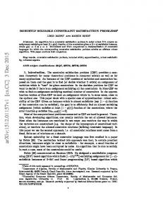
In order to see better the way that SBDS works, we will consider an example based on the 8-queens problem (Fig. 1). It is easy to see, that for any solution, we can find symmetrically equivalent solutions, by rotating the one found by 180◦ . In other words, for any solution to the problem, the assignment that places the queens in the position that results by a 180◦ rotation of the solution found, also forms a (possibly different) solution to the problem. We use the variable Qi to model the column that the queen at the i-th row is positioned at. Suppose that during search, the first two assignments made are Q 1 = 2 (denoted in Fig. 1 by X) and Q2 = 4 (marked in Fig. 1 by Y ). By S180 we denote the symmetry formed by the 180◦ rotation of the variable assignment. The symmetric assignments of Q1 = 2 and Q2 = 4, according to S180 , are Q8 = 7 (denoted in Fig. 1 by X 0 ) and Q7 = 5 (denoted in Fig. 1 by Y 0 ) respectively. 1 1 2
2
3
4
5
6
7
8
X Y
3 4 5 6
Y’
7
X’
8
Fig. 1. An example of symmetries in the 8-queens problem.
After having explored the part of the search tree that corresponds to those assignments, and backtracking from the decision Q2 = 4, we proceed to exploring the case Q1 = 2 and Q2 6= 4. If at some point we use the assignment Q8 = 7, then by also setting Q7 = 5, then we would only find nodes that correspond to nodes that are symmetric according to S180 and thus they have already been found in the branch of the search tree that dealt with the case Q1 = 2 and Q2 = 4. If on the other hand, it is Q8 6= 7, then we know that any solution we might come up with, will not be symmetric (with respect to S 180 ) to any solution found in the 2
case Q1 = 2 and Q2 = 4. Thus, the constraint that we should use is: Q1 = 2 ∧ Q2 6= 4 ∧ Q8 = 7 ⇒ Q7 6= 5 The above constraint only takes effect if at the same time it is set Q 1 = 2 and Q2 6= 4, i.e., when still at the subtree that corresponds to Q1 = 2 and while backtracking from the decision Q2 = 4, and at the same time Q8 = 7, which means, that if also Q7 = 5 then we can only end up with solutions symmetric to the ones already found. Thus we need to exclude such an assignment from taking place.
3
First Method
The first method that we deal with is the one described in [1]. In order to describe the way that the method works, we should first consider the search tree of a CSP and define some notation about it. Let CPr be a fixed set of constraints that model the CSP to be solved, and let P (·) denote the effect of propagation. Normally, the root of the search tree would be labeled by P (C Pr ). For any node of the search tree, such that Cstore is the constraint store at that node, and the node branches over some constraint c, the left and right child would have the constraint store P (CPr ∧ c) and P (CPr ∧ ¬c) respectively. In order to use the method described here, we assign a triple to each node as its label. More precisely, the root node is labeled by (∅, ∅, P (CPr )), while for any node labeled by (Cp , Cn , Cstore ) that branches over l the constraint c, the left child will be labeled by (C p ∧ c, Cn , Cstore ) while the right child will be labeled by r l r (Cp , Cn ∧ ¬c, Cstore ) (see Fig. 2). Moreover, it is Cstore |= Cstore ∧ c and Cstore |= Cstore ∧ ¬c. (C p, C n, C store ) c
c
(C p
l
( C p, C n
c, C n, C store )
r
c , C store )
Fig. 2. Model of search tree for the first method.
From the above we can see that “the positive” constraints are separated from the “negative” ones. The reason for this is the following: When the constraint c is being added, we know how search tree proceeds to explore the search space. The same holds also for the branch that uses the negation of the constraint, i.e. ¬c, but in this case, we also know that we have already found the solutions that correspond to that branch of the tree that the constraint c appears in its positive form, and thus the constraint should also be considered for symmetry breaking. l l Moreover, the reason we use Cstore |= Cstore ∧ c instead of Cstore = Cstore ∧ c (and the respective one for the right child), is that we want to model the fact that the constraint store at that point, except for Cstore ∧ c may also contain additional constraints (which will be exactly those that will perform the symmetry exclusion), while of course they should not violate C store ∧ c as needed. We denote by kck the set of solutions that satisfy the constraint c (and of course respect the domains of the variables), and let X be the set of all possible solutions to the problem. Moreover, let s be any symmetry of the given CSP. Here we consider symmetries as functions that on input of any constrain c, they return the constraint that is symmetric to c. Also, by s∗ : X → X , we denote a function such that for any set of solutions x ∈ X , s∗ (x) is a set that contains all the solutions are symmetric, according to s, to the elements of x. We will assume that for any constraint c, there is a constraint c 0 , such that s∗ (kck) = kc0 k, i.e, the symmetric of the solutions that satisfy c, are exactly the solutions that satisfy c 0 . Since there may be more than one constraints c0 with the above property, we will fix a function scon on constraints that we will assume it returns always a specific constraint such that s ∗ (kck) = kscon (c)k (so that instead of using any 3
one of all the possible constraints that have the exact same solutions as s ∗ (kck), we can uniquely refer to scon (c)). Now, let v be any internal node of the search tree, and let S be the set of all the symmetries we consider in the problem. We define the following constraint: E v (¬c) =
^
s∈S
scon (Cp ) → ¬scon (c
E v (¬c) is exactly the constraint that performs the symmetry exclusion. For all the symmetries in S, if the search tree is at a point that the constraints that are symmetric to the constraints modeled in previously searched nodes hold, then we want to exclude any nodes that also set true the symmetric of c, since, this case has already been explored by the left brother of v, and thus all solutions that would be found, when scon (c) holds, will be equivalent, according to some symmetry s ∈ S, to a previously found solution. Also, if that branch failed in the left brother, so it will in this case as well, and thus again it does not need to be considered. The method will set: l Cstore = Cstore ∧ c r Cstore = Cstore ∧ ¬c ∧ E v (¬c) It can be proved that the search trees defined as above, only find one solution for each set of symmetrically equivalent ones. Moreover, if S is the set of symmetries that are explicitly defined, the above search tree will also find one solution out of all the symmetrically equivalent ones, when the symmetries considered are the closure of S under composition and inversion. Thus, not only the symmetries defined explicitly will be used, but also the ones that are formed by repeatedly applying composition to the explicitly defined ones. The authors of [1] have used the constraint programming language Oz to implement the above search trees. The pseudo code for this method is given in Table 4.4.
4
Second Method
The method of Gent et al. makes use group theory to model symmetries. Thus first, we describe some basic group theory notions which are necessary to describe the method. 4.1
Group Theory Background
We define a group as a tuple hS, ◦, ei, where S is a set, ◦ is a closed binary operation over S and e ∈ S is the identity element, such that the following three conditions hold: 1. ∀a, b, c ∈ S it is (a ◦ b) ◦ c = a ◦ (b ◦ c), i.e. associativity holds. 2. ∀a ∈ S, a ◦ e = e ◦ a = a. 3. ∀a ∈ S, ∃a−1 , such that a ◦ a−1 = a−1 ◦ a = e, i.e, for each element, there exists the inverse of it, which also belongs to S. hT, ◦, ei is a subgroup of hT, ◦, ei, if T ⊆ S and T is a group under ◦, which means that T must also be closed under the operation ◦. As it will be seen later, subgroups are very important in describing symmetries. Now, the symmetric group SN is defined as SN ≡ hSΩ , ◦, ()i, where : – Ω is an ordered list of N elements, – SΩ is the set of bijective mappings Ω → Ω, i.e, each element of S Ω is a permutation of the elements of Ω, – ◦ is the composition function on elements of SΩ , – () is the identity mapping, i.e. the permutation that leaves the order of the elements of Ω unchanged. 4
In other words, SN is the group of all permutations of the N symbols of Ω. Since the number of permutations of N elements is equal to N !, the number of elements of S N is also N !. Given a subgroup G of SN , i.e. a group of certain permutations of N elements {1, 2, ..., N }, we define the following: – The orbit under G of i ∈ {1, 2, ..., N }, as Oi (G) = {g(i)|g ∈ G}. – The stabiliser of i ∈ {1, 2, ..., N } in G as StabG (i) = {g ∈ G|g(i) = i}. The orbit of an element represents all the possible positions that the element can be sent, using the permutations contained in G, while the stabiliser of the element is the set of all the possible permutations of G that leave the position of the element unchanged. An equivalence relation R on a set X, is a subset of X × X if it satisfies certain properties. Denoting by aRb that (a, b) ∈ X × X is an element of R, the properties that R must satisfy are: – aRa, ∀a ∈ X – aRb ⇒ bRa, ∀a, b ∈ X – aRb and bRc ⇒ aRc, ∀a, b, c ∈ X Now, for any group G with subgroup H, we can define an equivalence relation ∼, as: a ∼ b iff b ◦ a−1 ∈ H ∼ is an equivalence relation since all the above properties hold. The right cosets of H in G are the equivalence classes formed by using the above relation. A subset T of elements of G is called a right transversal of H if it contains exactly one element of each right coset of H. For instance, if we consider S4 , the symmetric group that contains the 24 permutations of the elements {1, 2, 3, 4}, we get the following right cosets of Stab S4 (1): c1 c2 c3 c4
= {[1, 2, 3, 4], [1, 2, 4, 3], [1, 3, 2, 4], [1, 3, 4, 2], [1, 4, 2, 3], [1, 4, 3, 2]} = Stab S4 = {[2, 1, 3, 4], [2, 1, 4, 3], [2, 3, 1, 4], [2, 3, 4, 1], [2, 4, 1, 3], [2, 4, 3, 1]} = {[3, 2, 1, 4], [3, 2, 4, 1], [3, 1, 2, 4], [3, 1, 4, 2], [3, 4, 2, 1], [3, 4, 1, 2]} = {[4, 2, 3, 1], [4, 2, 1, 3], [4, 3, 2, 1], [4, 3, 1, 2], [4, 1, 2, 3], [4, 1, 3, 2]}
For instance, we can see that the inverse of [2, 3, 4, 1] is [4, 1, 2, 3], whose composition with any element of c2 , results in a permutation that leaves the first element in the same position, and thus, the composition of the inverse of [2, 3, 4, 1] with any element of c2 belongs to StabS4 . A chain of stabilisers is computed by starting from a the stabiliser of a point as the first element of the chain, continuing with the stabiliser within the first element of another point, and so on. For instance, again for the case of S4 ,and starting arbitrarily with with point 1, we have: StabS4 (1) = {[1, 2, 3, 4], [1, 2, 4, 3, ], [1, 3, 2, 4], [1, 3, 4, 2], [1, 4, 2, 3], [1, 4, 3, 2]} StabStabS4 (1) (2) = {[1, 2, 3, 4], [1, 2, 4, 3]} StabStabStabS (1) (2) (3) = {[1, 2, 3, 4]} 4
Using the fact that the order of a subgroup must divide the order of the original group, we know that the order of each element of a stabiliser chain must divide the order of the previous stabiliser, and thus, usually, chains of stabilisers collapse soon to a subgroup that consists of only the identity element. 4.2
CSP Symmetries as Subgroups
Considering a given CSP, we will consider that the N elements of Ω = {1, 2, ..., N } represent either a CSP variable, a value or a variable/value pair. Then S N represents all the symmetries that might be applicable to the given CSP. Nevertheless, a CSP does not have to contain all the N ! symmetries described by S N , but only a subset of them. Moreover, even if the problem does contain all of them, since their number is very large, we might want to restrict ourselves to only some of them. 5
1
2
3
4
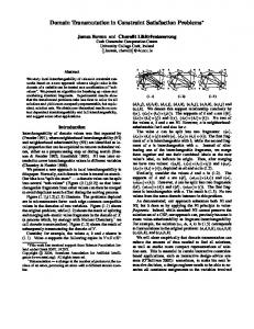
Fig. 3. Numbering of a 2 × 2 square.
Thus, what is needed is to select only certain elements of S N , such that they describe the desired symmetries of the CSP. This means, that in order to model the symmetries, we wish to find a certain set of permutations that generate that subgroup of SN which correctly represents the symmetries of the CSP. In order to construct the subgroup, we need to select a small number of permutations, and find all the permutations formed by using composition on them, so as to construct a closed subset of S Ω . As an example, consider the symmetries of the 2 × 2 square, with the cells numbered as shown in Fig. 3. The symmetries of the square can all be produced by using the subgroup of S 4 (i.e., the group of all 24 permutations of 4 elements) that is generated by only two permutations, namely p 1 = [3, 1, 4, 2] which models a rotation by 90◦ , and p2 = [3, 4, 1, 2] which models a horizontal flip. The composition of the above two results in the following permutations: p1 ◦ p1 = [4, 3, 2, 1], rotation by 180◦ . p1 ◦ p1 ◦ p1 = [2, 4, 1, 3], rotation by 270◦ . p1 ◦ p1 ◦ p1 ◦ p1 = [1, 2, 3, 4], rotation by 360◦ , which is also the identity mapping. p2 ◦ p1 = [4, 2, 3, 1], rotate by 90◦ and then flip horizontally. p1 ◦ p2 = [1, 3, 2, 4], flip horizontally and then rotate by 90 ◦ . p1 ◦ p1 ◦ p2 = [2, 1, 4, 3], flip vertically. Any other way of using the composition will not result in a new element, and thus the above form a subgroup of S4 . We can see that this subgroup contains only 8 elements, instead of 24 = 4! which is the number of elements of S4 . The subgroup generated is known as D4 , the dihedral group with 8 elements. In this example, it is easy to see that O3 (D4 ) = {1, 2, 3, 4}, since element 3 is moved to position: – – – –
4, 1, 2, 3,
by by by by
p1 , p2 , p1 ◦ p1 , and p1 ◦ p1 ◦ p1 ◦ p1 , the identity.
Also, StabD4 (3) = {p1 ◦ p1 ◦ p1 ◦ p1 , p2 ◦ p1 }, since these are the only two permutations that leave point 3 in the same position.
4.3
SBDS using group theory
The implementation of the second method is based on combining two systems. More precisely, given a CSP, the Constraint Logic Programming system ECLi PSe performs the tree search needed to solve the CSP using symmetries, while the computational group theory system GAP (Groups, Algorithms and Programming) is being used in order to handle symmetries as groups, providing all the theoretical tools needed, like the symmetry group, the stabilisers and so on. ECLi PSe can this way use all the necessary elements of group theory, without having to explicitly implement them. While testing a particular partial assignment A, and after having explored the part of the search tree that corresponds also to the assignment V ar = V al, SBDS will post for each element g of the symmetry group, the additional constraint g(A) ⇒ g(V ar 6= V al). Thus, whenever we come up with some symmetric assignment of A, the symmetric equivalent of V ar = V al will not be considered. This also resemblances the way that the first method performs SBDS. 6
4.4
Implementation
Many CSPs contain a very large number of symmetries, making it impractical to model explicitly all of them. An example of such a case is a 7 × 7 matrix with full symmetry on rows and columns, i.e., a solution matrix is equivalent to any other that is the result of swapping any number of rows and/or columns of the matrix. There are 7! possible permutations of the rows and 7! possible permutations of the columns, resulting in a total of 7! × 7! = 25, 401, 600 symmetries. Instead, only a few symmetries are explicitly modeled, and GAP is used to generate the corresponding symmetry group. The main idea of the algorithm, which is shown in Table 4.4 is that at any point of the search, when exploring the branch that corresponds to a given partial assignment A, and while backtracking from the the decision V ar = V al, for some variable V ar that was not assigned to a value in A so far, and some value V al that belongs to its domain, in order to avoid visiting all symmetric equivalent assignments of A ∧ V ar 6= V al, the additional constraint g(A) ⇒ g(V ar 6= V al) is posed for all symmetries that can be applied. By using GAP so as to handle symmetries as subgroups, this is done in systematic manner, using chains of stabilisers. The algorithm is described more formally below. – A is the current partial assignment that has assigned values to certain variables. – Stab is the last member of the stabiliser chain computed until the last assignment and thus describes the subgroup of G that stabilises all the SBDS points that are assigned to a value, using the current assignment. – RT chain = hRT1 , RT2 , ..., RTk i is a sequence of right transversals that correspond to the assignments made so far, where RTi , is a set that contains a representative group element for each coset of Stab i in Stabi−1 . Then g ∈ RT chain is any group element such that it is g = p k ◦ pk−1 ◦ ... ◦ p1 , where pi ∈ RTi . In other words, RT chain is a compact way of modeling all partial assignments that are symmetric to A, since, all these assignments can be expressed by some g ∈ RT chain. In each step, given Stab, A, RT chain, a variable-value pair is chosen and GAP will compute the next element of the stabiliser chain (by finding the stabilisers of the new point in the last element of the chain), as well as the right transversal of the (new) last element of the chain in the previous one, so that RT chain can be updated. RT chain, as also mentioned before, models the current set of all the symmetries that could be applied to the current partial assignment Now, if the assignment V ar = V al results in finding a solution, then the final assignment is a solution to the CSP, which is not symmetric to any other solution that wes previously found. If on the other hand, the assignment results in a failure, backtracking is performed and the additional constraint g(A) ⇒ g(V ar 6= V al) must be posed, for all symmetries described by RT chain. Instead of repeatedly applying the above constraint for all the suitable symmetries, we note that it only has to be posed for these symmetries g of the current chain for which the symmetric equivalent of the assignment A, i.e. g(A) is true, and thus we do not need to do anything for those that G(A) is false.
5
Examples
The two methods were applied in a variety of CSPs, showing a great impact on reducing the number of solutions found (and thus reducing the size of the search tree) when SBDS was used. Unfortunately, there was not an example common in both of them, which could help us in making a comparison between the way that the two techniques behave. 5.1
Example for the First Method
Here we consider the problem of Graph Coloring, according to which, given a graph G = (V, E) and a set of colors, we wish to color all the nodes of the graph in a way that if (u, v) ∈ E, then u and v should not have the same color. If such a coloring exists, then we also want to find the smallest subset of colors that can still provide a solution to the problem. As a symmetry here, we consider permutations of colors, i.e, two colorings are symmetric, if the first can result from the second, by permuting the colors. In order to model the symmetries, only the transposition of 7
Table 1. Pseudocodes for both methods Method 1 - Backofen et al. procedure ses(Cp , Cstore ) if Cstore determines solution a then write a elsif ⊥ ∈ / Cstore then choose a constraint c l Cstore := Cstore ∧ c Cpl := Cp ∧ c ses(Cpl , Cstore ) r Cstore := Cstore ∧ ¬c ∧∀s ∈ S : scon (Cp ) → scon (¬c) r ses(Cp , Cstore ) endif
Method 2 - Gent et al. sbds search:= proc(Stab, A, RT chain) local P oint, N ewStab, RT, N ewA, BrokenSymms, g; choose(V ar, V al); P oint:=var value to point(V ar, V al); N ewStab:=Stabilizer(Stab, P oint); RT :=RightTransversal(Stab, N ewStab); N ewRT chain:=RT chain∧ RT ; assert(V ar = V al); if sbds search(N ewStab, A ∧ V ar = V al, N ewRT chain) = true then return true; else retract(V ar = V al); BrokenSymms:= lazy check(N ewRT chain, A); for g ∈ BrokenSymms do assert(g(A) ⇒ g(V ar 6= V al)); end do; return sbds search(Stab, A, RT chain); end if end proc
any two elements is given explicitly. Any possible permutation of colors can be formed by repeatedly using transpositions of two colors, while the method excludes also the composition of all the symmetries that are explicitly given. Table 2. Number of solutions for the graph coloring problem, using the first method. Vertices 20 25 30 35
Edges Colors Without SBDS With SBDS 114 6 162 24 185 8 52,733 61 292 9 551,022 97 339 9 3,428,853 168
In Table 5.1, we can see the number of solutions found, with and without using symmetry breaking during search. From the table it can clearly be seen that the use of symmetry breaking has resulted in a significant decrease of the number of different solutions found. 5.2
Example for the Second Method
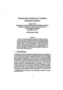
Using the problem of Coloring Dedecahedra we can easily see the impact of applying SBDS using the method of Gent et al. The Dodecahedron is a regular polyhedron that has 12 pentagonal faces, 20 vertices and 30 edges, as depicted in Fig 4. Again, we want to color the vertices, so that no two vertices connected by an edge share the same color, given a set of m colors. It can be shown that the symmetry group of dodecahedron is isomorphic to the group of even permutations of five objects. This group is denoted by A5 and it contains 60 elements. Again, as in the previous case, any two permutations of the m colors result in a symmetrically equivalent solution. Thusm the total number of symmetries, resulting either from the properties of the dodecahedron, or the permutations of colors, is equal to 60 × m!. 8
Fig. 4. Dodecahedron.
The symmetry group is constructed in GAP using only the following four generators: – – – –
rotation of the vertices about a face, rotation about a vertex, swapping the first two color indices, cycling the color indices by one place.
We can see that the first two generators correspond to symmetries caused by the structure of the dodecahedron, while the other two correspond to symmetries caused by the color permutations. The group formed by the above generators, models all of the 60 × m! symmetries contained in the problem formulation. The results, for two values of m, with and without the use of symmetry breaking is shown in Table 5.2. Again, the decrease of the search space is rather impressive. (When only ECL i PSe is used, SBDS is not applied in solving the problem.) Table 3. Number of solutions for the dodecahedron coloring problem, using the second method. m Symmetries ECLi PSe Solutions GAP- ECLi PSe Solutions 3 360 7200 31 4 1440 1.7 × 10⁸ 117902
6
Comparison of the two methods - Conclusions
Both methods described here deal with symmetry breaking during search. The main idea in both of them is essentially the same: when the search method backtracks from a decision, it uses additional constraints to make sure that the symmetric equivalents of the failed (partial) assignments tested will not be considered in the future. This leads to efficient pruning of the search tree. By using the knowledge acquainted by the so far searching, the methods avoid to make assignments that are known to fail, or lead to solutions that could be found just by applying a certain set of symmetries to some previously encountered solution. Nevertheless, as it seems, symmetry breaking the way presented, does not really need to explore a branch before pruning other symmetric branches. This means, that we do not have to finish exploring a branch, so as either to find all solutions that can lie within the branch, or realize that the branch leads to a failure, before putting symmetry breaking into effect. Symmetry breaking works by utilizing the knowledge of the partial assignments made, in order to reach a node, not the results from searching. Whenever we reach a node that we know that it has a symmetric equivalent that has been or will be explored, we do not need to proceed to its subtree. Any information that we would gain by doing it, can be acquired by searching the symmetric node, or looking at the results of searching down that tree, if the search has already been performed. Thus, given a set A of nodes in the search tree that are all symmetrically equivalent with each other, we only need to know that exactly one of them will be fully explored. All others can be skipped, regardless of whether we have explored one fully so far or not. 9
This fact makes SBDS suitable for parallel implementation as well. Different branches can be assigned to different machines, specifying that out of all sets A of symmetrically equivalent nodes, only the subtree of the leftmost will be explored. Any machine that reaches a point that corresponds to a node contained in A, will not proceed to explore its subtree, unless it is the leftmost branch. Moreover, the two techniques seem to be rather similar. Below, we can see the two parts of the pseudocode for each technique, that actually perform the symmetry breaking. Backofen et al. Gent et.al for g ∈ BrokenSymms do ∧∀s ∈ S : scon (Cp ) → scon (¬c) assert(g(A) ⇒ g(V ar 6= V al)); end do; The two pieces of code appear to pose the the same constraint, only described in a different context: after having explored the left subtree of a node (the one that deals with c in the first method and the one that had posed V ar = V al in the second), and before proceeding to the right, an additional constrained is posed, that aims at avoiding to visit the symmetric equivalent of the left subtree (i.e s con (Cp ) → scon (¬c) for the first one and g(A) ⇒ g(V ar 6= V al) for the second). In both cases, the constraint asserts that if the symmetric equivalent assignment formed by the path from the root to the father of the two subtrees appears again, then the corresponding symmetric of the last assignment that was dealt with in the left subtree should not be considered. By looking at the description of the two methods, we can see that the method of Gent et al. can be described in a more elegant manner. With the use of the background supplied by group theory, the generation of a large number of symmetries by only providing explicitly a small subset of them, is much more compact. On the contrary, Backofen et al. in order to use their method first prove how the method works by explicitly providing all symmetries, and then they try to generalize this to the closure of symmetries. Even from the programmer’s point of view, Backofen et al. need to implement everything from scratch, while Gent et al. by making use of ECLi PSe and GAP, provide a method much easier to implement. By using GAP, symmetries are easily handled as subgroups, providing a more compact way to write a CSP solver, without the need to deal with the group-theoretic implementation details. Nevertheless, even though the main idea is the same, it has not yet been proven whether the two methods are actually equivalent or not. It seems that Gent et al. provided a refinement of the method of Backofen et al., even though there is no formal proof of it.
References 1. Backofen, R., Will, S., Excluding symmetries in constraint-based search. Constraints 2002 7(3) 2. Gent, I., Harvey, W., Kelsey, T., Groups and Constraints: Symmetry breaking during search. CP 2002, LNCS 2470, p.p. 415-430 3. Gent, I., Smith, B., Symmetry Breaking During Search in Constraint Programming. Proceedings of ECAI-2000 (W.Horn, ed.), IOS Press, 2000, p.p 599-603
10