ENOC-2008, Saint Petersburg, Russia, June, 30–July, 4 2008
SYNCHRONIZATION OF LOCAL OSCILLATORS IN THE LATTICE LOTKA–VOLTERRA MODEL DUE TO LONG RANGE MIXING.
Anton Efimov
Alexey Shabunin
Department of Radiophysics and Nonlinear Dynamics Saratov State University Russia
[email protected]
Department of Radiophysics and Nonlinear Dynamics Saratov State University Russia
[email protected]
Abstract We study a simple stochastic cellular model of Lattice Lotka–Volterra class driven by particular external forces. To simulate the system dynamics we perform Kinetic Monte Carlo simulation. We demonstrate the spatial synchronization phenomenon of local oscillators and a global oscillations appearance (the Hopf bifurcation). The extent of the external influence was chosen as a control parameter of the system. Key words Nonlinear systems, stochastic systems, synchronization, bifurcations, discontinuous systems, selforganization. 1 Introduction Although Lotka’s and Volterra’s pioneering works devoted to competitive behavior in chemical and population dynamics was published in first half of the 20th century the problems of competitive dynamics are still actual and full of interest for many scientists. Synchronization effects, spatiotemporal oscillations and fluctuations, pattern formation and fractal features – here is not a full list of phenomena a scientist deals with when studying Lotka–Volterra systems [1]-[15]. In addition these effects are extremely widespread in experiments and real systems (especially in catalytic chemistry and biology [16]-[22]). There are two basic types of models designed for Lotka–Volterra systems simulation. The first one is a group of phenomenological macroscopic models based on the ODE description (for example mean-field (MF) models). Most of them predict a neutral stability of the systems under consideration i.e. the system solution is an infinite number of closed trajectories around the center. Unfortunately such a forecast is often unrelated to the data observed in nature. As a rule in a real life the system selects some preferred regime depending on ad-
ditional parameters (for example noise character, spatial parameters and etc.) and it is robust to the initial conditions variations. Usually the models above ignore the system spatial dynamics, while the spatial effects are responsible for the variety of nontrivial phenomena observed. The second type of the models based on various stochastic cellular automata and other numerical methods provide the direct microscopic simulation of the underlying processes. The Kinetic Monte Carlo (KMC) simulation is one of them. This is a kind of probabilistic cellular automaton suitable in our investigations. This method enables to consider all aspects of spatial and temporal dynamics of the system, but requires a long computer calculation. The last fact limits the size of simulated system. In earlier studies [8]-[10] the cyclic Lattice Lotka– Volterra (LLV) models were considered. These models describe a variety of heterogeneous autocatalytic processes taking place on an underlying substrate or a closed chain of predator–prey interactions in population dynamics context (also taking place on a substrate). The special features of these models are restricted geometry of the support, local character of interactions and diffusion absence. Both (2+1)-LLV ((LLV from here) and (4+1)-LLV systems were studied in [8]-[10] and in both cases the systems were subjected to the MF description and KMC simulation. In the current study we consider LLV system under specific external influence we call “external mixing”. At first we outline the results of previous investigations essential for our considerations. Then we introduce long range mixing and describe how even a weak external mixing bring the system from local oscillatory behavior to limit cycle robust oscillations. Moreover we try to find out the role of spatial patterns in LLV model dynamics and discuss the possibilities of system controlling.
2 The LLV system and its MF description Let’s consider a square regular lattice containing N = L × L sites. Every site is a three-state unit governed by its neighborhood state and undergoing a series of cyclic transformations with corresponding transition rates. The site states are denoted by X, Y and S symbols while the transition rates by k1 , k2 , k3 . A chosen unit undergoes the transition with some probability, if one site in its close vicinity has an appropriate phase. Thus we have the LLV transition scheme of the following form [8]: k
X + Y →1 2Y, k2
(1)
Y + S → 2S, k3
S + X → 2X, It means that randomly chosen X-unit turns to Y -state with probability k1 if a randomly chosen neighbor is Y . The same is for the rest lines of scheme. System (1) belongs to Lattice Lotka–Volterra class. This model is very simple, but it enables to study nontrivial effects resulting from the locality of interactions and nonlinearity. From the dynamical point of view such a system may be described by the mean field rate equations. Today it’s well known that MF prediction for this system type differ sufficiently from the observed data because of the spatial restrictions of the support. But MF approach is still useful. Taking it into account provides with some general information we can use for further considerations. The MF dynamics for the LLV system has been described in details in [8]. Here we just briefly remind the main results needed below. The MF equations associated with scheme (1) are:
x˙ = −k1 xy + k3 x(1 − x − y) y˙ = k1 xy − k2 y(1 − x − y)
(2)
where x and y are the relative concentrations of the corresponding sites and k1,2,3 – are the kinetic constants respectively. It is reasonable to focus on a region within the following boundaries: x = 0, y = 0, x + y = 1. The considered variables have a physical meaning in that case. The system (2) has four equilibrium points: three saddle³points P1 (0; 0), P2 (1;´ 0), P3 (0; 1), and a center P4 k1 +kk22 +k3 ; k1 +kk32 +k3 . The model is known to demonstrate conservative periodic oscillations and the phase portrait of the system consists of an infinite number of closed trajectories around the center P4 . The linearized frequency associated with the small oscillations around the center [8] is found to be: µ ω=
k1 k2 k3 k1 + k2 + k3
¶1/2 (3)
The corresponding amplitudes depend on the initial conditions. Changing the parameters ki results in time scale and orbits shape modifications. However, the system is insensitive to parameters variations in terms of bifurcational analysis. 3 Kinetic Monte Carlo simulation Since the homogeneous mean-field model is not appropriate to describe the full variety of phenomena arising from the support spatial restrictions, we perform the Kinetic Monte Carlo (KMC) simulation of unit’s behavior. This is an alternative tool for initial scheme investigation. It’s based on the microscopic simulation of the lattice processes. The KMC simulation algorithm is as follows: 1. A lattice unit and its neighbor unit random selection at every microscopic step. 2. Units state checking and making a comparison with the initial scheme conditions. 3. As soon as comparison has been passed successfully, the corresponding transformation is realized with probability ki /max (k1 , k2 , k3 ). 4. The end of microscopic step. Return to item 1. Every algorithm time unit called Monte Carlo step (MCS) contains N microscopic steps. To describe the system dynamics it is reasonable to use x and y variables which represent averaged relative concentrations of units. These variables define system state ambiguously (their values are independent of the units distribution in space). But they easily define the lattice state in general. According to previous investigations the time evolution of the system contains two intervals – a transient process and stochastic oscillations around fixed point P4 . The oscillations tend to zero at the limit of infinite lattice size. Starting from the different initial conditions a phase trajectory is attracted by the locality of the point P4 . It looks like P4 is a stable focus and it attracts all trajectories started throughout its basin. It is interesting that when simulated by KMC the model demonstrates dissipative dynamics at global level. It well known from the previous investigations [8], [10] in case of random and uniform initialization spontaneous clusters formation takes place on the surface. And this process is known to be responsible for transient behavior. The units forming a single cluster have the same phases. Since unit’s interactions have local character the neighboring clusters interact only via their boundaries. Some of them increase their size in expense of others and as long as the lattice is far from poisoning (one state absolute domination) the clusters boundaries demonstrate a continuous motion. Furthermore the homogeneously initialized lattice consists of domains after the clusters formation. The domains are local oscillators demonstrating out of phase nonperiodic oscillatory behavior. The oscillators scale correlate with the mean cluster size. As it is known these oscillators have fractal structure [9].
KMC simulation of the system with long range mixing Returning to the initial scheme (1) we assume now the presence of an external force providing a possibility of immediate phase exchange between lattice units. Moreover we stipulate the probability of such event to be independent of the unit position. In other words we activate an external mixing influence providing a “shuffling” effect on the surface. Such an innovation of the initial system seems to be baseless. But it is not so. The “shuffling” external influences are not exotic for systems under consideration. In the case of population dynamics such a mixing may be realized by the natural migration processes or by the artificial transport activity. If we deal with autocatalytic reactions on the surface, some transport agent that is not involved in reactions may be responsible for “shuffling”. These processes are also called ”long range diffusion”. Consider the simulation algorithm and introduce some quantitative characteristic for mixing intensity definition. As long as the above mentioned influence does not affect the interaction rules, we perform the same simulation algorithm as in previous chapter 1. The only modification here is the “shuffling” steps added at every MCS. At every “shuffling” step two random lattice sites are chosen. Then the chosen units exchange their phases. The number of “shuffling” steps corresponds to the mixing extent. To characterize the mixing degree we use the following parameter:
1.2 p=0 p=0.03
1.0 0.8
x
As it was pointed above the stochastic oscillations look like a small fluctuations around the fixed point P4 if the lattice is large enough. Their intensity decreases with the lattice size growing just as in ensembles of non-interacting oscillators. But oscillations stay robust in small parts of the lattice. The dynamics of the system is then a superposition of local asynchronous oscillations. That is why increasing the lattice size, one observes global oscillations suppression. Notice that KMC-behavior differs sufficiently from the MF approach. Instead of conservative periodic MFbehavior the irregular oscillations vanish when the lattice size increases. The decrease of the autocorrelation function and the widespread power spectrum for KMCoscillations (not shown) are the evidence of the irregular oscillating process taken place on the surface. Variation of the parameters k1 , k2 , k3 doesn’t induce any qualitative changes in the system behavior, which remains in agreement with the mean-field theory.
0.6 0.4 0.2 0 0
200
400
600
800
1000
t, MCS
Figure 1. Time realizations of the X -units global concentrations starting from the same initial conditions x0 = y0 = 0.33 for p = 0 (mixing absence) and p = 0.03. Parameters of the system are: k1
= k2 = k3 = 1, L = 2048 sites.
4
p=
³n´ N
,
(4)
where n is number of “shuffling” steps at every MCS and N is a total number of lattice sites. As the “shuffling” keeps the total number of X, Y and S-sites unchanged, mixing implementation itself does not effect on current state of the system in terms of
global concentrations of the units. But mixing causes dramatic changes in the system dynamics by changing the local space configurations of the states distribution. Figure 1 represents a comparison of two different KMC realizations of scheme (1) for p = 0 and p = 0.03. The observed stochastic oscillations have been described for the case of mixing absence (p = 0). These oscillations have low intensity if the lattice is large enough and look like small fluctuations of the global concentrations around the fixed point P4 . Global oscillations are starting with the same initial conditions and the same parameters values but with mixing extent p = 0.03 (the black line on the fig. 1). According to our expectations the oscillations characteristics have approached the ones observed at MF level. These oscillations appear at the global level and their regularity is much bigger. The shape of the phase orbits changes with parameters ki variation just as in the case of the mean-field prediction. Furthermore, the dependence of oscillations frequencies on parameters ki looks like the corresponding function graph for expression (3), but the regime remains robust in a wide range of initial conditions. Starting from different initial points in phase space a phase trajectory comes to the attracting set after the transient process. It is possible to define this attractor as a noisy limit cycle by analogue with the deterministic systems. Though the noise is an essential part of our model, we suppose that these stochastic oscillations tend to take a regular form with the lattice size growing because of better statistics. To verify this hypothesis we have considered two power spectra for different lattice sizes L = 256 sites and L = 512 sites (see fig. 2). The other parameters of the system were identical for both spectra. The characteristic peaks of the spectra have multiple frequencies. Moreover, despite the fact that the lattice linear sizes ratio does not exceed the value
0
1 p=0 p=0.01 p=0.02
−10
−20
y
Power spectrum (dB)
L=512 L=256
0.5
−30
−40 0.00
0.05
0.10
0.15
0.20
0.25
Frequency (MCS −1)
Figure 2. Power spectra of the global oscillations of X concentrations for two different lattice sizes. Initial conditions and parameters are the same as in the fig. 1. Mixing extent is p = 0.02.
0.5 x
1
Figure 4. The phase portraits for different values of the mixing extent p. Parameters of the system are: k1 = k2 = k3 = 1,
L = 1024 sites. Initial conditions were fixed at values x0 = y0 = 0.33 for all realizations. The transient processes have been truncated and only steady-state oscillations are shown. Lines with arrows represent the saddles manifolds.
0.15
0.10
σ
k1=1.0 k1=1.8 k1=3.0
0.05
0.00
0
0.01
0.02
0.03
0.04
p
Figure 3. Dispersions for the processes x(t) depending on the mixing extent p for different values of k1 . Lattice size is L = 500 sites. Initial conditions and others parameters are the same as in figure 1.
two, the noise backgrounds of the spectra differ sufficiently. Therefore at the limit of infinite lattice we will get periodic oscillations of state concentrations. Continuing to consider oscillations features let’s take a closer look to their amplitude. There is no difficulty in understanding why the mean amplitude of oscillations is insensitive to the lattice size changes. This corresponds to the definition of the mixing strength p which shows the part of the lattice subjected to the shuffling effect at every simulation time step. That’s why different lattices undergo the same shuffle effect for a fixed value of p. But the oscillation amplitudes and shapes are strongly determined by the value of p. To investigate the influence of the mixing parameter p we increase the mixing extent step-by-step starting from value p = 0 and we study the dispersion of the process as a function of p (see the graphs on the fig. 3). We also describe the phase space organization for different external influences (see fig. 4).
When the mixing strength is sufficiently small there are no observable changes of the system dynamics in comparison with the situation described in the section III. The dispersion value is close to zero and there is a noisy stable focus at point P4 . Increasing the value of p the focus loses its stability and at the critical moment the global oscillations appear. Now the point P4 seems to be an unstable focus. Further increase of the mixing degree results in monotonous linear growth of dispersion. It corresponds to oscillation amplitudes increase as a square root of the value of parameter p. All of these facts indicate that the global oscillations in the lattice emerge as a result of the analogue of the supercritical Hopf bifurcation at the presence of noise. If the mixing is strong enough, the phase trajectories are located in the close vicinity of the contour formed by manifolds of the saddles P1 , P2 , P3 (see fig. 4) and there is a high probability for their contingence because of noise perturbations. As a esult the corresponding species dies out and the oscillations are interrupted. Figure 3 demonstrates three bifurcation curves for different values of the parameter k1 . As is easy to see the bifurcational value pcr depends on the transition rates of the system. More precisely, it is defined by the imbalance degree of the parameters ki . The greater the difference of the parameters, the smaller bifurcation value pcr . Moreover, in this case the poisoning of the lattice occurs at the lower pcr value. Consider now the processes on the lattice giving rise to such a bifurcational behavior of the system. For this purpose let’s take a closer look at the system spatial dynamics. Figure 5 demonstrates a series of snapshots of the lattice in gray-scale. The homogeneously initialized lattice (fig. 5 (1)) without mixing (p = 0) turns to state fig. 5 (2) after 10000 MCS. This clustering state of the lattice has been described in section
Figure 5. A series of snapshots for the lattice (L = 256 sites) in gray-scale. Each of the states is marked by the corresponding gray tone. (1) homogeneously initialized lattice (t = 0M CS ), (2) - the lattice surface at the moment t = 10000M CS (p = 0), (3) - the lattice surface at the moment t = 10000M CS (mixing extent p = 0.02). Initial conditions are x0 = y0 = 0.333. The parameters are fixed in the values k1 = k2 = k3 = 1.
50 p=0.02 p=0.0
30
10
∆Φ
III. The same lattice turns to state fig. 5 (3) when the mixing (p = 0.02) is added. The last snapshot of the lattice differs sufficiently from the state (2). The clusters are not homogeneous now. They contain single units from other clusters relocated by the ”shuffling”. These units are the centers of future transformations within the clusters. As a result of mixing implementation the transformations occur not only at the cluster borders but throughout lattice. It is clear that relocated sites more often have the phase which dominates on the lattice at the moment. Therefore the lattice surface becomes colored with dominating tone almost uniformly and local oscillators demonstrate synchronous behavior. To demonstrate the synchronization effect obviously we consider the oscillations of local parts of the lattice with linear size l = 64 sites. Figure 6 demonstrates two dependences of phase differences for two local oscillators in case of mixing absence (p = 0) and p = 0.02. We introduce the phase of oscillator as follows:
−10
−30
−50
0
5000
10000
15000
20000
t, MCS
Figure 6. Phase differences for two local oscillators as a function of time depending on mixing presence. Parameters values are k1 = k2 = k3 = 1. Initial conditions are the same as in the fig. 1. Linear lattice size is L = 256 sites and the linear size of the local oscillators is l = 64 sites.
µ
¶ |y − yav | Φ = arctg , |x − xav |
(5)
where xav and yav are the coordinates of P4 . In the absence of the mixing the oscillations of different parts of the lattice are weakly correlated and their phase difference is not a constant in time. Increasing of the mixing extent provides phase synchronization of the local oscillators and their phase difference fluctuates near the value ∆Φ = 0. 5 Conclusions We considered the Lattice Lotka–Volterra model with long range diffusion by means of Kinetic Monte Carlo simulation. The system dynamics is strongly determines by the intensity of the mixing effect. Increase
of the mixing results in global oscillations appearance due to the supercritical Hopf bifurcation. The critical value of the mixing extent pcr depends on the imbalance of the parameters ki and insensitive to the lattice size. It is established that in the infinite lattice size oscillations have periodic form. Further increase of the p leads to the growth of oscillation amplitude and finally to the lattice poisoning. It was determined that phase synchronization of the local oscillators underlies such a behavior. Mixing implementation provides units exchange between the clusters and local oscillators and results in their synchronous dynamics. It may seem to be a trivial result that mixing leads to synchronization effect. But the mixing strength we have considered was not enough to create a homogeneous distribution of unit states over the lattice by itself. The obtained results ex-
planation is the partial destruction of the clusters. The processes of cluster formation serve as some regulating factor which determine the stability of the fixed point P4 . When mixing processes destroy the cluster structure the point P4 loses stability and the lattice becomes poisoned. If the value of p is not so big and clusters are still exist, the system demonstrates a periodic motion with corresponding amplitude. Such a result gives an opportunity of system controlling. We can obtain a regime required by means of implementation of different influences destructing the clusters with a greater or lesser extent.
References R.M. Ziff, E. Gulari and Y. Barshad “Kinetic phase transitions in irreversible surface-reaction model,” Physical Review Letters, no. 56, p. 2553, 1986. E.V. Albano “Monte Carlo simulations of surface chemical reactions:Irreversible phase transitions and oscillatory behaviour,” Computer Physics Communications, no. 121-122, p. 388, 1999. E.V. Albano and J. Marro “Monte Carlo study of the CO-poisoning dynamics in a model for the catalytic oxidation of CO,” Journal of Chemical Physics, no. 113, p. 10279, 2000. M. Tammaro and J.W. Evans “Chemical diffusivity and wave propagation in surface reactions: latticegas model mimicking CO-oxidation with high COmobility,” Journal of Chemical Physics, no. 108, p. 762, 1998. D.J. Liu and J.W. Evans “Symmetry-breaking and percolation transitions in a surface reaction model with superlattice ordering,” Physical Review Letters, no. 84, p. 955, 2000. Y. De Decker, F. Baras, N. Kruse and G. Nicolis “Modeling the NO + H2 reaction on a Pt field emitter tip: Mean-field analysis and Monte-Carlo simulations,” Journal of Chemical Physics, no. 117, p. 10244, 2002. V.P. Zhdanov “Surface restructuring and kinetic oscillations in heterogeneous catalytic reactions,” Physical Review E, no. 60, p. 7554, 1999. A. Provata, G. Nicolis and F. Baras “Ocillatory Dynamics in Low Dimensional Lattices: A Lattice Lotka-Volterra Model,” Journal of Chemical Physics, no. 110, p. 8361, 1999. G.A. Tsekouras and A. Provata “Fractal properties of the lattice Lotka-Volterra model,” Physical Review E, no. 65, p. 016204, 2002. A.V. Shabunin, A. Efimov, G.A. Tsekouras and A. Provata “Scalling, cluster dynamics and complex oscillations in a multispecies Lattice Lotka–Volterra Model,” Physica A, no. 347, pp. 117-136, 2005. R. Monetti, A. Rozenfeld, E. Albano “Study of interacting particle systems: The transition to the oscillatory behavior of a prey-predator model,” Physica A, no. 283, pp. 52–58, 2000. T. Antal, M. Droz, A. Lipowski and G. Odor “Critical
behavior of a lattice prey-predator model,” Physical Review E, no. 64, p. 036118, 2001. M. Droz and A. Pekalski “Different strategies of evolution in a predator-prey system,” Physica A, no. 298, pp. 545–552, 2001. J. E. Satulovsky and T. Tome “Spatial instabilities and local oscillations in a lattice gas Lotka–Volterra model ,” Journal Mathametical Biology, no. 35, pp. 344– 358, 1997. B. Spagnolo, M. Cirone, A. La Barbera and F. de Pasquale “Noise-induced effects in population dynamics,” Journal of Physics: Condensed Matter, no. 14, pp. 2247–2255, 2002. G. Ertl “Oscillatory kinetics and spatiotemporal selforganization in reactions at solid surfaces,” Science, no. 254, pp. 1750–1755, 1991. G. Ertl, P.R. Norton and J. Rustig “Kinetic oscillations in the platinum-catalyzed oxidation of CO,” Physical Review Letters, no. 49, pp. 177–180, 1982. C. Voss and N. Kruse “Chemical wave propagation and rate oscillations during the N O2 /H2 reaction over P t,” Ultramicroscopy, no. 73, pp. 211–216, 1998. G. Theraulaz, E. Bonabeau, S.C. Nicolis, R.V. Sole, V. Fourcassie, S. Blanco, R. Fournier, J.L. Jolly, P. Fernandez, A. Grimal, P. Dalle and J.L. Deneubourg “Spatial patterns in ant colonies,” Proceedings of National Academy of Sciences USA, v. 99, no. 15, pp. 9645–9649, 2002. E. Ben-Jacob, O. Shochet, A. TenenBaum, I. Cohen, A. Czirok and T. Vicsek “Generic modelling of cooperative growth patterns in bacterial colonies,” Nature, no. 368, pp. 46–49, 1994. J.L. Deneubourg, A. Lioni and C. Detrain “Dynamics of aggregation and emergence of cooperation,” Biological Bulletin, v. 202, no. 3, pp. 262–267, 2002. F. Saffre and J.L. Deneubourg “Swarming strategies for cooperative species,” Journal of Theoretical Biology, v. 214, no. 3, pp. 441–451, 2002.