Synergistic Techniques for Better Understanding and Classifying the ...

DOI: 10.1007/s00267-004-0058-1

Synergistic Techniques for Better Understanding and Classifying the Environmental Structure of Landscapes BRETT A. BRYAN* Policy and Economic Research Unit CSIRO Land and Water Private Bag 2, Glen Osmond South Australia 5064 Australia

ABSTRACT / The desire to capture natural regions in the landscape has been a goal of geographic and environmental classification and ecological land classification (ELC) for decades. Since the increased adoption of data-centric, multivariate, computational methods, the search for natural regions has become the search for the best classification that optimally trades off classification complexity for class homogeneity. In this study, three techniques are investigated for their ability to find the best classification of the physical environments of the Mt. Lofty Ranges in South Australia: AutoClass-C (a Bayesian classifier), a Kohonen Self-Organising Map neural network, and a k-means classifier with homogeneity analysis. AutoClass-C is specifically designed

Ecological land classification (ELC) is the process of defining and mapping homogeneous natural ecosystems and environments at a specific scale of analysis (Claessen and others 1994; Runhaar and Udo de Haes 1994; Sims and others 1996; Bailey 1996; Carter and others 1999; Omernik 2004) and has been a common tool of the geographer, ecologist, planner, and environmental manager for many years (Christian and Stewart 1968; Mabbutt 1968; Loveland and Merchant 2004). ELCs are usually based on biologically relevant physical environmental parameters but may also include some biological parameters such as vegetation type (Bailey 2004). ELCs have been conducted for many KEY WORDS: Landscape; GIS; Ecological land classification; Environmental gradients; Cluster; Multivariate analysis Published online: November 14, 2005. *Author to whom correspondence should be addressed; email: [email protected]

re-

Environmental Management Vol. 37, No. 1, pp. 126–140

to find the classification that optimally trades off classification complexity for class homogeneity. However, AutoClass analysis was not found to be assumption-free because it was very sensitive to the user-specified level of relative error of input data. The AutoClass results suggest that there may be no way of finding the best classification without making critical assumptions as to the level of class heterogeneity acceptable in the classification when using continuous environmental data. Therefore, rather than relying on adjusting abstract parameters to arrive at a classification of suitable complexity, it is better to quantify and visualize the data structure and the relationship between classification complexity and class homogeneity. Individually and when integrated, the Self-Organizing Map and k-means classification with homogeneity analysis techniques also used in this study facilitate this and provide information upon which the decision of the scale of classification can be made. It is argued that instead of searching for the elusive classification of natural regions in the landscape, it is much better to understand and visualize the environmental structure of the landscape and to use this knowledge to select the best ELC at the required scale of analysis.

gions for general use (Laut and others 1977; Bunce and others 2002; Bailey 2004), and for specific purposes such as rare species habitat management (Lindenmayer and Cunningham 1996), forest productivity and management (Carmean 1996; McKenney and others 1996; Abella and others 2003), watershed management (Claessen and others 1994), environmental monitoring (Brandt and others 1994; Hirvonen 2001), ecological assessment (Mackey and others 1988; 1989; Bunce and others 1996; Leathwick and others 2003), and land use assessment (Gallant and others 2004). The effectiveness of the above environmental management activities is highly dependent upon the quality of the classification upon which they are based (Pressey and Bedward 1991; Pressey and Logan 1994; 1995). The presence of natural regions in the landscape can often be easily perceived, even by casual observers (Watts 1970). Natural regions are areas that seem to have fairly homogeneous physical environments such as topography, climate and soils, and support similar vegetation. The quest to quantify and map the distriª 2006 Springer Science+Business Media, Inc.

Synergistic Techniques for Ecological Land Classification

bution of these natural planning units in the landscape has driven many attempts at ELC. ELC has traditionally been dominated by Gestalt geographic regionalization techniques where environmental experts and cartographers draw lines on maps to delineate homogeneous regions (Bailey 2004). However, the popularity of geographic regionalization has suffered because of a lack of transparency and repeatability of the techniques used. Computational, data-intensive, numerical, multivariate unsupervised classification techniques have become the more common approach to ELC after the widespread adoption of Geographic Information Systems (GIS) and the increased availability of digital spatial environmental data layers over the past 2 decades (Mackey and others 1988; 1989; Bunce and others 1996; Host and others 1996; Lathrop and Bognar 1998; Lioubimtseva and Defourny 1999; Kupfer and Franklin 2000; Neily and others 2003). Landscapes are usually tessellated into grid cells, and each grid cell in twodimensional geographic space is given a value for each environmental parameter. Each grid cell can then be plotted in multidimensional environmental data space. ELC then typically involves a search for clusters or classes of grid cells in the data space using multivariate unsupervised classification techniques. The class of each grid cell can then be mapped in geographical space to create spatial units suitable for environmental management and planning (Nix 1982; Austin and Margules 1986; Mackey and others 1988; 1989; Belbin 1993; Belbin and McDonald 1993; Mackey 1993; Kirkpatrick and Brown 1994; Zonneveld 1994; Carter and others 1999; Hutto and others 1999; Hargrove and Hoffman 2004). Modern numerical ELC studies have used a variety of techniques including ALOC (a non-hierarchical agglomerative procedure; Mackey and others 1988; 1989; Belbin 1993), TWINSPAN (TWo-way INdicator SPecies ANalysis: Hill 1979; Nolet and others 1995; Hutto and others 1999; Carter and others 1999), classification and regression trees (Franklin 2003), and other multivariate clustering techniques (Legendre and Vaudor 1991; Nolet and others 1995; Hargrove and Hoffman 2004; Wolock and others 2004). New techniques used in ELC include neural networks (Lek and Gue´ gan 1999; Chon and others 2000; Park and others 2003), fuzzy logic (Burrough and others 2000; MacMillan and others 2000; Burrough and others 2001; Nadeau and others 2004), and the use of information theory (Kraft and others 2004). The search for natural regions continues in the form of a search for optimal classifications—those that have the most distinct clusters in multidimensional environmental data clouds. This search has met with limited success for several reasons. Firstly, the classifi-

127

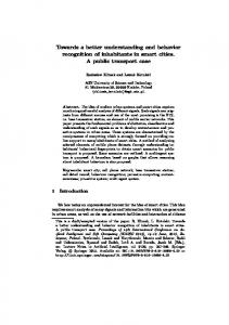
Figure 1. Idealised relationship between classification scale and homogeneity of soil map units (adapted by Pressey and Bedward (1991, p.8) from Beckett (1971)).

cation with the most distinct classes is the unworkable solution where every cell forms its own class. Secondly, the inherent continuous nature of environmental gradients and complexity of vegetation responses ensures that obvious breaks along environmental gradients at which boundaries can easily be drawn are rare. Thirdly, most traditional methods of unsupervised classification require users to artificially impose structure upon the data through the specification of the number of classes, the biophysical variables included and their weightings, and a dissimilarity measure or some other stopping criterion (Mackey and others 1988). Variation in these three elements can have a significant impact on the results of the classification process (Austin and Margules 1986; Belbin 1993). The best ELC of a landscape can be thought of as the classification with fewest classes that adequately captures environmental structure at the desired scale of analysis. The fewer classes there are, the less complex future planning and management will be. However, the fewer the classes, the more heterogeneous they are. It is important that classes do not become so broad that they group environments that are dissimilar enough to require different management treatments, or generalise special environments (e.g., rare and unusual environments). Within-class homogeneity has been found to increase sharply with increasing classification complexity at coarse scales of classification and tapers off at finer scales (Pressey and Bedward 1991; Bedward and others 1992; Figure 1). The homogeneity curve exhibits a spur at the medium/coarse classification scale, beyond which negligible increases in homogeneity are gained by increasing classification complexity. This suggests that this classification scale may be a fruitful place to search for the ecological land classification that optimally trades off classification complexity with class homogeneity. There are few tools available that are capable of automatically identifying the best ELC of a given landscape that are free from subjective decisions of the user. One of the few exam-

128

B. A. Bryan

Figure 2. Location map.

ples is by Burrough and others (2001) using fuzzy k-means techniques with partition coefficients and entropy statistics to select the best classification, although this is yet to be thoroughly tested in ELC. In this article, I assess the ability of a Bayesian classifier (AutoClass-C) to find the best classification of multivariate environmental data that automatically minimises classification complexity without unduly compromising class homogeneity. This is then compared with two synergistic techniques that facilitate multivariate data visualization (Self-Organising Map) and classification (kmeans classifier with homogeneity analysis). Unlike traditional methods (Belbin and MacDonald 1993), these techniques make no assumptions about the structure of data in terms of the number of classes or the degree of dissimilarity. The techniques are then integrated to test for synergistic benefits in finding the best ecological land classification of the Mt. Lofty Ranges.

Methods The Study Area and Environmental Data The Mt. Lofty Ranges study area (Figure 2) covers approximately 550,000 ha. The topography of the Ranges varies from gently undulating plains to intricately dissected ridges (Laut and others 1977). The climate is temperate, characterized by cool, wet winters and warm, dry summers with mean annual rainfall ranging from 400 to 1100 mm/yr (Laut and others 1977). The region forms the hinterland of the city of Adelaide that has a population of just over 1 million people and is subject to intense land use pressure from grazing, agriculture, horticulture, viticulture, water catchment, forestry, conservation, human settlement, and urban development. Land clearance has reduced the proportion of remnant native vegetation to less than 10%.

Synergistic Techniques for Ecological Land Classification

129

Figure 3. Maps of the five principal component data layers used in the ecological land classifications in this study.

The environmental data used for ELC in this study consists of the five GIS-based principal component (PC) data layers (Figure 3). The principal components were derived from a raster spatial database of 21 climatic (temperature and rainfall), topographic, solar radiation soil and solar radiation data layers created using a variety of spatial process models and data (Bryan 2000). The raster data layers consist of 2,060,290 grid cells of a resolution of 50 m. Assessment of the eigenvalues and eigenvectors of the principal components revealed that the first three principal components capture 88.7% of the variation in the original data. The first principal component that encapsulates more than 40% of the variation in the database is positively correlated with several temperature variables and inversely correlated with several rainfall variables (Table 1). The second PC is positively correlated with diurnal and annual temperature range, and the maximum temperature of the warmest period, and negatively correlated with rainfall seasonality (Table 1). PC 3 is positively correlated with

soil rockiness and PC 4 is negatively correlated with soil fertility. PC 5 displays a moderately strong inverse correlation with soil salinity (Table 1). The values of the five principal component layers are scaled according to the amount of variance captured in the original data layers (Table 2). AutoClass Bayesian Classifier AutoClass (NASA) is an automatic classifier (Hanson and others 1991) that uses Bayesian inference to derive the set of classes and class descriptions most likely to explain a given data set (Hanson and others 1991; see Cheeseman and Stutz 1996 for a thorough description). AutoClass has been extensively tested (Kanefsky and others 1991; 1994; Stutz and Cheeseman 1994; Cheeseman and Stutz 1996) and has been found to discover new, independently verified phenomena (Hanson and others 1991). The search technique used by AutoClass requires the user to specify a variety of initial class numbers. The

130

B. A. Bryan

Table 1. Correlations between principal components and input data layers Category

Environmental data layer

PC 1

PC 2

PC 3

PC 4

Temperature

Mean annual temperature Maximum temperature of the warmest period Minimum temperature of the coldest period Mean temperature of the driest quarter Mean temperature of the wettest quarter Diurnal temperature range Annual temperature range Minimum topographic temperature Maximum topographic temperature

0.961 0.073 0.844 0.797 0.929 )0.519 )0.506 0.947 0.665

0.039 0.863 )0.484 0.448 )0.270 0.799 0.808 )0.251 )0.180

)0.028 )0.271 0.143 )0.161 0.099 )0.252 )0.248 0.060 )0.042

)0.031 0.019 )0.033 )0.011 0.003 0.007 0.032 )0.061 )0.021

0.177 0.293 0.077 0.241 0.091 0.109 0.118 0.091 0.194

Rainfall

Mean annual rainfall Rainfall in driest period Rainfall in wettest period Rainfall Seasonality Annual Moisture Index

)0.803 )0.833 )0.735 )0.486 )0.885

)0.474 )0.326 )0.593 )0.713 )0.353

0.074 0.070 0.116 0.111 0.039

0.193 0.146 0.178 0.136 0.121

0.132 0.140 0.093 )0.045 0.020

Topographic

Soil Moisture Index

0.152

)0.010

)0.296

0.015

)0.183

Solar radiation

Relative short-wave radiation intensity

)0.003

0.018

)0.177

0.027

0.147

Soil

Soil Soil Soil Soil Soil

)0.147 0.578 0.044 )0.223 )0.058

)0.007 0.351 0.121 0.357 )0.382

0.104 0.225 )0.528 0.864 )0.687

)0.874 0.507 )0.013 )0.089 )0.062

)0.231 )0.375 )0.663 )0.094 )0.357

fertility pH salinity rockiness drainage

PC 5

Pearson correlation coefficients between principal components and input variables. Correlations greater than ±0.7 are displayed in bold.

Table 2. Descriptive statistics of the principal component data layers PC no. 1 2 3 4 5

Mean value

SD

Minimum

1457.6 936.2 754.8 757.9 1425.8

519.4 371.0 288.1 212.6 175.3

0 0 0 0 0

Maximum 2806.4 2034.4 1743.0 1336.2 1928.1

Descriptive statistics of the principal component data layers used as input into the ecological land classification techniques in this study.

program fits data iteratively to the stated number of classes and tests the posterior probability of the classification. AutoClass then uses a random log-normal function to select the number of classes for the next search trial according to the number of classes in the ‘‘best’’ classification so far—that which has the maximum posterior probability (Cheeseman and Stutz 1996). AutoClass converges data to the new number of classes and tests for probability in an iterative fashion. Hence, rather than just partitioning the desired number of classes within the database, the AutoClass Bayesian approach searches iteratively for the ‘‘best’’ classification and class descriptions based upon a specified error level. ‘‘A best classification optimally trades off predictive accuracy against the complexity of the classes, and so does not ÔoverfitÕ the data’’ (Hanson and others 1991; p. 1). Many searches of multivariate environmental data space were conducted with AutoClass to find the best

AutoClass ELC of the study area. AutoClass allows the user to specify relative error values for each attribute, which is a measure of the estimated error of measurement of each data attribute expressed as a percentage. The sensitivity of AutoClass to variation in relative error was systematically tested by using the converge search technique with input relative error values of 0.01%, 0.1%, 1%, 2%, 3%, 4%, 5%, 7%, and 9%, using initial class numbers of 10, 20, 40, 60, 80, and 100. Each AutoClass search was considered to have settled if the number of classes in the best classification was neither the highest nor lowest of the best 10 classifications found during the search. Kohonen Self-Organising Map The Self-Organising Map (SOM) is a special type of neural network developed for nonlinear mapping by (Kohonen 1995) and has been applied in a variety of fields (Bennani and others 1990; Dhawan and Arata

Synergistic Techniques for Ecological Land Classification

1993; Dolnicar 1997; Balastegui and others 2001). More recently, their use in ELC has been proven an effective method of classifying environments based on similar areas (Walley and OÕConnor 2001). The value of SOMs lies in their ability to uncover hidden structure in multidimensional data and enable its visualization in two dimensions by organising it into like regions in a two-dimensional map. SOMs are used in this study to visualise the inherent data structure in environmental data space so that an estimate of the number of classes can be made. This information is then used in conjunction with the k-means and homogeneity analysis techniques to select the best ELC of the study area. The SOM is based on a learning vector quantization algorithm. The SOM itself is usually a two-dimensional map or array of neurons and each neuron is a vector with n weights corresponding to the number of input variables. The SOM takes an input table of x rows (cases or grid cells) of n-dimensional multivariate data. Neurons in the SOM are trained over much iteration. During each training iteration, each case is presented to the SOM and the neuron closest to the input data case in multivariate data space is selected as the winner. Weight values of the winner neuron and those in a specified neighborhood around it are updated to be more like the input data case. Over time, both the neighborhood size and the learning rate decrease and the SOM stabilize. The outcome of this process is a two-dimensional SOM where nearby regions in the SOM occupy similar regions multivariate space. Kohonen (1995) should be consulted for the mathematics behind the SOM. Extensive testing of parameters required by the SOM including map dimensions, learning rates, training length, neighborhood size, and neighborhood topology was necessary before meaningful results could be obtained. The SOM_PAK (Kohonen and others 1996) software was used to initialize, train, test, and visualize SOMs in this study. Ultsch matrices (Ultsch 1993) are used to represent the topology of the SOM where neurons whose vectors are very different from their neighbors appear darker and neurons with similar neighbors are lighter colored. Thus, the number of distinct white regions in the SOM separated by dark boundaries gives an indication of the number of clusters/classes in the multidimensional environmental data. SOMs of dimension 100 · 50 neurons were considered appropriate for ELC in this study because they displayed an appropriate level of detail for the data and learning tended to settle more efficiently. Ten thousand training iterations were used in the organization phase and 1 million iterations for the training phase.

131

Learning rates used were reasonably high in the organization phase (0.5) and lower in the training phase (0.05–0.03) and better results were produced with a linear learning rate decrease function during the training phase. Neighborhoods of 70 neurons for the organization phase and 5 neurons for the training phase were used with a bubble neighborhood and rectangular topology. k-means with Homogeneity Analysis The k-means or ISOcluster unsupervised classification technique is one of the most common methods of unsupervised classification and is able to identify naturally occurring clusters of cells in the data space given a specified number of classes (Ball and Hall 1965; MacQueen 1967; Richards 1986). The ISO prefix reflects the Iterative Self Organising clustering method used, which calculates distances from all points to their nearest cluster centroid and iteratively updates the position of cluster centroids until this distance becomes minimal. A total of 24 ISOcluster classifications were created with the following class numbers: 1, 2, 3, 5, 7, 10, 12, 15, 20, 25, 30, 35, 39, 45, 50, 55, 60, 65, 70, 80, 90, 100, 120, and 150, using a sampling rate of 1 in every 25 cells. A maximum likelihood function was used to classify all cells in the study area according to their most likely class at all classification scales. Bedward and others (1992) propose a useful concept of homogeneity of ecological land classifications as the ratio of between-class variance to total variance. Bedward and others (1992) calculate homogeneity as a function of the pairwise association measures used in agglomerative classification. A major problem with pairwise strategies is that they are only suitable for a small number of cases because the pairwise association matrix quickly becomes extremely large. To avoid this problem, I assess homogeneity using the eta-squared statistic in a multivariate analysis of variance of ecological land classes. Eta-squared statistics are a measure of the ratio of within-group variance as a proportion of the total variance in the data. Eta-squared statistics are calculated for each of the classifications using PillaiÕs Trace, WilkÕs Lambda, HotellingÕs Trace, and RoyÕs Largest Root in the multivariate analysis of variance procedure in SPSS. The relationship between class homogeneity and classification complexity was used to select the best ecological land classification of the study area that has the smallest number of classes without compromising class homogeneity. Integration of Techniques The SOM, especially as represented by the Ultsch matrix, allows the visualization of the inherent com-

132

B. A. Bryan

Figure 4. Graphical representation of the relationship between relative error of input data and the number of classes in the best classification and the range of class numbers in the 10 best classifications found by AutoClass.

plexity of the multidimensional physical environmental data in two dimensions. The SOM also enables the integration of different classification techniques. ISOcluster classifications are mapped to the SOM by labeling each SOM neuron with the class number of the winning grid cell (the grid cell that is closest to the neuron in multidimensional principal component data space) as classified by the ISOcluster technique. In this way, we can visualize and assess the complexity of each classification against the backdrop of the SOM representation of the data structure. All of the ISOcluster classifications were mapped to the SOM to assist in interpreting the adequacy of classification with respect to the complexity of the underlying data.

Results Classification with AutoClass The number of classes in the single best classification and the range of class numbers of the 10 best classifications found by AutoClass under nine different relative error levels are presented in Figure 4. The two classifications with smallest error (relative error = 0.01% and 0.1%) had not reached local optima despite more than 1 week of processing time for each. Thus, classifications at 0.01% and 0.1% relative error were not considered for further analysis. At increased error levels however, the best classification tended to have class numbers in the middle of the range of the 10 best classifications found, suggesting that local optima had been reached. AutoClass classifications with relative error values of 3% and above also had problems in the form of unpopu-

lated classes. Thus, the validity of the process again broke down under moderate to high error levels, leaving only two valid AutoClass classifications at the 1% and 2% error levels (Figure 4). The 2% relative error classification (122 classes) was selected as the best AutoClass classification because of the lower number of classes. Analyses of these results revealed that the ability of AutoClass to find the best ELC of the study area was disappointing. Assessment of the 122-class AutoClass classification using dendrograms, bivariate plots, and analysis of entropy statistics suggests that there is significant overlap between classes. In addition, the variable most influential on the classification was PC 5, whereas the least influential was PC 1. This is undesirable because, as is commonly the case in PCA, PC1 contains many times more information than PC5, and hence should have the strongest influence on the classification. Visualizing Environmental Data Structure with the SOM The trained SOM (Figure 5) reveals the complex macro- and microstructure of the environmental data. To guide the reader, the Ultsch matrix represents neurons as black dots and the grey scale pixels represent the distance in environmental data space between adjacent neurons. Where the pixels are white, neighboring neurons represent similar physical environments. Conversely, where the pixels are darker, the environmental gradient between neurons is steeper. Thus, the white patches in the Ultsch matrix represent clusters of neurons with similar environments, and the

Synergistic Techniques for Ecological Land Classification

133

Figure 5. Ultsch matrix of the 100 · 50 neuron Kohonen self-organizing map of the environmental principal component data of the study area. Small black dots mark the position of each neuron, darker shades indicate greater differences between adjacent neurons, and lighter regions represent homogeneous data clusters.

darker veins running through the matrix can be used to distinguish between classes. Interpretation of distinct clusters in the SOM is a subjective process. The structure of the SOM as presented in the Ultsch matrix is complex, and there is no clear and obvious structure at any scale of assessment. There appears to be several large clusters (white areas) in the database that the Ultsch matrix represents as homogeneous light-colored regions defined by dark boundaries (Figure 5). Also present are many smaller, less well-defined clusters. Depending on the tendency and preference of the analyst either to detect broad patterns or fine scale detail, one could identify between 30 and 40 classes at the broad scale grading through to perhaps up to 100 classes at the fine scale (Figure 5). The complexity of the SOM reflects the complexity and continuous nature of the environmental data. The SOM has not clearly identified natural regions manifest as distinct clusters in the data. Classification with ISOcluster and Homogeneity Analysis A total of 24 different classifications of the study area were produced using ISOcluster with class numbers ranging from 2 to 150. Homogeneity analysis provided a means of understanding how each classification captures structure in environmental data. Homogeneity was found to vary with classification complexity in the same way that Bedward and others (1992) predict (Figure 6). The relationship between the four measures of homogeneity and class complexity does not provide unequivocal support for selecting a single best classification. However, it does enable the

visualization and understanding of the ability of each classification to capture the environmental complexity. Integrating Results The k-means with homogeneity analysis technique provides the most information about the structure of the data in multidimensional environmental space. Integration of the ISOcluster classifications with the SOM reveals a good level of agreement between the different techniques. Homogeneous zones in the SOM tended to be labeled with the same class number, and neurons separated by darker pixels in the Ultsch matrix tend to have different class labels. However, there is some disagreement between the techniques that reflect a higher level of data structure captured by the SOM relative to that captured by the ISOcluster classifications. The evidence for this was twofold. Firstly, some Autoclass and ISOcluster classes appear in two different regions of the SOM. Secondly, in some cases the same class labels spanned the darker region boundaries of the SOM. An example is provided of the integration of the 50-class ISOcluster classification within the SOM (Figure 7). Selecting an Ecological Land Classification Using the information provided by the homogeneity analysis and the SOM to select a final classification is a subjective process. The selection of a single optimal classification that trades off class homogeneity and classification complexity requires the development of functions that quantify the benefit of homogeneity and the costs of classification complexity in dollar terms or some other comparable unit. Development of robust

134

B. A. Bryan

Figure 6. Graphical representation of the relationship between class homogeneity as calculated using the eta-squared statistic, and class complexity as defined by the number of classes derived by the ISOcluster process.

functions for these parameters is very difficult and may be a fruitful avenue for future research. Without these functions, there is no clear and obvious way to help guide the selection of a single classification. Pragmatically, it may be useful to adopt a decision theory approach to the problem of selecting a single classification for use in environmental management. The classification selection decision depends on the desired scale of future analyses and management treatments, and the level of complexity and generalization of detail acceptable to the manager. Also, the decision of level of classification complexity depends on the marginal benefits of increasing class homogeneity relative to the marginal costs of increasing classification complexity. The decision processes of the environmental manager in selecting a particular classification can be bound by two extremes:

1.

2.

Coarse Scale Classification—where the marginal costs of increasing class complexity outweigh the marginal benefits of increasing class homogeneity. Hence, a low classification complexity is more important than high class homogeneity. Fine Scale Classification—where the marginal benefits of increasing class homogeneity outweigh the marginal costs of increasing class complexity. Hence, high class homogeneity is more important than low classification complexity.

In the Coarse Scale case above, the environmental manager wishes to select the classification with the fewest classes that has the minimum acceptable level of class homogeneity. Pragmatically, this could be done by following the homogeneity curve from left to right (in order of increasing classification complexity) and

selecting the classification after which the marginal improvements in homogeneity begin to decrease (i.e., maybe around the 15–20 class level). This kind of classification may be required where there is a high marginal cost of increasing classification complexity relative to the benefits in increased class homogeneity such as in defining broad natural resource management administrative regions. In this example, each extra region defined requires significant expenditure in terms of office space, administrative personnel, and office equipment, and so on. In the Fine Scale case above, the environmental manager wishes to select the classification at the maximum level of class homogeneity beyond which the level of classification complexity outweighs the very small marginal gains in homogeneity. Again, pragmatically, this could be done by following the homogeneity curve from left to right (in order of increasing classification complexity) and selecting the classification after which the marginal improvements in homogeneity become negligible (i.e., perhaps around the 50– 70 class level (Figure 6). This kind of classification may be required in cases where the marginal cost of increasing classification complexity is low relative to the benefits such as in the analysis of biodiversity. In this example, it may be important to have a fine scale classification that captures most of the physical environmental variation. The cost of high classification complexity is low because it simply means a few more rows in the analysis for the research scientist. The environmental manager could reasonably justify selection of either of these two extreme classification scales. They could just as easily justify any scale of classification in between these extremes, depending on the ratio of marginal benefit of increasing class

Synergistic Techniques for Ecological Land Classification

homogeneity to the marginal cost of increasing classification complexity. Despite all of the above analysis, the selection of a single classification remains a subjective exercise. However, information gained from the classification techniques and the integration of different techniques presented in this study can inform the selection of a good classification suitable for use in environmental research and management. As the purpose of the classification of the environments of the Mt. Lofty Ranges is intended for use primarily in ecological assessment and revegetation planning, the marginal benefits of increasing class homogeneity outweigh the marginal costs of increasing classification complexity somewhat. Hence, the 50-class ISOcluster classification is a reasonable choice because there seems to be negligible marginal improvements to be made in class homogeneity beyond this level, especially considering the RoyÕs Largest Root measure or homogeneity. Integration and assessment of the Autoclass and ISOcluster classifications with the SOM revealed that the 50-class classification captured the broad and medium scale structural detail evident in the SOM. Hence, the 50-class scale of classification is selected for use in future applied ecological research in the Mt. Lofty Ranges. Mapping and analysis of the spatial structure of ecological land classes reveals that cells of the same class tend to be clumped together in the landscape, resulting in a good level of class cohesiveness in geographic space (Figure 8). This is expected because of the high level of spatial autocorrelation common in spatial data. Many ecological land classes occur as spatially contiguous regions, and several also have more than one distinct patch distributed in different parts of the landscape. This high level of cohesive geographic regionalization makes future research and management based on the ecological land classifications much simpler than dealing with highly disaggregated spatial units.

Discussion The results of multivariate analyses are notoriously opaque because of the high dimensionality of the data and the difficulty of visualization. Often, there is very little comparison between methods, and checks of classification validity are rare (Thompson and others 2004). This study compares the processes of finding the best ELC of the study area using three independent, quantitative techniques. The results of this study do not disagree with the ability of the AutoClass Bayesian classification technique to automatically find the classification that

135

optimally trades off classification complexity with class homogeneity. AutoClass may perform much better on data with much more distinct class breaks rather than the complex and continuous nature of the environmental data in this study. In practice, AutoClass was found not to be robust to changes in relative error of input data. With some testing, it was possible to identify the relative error limits within which sensible classifications could be obtained. Selection of different relative error levels within these limits however, resulted in different levels of classification complexity being assessed as the best classification. Hence, subjective choices can still affect the resulting classification even when purpose-built optimal classification techniques such as AutoClass are employed. This leads to the seemingly unavoidable situation where some subjectivity is always required in classifying elements lying along continuous gradients into rigid classes. If indeed this is the case, it follows that this subjectivity should be explicit and guided by the best possible information about the multidimensional structure of the data rather than relying on adjusting some arbitrary measure of relative error or other measure of fuzziness or stopping criterion. The SOM provides a two-dimensional visualization of the multidimensional structure of the data that can then assist the subjective decision-making that surrounds the classification complexity/class homogeneity tradeoff. The SOM stops short of actually assigning input data vectors to classes, and thus avoids difficulties associated with optimal classification. Rather, the SOM is much more profitably used as a tool for suggesting appropriate levels of classification complexity. Substantial user subjectivity is required to assess appropriate levels of classification complexity for the data. The classical k-means or ISOcluster technique is an established and accepted method for finding the optimal clustering of data points at a given scale of classification. The creation of k-means classifications at a variety of scales and analysis of the homogeneity of classes proved to be a simple, transparent, and elegant means of investigating the multidimensional structure of the data. Unlike the fuzzy-based measures of Burrough and others (2001), homogeneity analysis is not able to select the best ELC. Like the SOM, it is best used to guide the subjective choices of the user. The 50-group optimal ISOcluster classification was considered the classification with fewest classes that did not sacrifice the homogeneity of environment types and hence was selected for use in further ecological research in the Mt. Lofty Ranges study area. The 50-class classification captured most of the structural detail evident in the SOM. Hence, it is considered the most appropriate

136

B. A. Bryan

Figure 7. Integration of the selforganizing map (represented by the grey scale image of the Ultsch matrix) with the 50 environment types identified by the 50-class ISOcluster classification (superimposed class numbers).

Synergistic Techniques for Ecological Land Classification

137

Figure 8. Example of the spatial distribution of ecological land classes of the 50-class ISOcluster classification. Land classes are shaded in different shades of gray and underlain by landscape topography.

classification on which to base further environmental research, management, and decision-making. The results of this study support the assertion of Austin and Smith (1989) and Belbin (1993) that if continuum theory is correct, then any attempt at determining the optimal number of classes in land classification may be defeated. Physical environmental parameters occur more or less as continua in the landscape. Despite the ease at which natural regions can be seen in the landscape, the data may not capture the homogeneity and heterogeneity so freely observed. The technical endeavor of finding the classification of multivariate data that optimally trades off classification complexity and class homogeneity is difficult and plagued by assumptions. The general paucity of tools available for optimal classification is a manifestation of these difficulties. The results from AutoClass suggest that there may be little alternative to the user selecting a desired scale

of classification. There may not be natural regions in multivariate physical environmental data. It follows then that the goals of ELC—to find the assumptionfree classification that optimally trades off classification complexity with class homogeneity—may be unachievable. It may be more useful to accept that there is no single optimal classification, but many good classifications at a variety of scales. Furthermore, there appears to be a scale of classification beyond which the marginal benefits of increasing the classification complexity are not worth the marginal gains in class homogeneity, but defining precisely where the cut-off point would be a subjective decision. The SOM and kmeans with homogeneity analysis techniques accept this reality of classification and help inform this decision process with information about the data structure. The automation of these techniques in an ELC package can comprise a transparent and explicit means of creating ELCs (Hargrove and Hoffman 2004). The

138

B. A. Bryan

further testing of other optimal classification techniques such as fuzzy k-means (Burrough and others 2001) and the use of information theory (Kraft and others 2004) is another potentially fruitful area of further research and development in ELC.

Conclusion

mary Industries and Resources and PlanningSA. I am grateful to Professor Hugh Possingham for reading an early version of this work and to Neville Crossman and Dave Gerner for comments on the final draft. Infrastructure and support from GISCA, the National Centre for Social Applications of GIS, University of Adelaide is gratefully acknowledged. This research was supported by an Australian Postgraduate Research Award scholarship and an Australian Research Council Discovery Project grant DP0343036. CSIRO Land and Water also contributed to the final revision of this article.

This application of the AutoClass Bayesian classifier is the first application of this new technique to ELC. However, the technique is not free from assumptions that significantly affect the best classification found by AutoClass. AutoClass has had success in finding natural classifications in other application areas. The inability of this technique to find the best ELC of the study area is not a slight on the technique but rather confirmation that the natural regions we see in the landscape are difficult to capture using landscape scale multivariate physical environmental data. Furthermore, the continuous nature of these data gradients mean that it is impossible to find the best ELC without some level of subjectivity affecting the scale and complexity of classification. Hence, the predilection of environmental managers for discrete planning units in the form of an ELC is at odds with the inherently continuous nature of environmental gradients, and better techniques are required to create ELCs at scales that best trade off classification complexity with class homogeneity. A fruitful avenue of research is in the quantification and comparison of the marginal benefits of increasing class homogeneity and the marginal costs of increasing classification complexity and its use in selecting optimal classifications. The SOM has the ability to abstract and visualize multidimensional data in a two-dimensional array and thereby provide the user with a visual indication of the data structure. Integration of the SOM with ecological land classifications created by ISOcluster provided synergistic benefits in allowing the visualization of the classification against the structure of the data as represented in the SOM. Homogeneity analysis and its application to ISOcluster classifications at a variety of scales also provide an elegant and transparent means of selecting the best ELC of the study area. Automating this technique would provide environmental managers with a simple and robust way to create environmental classifications that trade off classification complexity for class homogeneity.

Bennani, Y., F. Fogelman-Soulie´ , and P. Gallinari. 1990. Textdependent speaker identification using learning vector quantization. Pages 1087–1090 in Proceedings of INNCÕ90, International Neural Network Conference II, Kluwer Academic Press.

Acknowledgments

Brandt, J., E. Holmes, and D. Larsen. 1994. Monitoring ÔSmall BiotopesÕ. Pages 251–274 in F. Klijn (ed.), Ecosystem classification for environmental management. Kluwer Academic Press, Dordrecht.

The author gratefully acknowledges the use of data supplied by the South Australian Department of Pri-

Bryan, B. A. 2000. Strategic revegetation planning in an agricultural landscape: a spatial information technology

Literature Cited Abella, S. R., V. B. Shelburne, and N. W. Macdonald. 2003. Multifactor classification of forest landscape ecosystems of Jocassee Gorges, Southern Appalachian Mountains, South Carolina. Canadian Journal of Forest Research-Revue Canadienne De Recherche Forestiere 33:1933–1946. Austin, M. P., and C. R. Margules. 1986. Assessing representativeness. Pages 45–67 in M. B. Usher (ed), Wildlife conservation evaluation. Chapman and Hall, London. Austin, M. P., and T. M. Smith. 1989. A new model for the continuum concept. Vegetatio 83:35–47. Bailey, R. G. 1996. Ecosystem geography. Springer-Verlag, New York. Bailey, R. G. 2004. Identifying ecoregion boundaries. Environmental Management 34(Suppl 1):S14–S26. Balastegui, A., P. Ruiz-Lapuente, and R. Canal. 2001. Reclassification of gamma-ray bursts. Monthly Notices of the Royal Astronomical Society 328:283–290. Ball, G. H., and D. J. Hall. 1965. A novel method of data analysis and pattern classification. Stanford Research Institute, Menlo Park, California. Bedward, M., D. A. Keith, and R. L. Pressey. 1992. Homogeneity analysis: assessing the utility of classifications and maps of natural resources. Australian Journal of Ecology 17:133–139. Belbin, L. 1993. Environmental representativeness: regional partitioning and reserve selection. Biological Conservation 66:223–230. Belbin, L., and C. McDonald. 1993. Comparing three classification strategies for use in ecology. Journal of Vegetation Science 4:341–349.

Synergistic Techniques for Ecological Land Classification

approach. PhD dissertation, University of Adelaide, South Australia. Bunce, R. G. H., C. J. Barr, R. T. Clarke, D. C. Howard, and A. M. J. Lane. 1996. Land classification for strategic ecological survey. Journal of Environmental Management 47:37–60. Bunce, R. G. H., P. D. Carey, R. Elena-Rossello, J. Orr, J. Watkins, and R. Fuller. 2002. A comparison of different biogeographical classifications of Europe, Great Britain and Spain. Journal of Environmental Management 65:121–134. Burrough, P. A., P. F. M. van Gaans, and R. A. MacMillan. 2000. High-resolution landform classification using fuzzy kmeans. Fuzzy Sets and Systems 113:37–52. Burrough, P. A., J. P. Wilson, P. F. M. van Gaans, and A. J. Hansen. 2001. Fuzzy k-means classification of topo-climatic data as an aid to forest mapping the Greater Yellowstone Area, USA. Landscape Ecology 16:523–546. Carmean, W. H. 1996. Forest site-quality estimation using forest ecosystem classification in Northwestern Ontario. Environmental Monitoring and Assessment 39:493–508. Carter, R. E., M. D. MacKenzie, and D. H. Gjerstad. 1999. Ecological land classification the Southern Loam Hills of South Alabama. Forest Ecology and Management 114:395–404. Cheeseman, P., and J. Stutz. 1996. Bayesian classification (AutoClass): theory and results. Pages 153–180 in U. M. Fayyad, G. Piatetsky-Shapiro, P. Smyth, and R. Uthurusamy (eds.), Advances knowledge discovery and data mining. AAAI Press/MIT Press. Chon, T., Y. Park, and J. H. Park. 2000. Determining temporal pattern of community dynamics by using supervised learning algorithms. Ecological Modelling 132:151–166. Christian, C. S., and G. A. Stewart. 1968. Methodology of integrated surveys. UNESCO, Paris. Claessen, F. A. M., F. Klijn, J. Flip, P. M. Witte, and J. G. Nienhaus. 1994. Ecosystem classification and hydro-ecological modelling for national water management. Pages 199–222 in F. Klijn (eds.), Ecosystem classification and environmental management. Kluwer Academic Press, Dordrecht. Dhawan, A. P., and L. Arata. 1993. Segmentation of medical images through competitive learning. Pages 1277–1282 in Proceedings of ICNNÕ93, International Conference on Neural Networks III, IEEE Service Center. Dolnicar, S. 1997. The use of neural networks marketing: market segmentation with self organising feature maps. Pages 38–43 in Proceedings of WSOMÕ97, Workshop on Self-Organizing Maps, Helsinki University of Technology, Neural Networks Research Centre, June 4–6, 1997, Espoo, Finland.

139

Hargrove, W., and F. M. Hoffman. 2004. Potential of multivariate quantitative methods for delineation and visualization of ecoregions. Environmental Management 34(Suppl 1):S39–S60. Hill, M. O. 1979. TWINSPAN: a FORTRAN program for arranging multivariate data in an ordered two-way table by classification of the individual and attributes. Cornell University Press, Ithaca, New York. Hirvonen, H. 2001. CanadaÕs national ecological framework: an asset to reporting on the health of Canadian forests. Forestry Chronicle 77:111–115. Host, G. E., P. L. Polzer, D. J. Mladenoff, M. A. White, and T. R. Crow. 1996. A quantitative approach to developing regional ecosystem classifications. Ecological Applications 6:608–618. Hutto, C. J., V. B. Shelburne, and S. M. Jones. 1999. Preliminary ecological land classification of the Chauga Ridges region of South Carolina. Forest Ecology and Management 114:385–393. Kanefsky, B., J. Stutz, and P. Cheeseman. 1991. An automatic classification of a Landsat/TM image from Kansas (FIFE). Technical report FIA-91-26, NASA Ames Research Center, Artificial Intelligence Branch. Kanefsky, B., J. Stutz, P. Cheeseman, and W. Taylor. 1994. An improved automatic classification of a Landsat/TM image from Kansas (FIFE). Technical report FIA-94-01, NASA Ames Research Center, Artificial Intelligence Branch. Kirkpatrick, J. B., and M. J. Brown. 1994. A comparison of direct and environmental domain approaches to planning reservation of forest higher plant communities and species Tasmania. Conservation Biology 8:217–224. Kohonen, T. 1995. Self-organizing maps. Springer Series Information Science 30. Kohonen, T., J. Hynninen, J. Kangas, and J. Laaksonen. 1996. SOM_PAK: the self-organizing map program package. Report A31. Helsinki University of Technology, Laboratory of Computer and Information Science, Espoo, Finland. Kraft, J., J. W. Einax, and C. Kowalik. 2004. Information theory for evaluating environmental classification systems. Analytical and Bioanalytical Chemistry 380:475–483. Kupfer, J. A., and S. B. Franklin. 2000. Evaluation of an ecological land type classification system, Natchez Trace State Forest, Western Tennessee, USA. Landscape and Urban Planning 49:179–190. Lathrop, R. G., and J. A. Bognar. 1998. Applying GIS and landscape ecological principles to evaluate land conservation alternatives. Landscape and Urban Planning 41:27–41.

Franklin, J. 2003. Clustering versus regression trees for determining ecological land units in the Southern California Mountains and Foothills. Forest Science 49:354–368.

Laut, P., P. C. Heyligers, G. Keig, E. Loffler, C. Margules, R. M. Scott, and M. E. Sullivan. 1977. Environments of South Australia, Province 3 Mt. Lofty Block. CSIRO Division of Land Use Research, Canberra.

Gallant, A. L., T. R. Loveland, T. L. Sohl, and D. E. Napton. 2004. Using an ecoregion framework to analyze land-cover and land-use dynamics. Environmental Management 34(Suppl 1):S89–S110.

Leathwick, J. R., J. M. Overton, and M. Mcleod. 2003. An environmental domain classification of New Zealand and its use as a tool for biodiversity management. Conservation Biology 17:1612–1623.

Hanson, R., J. Stutz, and P. Cheeseman. 1991. Bayesian classification theory. Technical report FIA-90-12-7-01, NASA Ames Research Center, Artificial Intelligence Branch.

Legendre, P., and A. Vaudor. 1991. Le progiciel R. analyse multidimensionnelle, analyse spatiale. UserÕs guide. Universite´ de Montre´ al, Montre´ al.

140

B. A. Bryan

Lek, S., and J. F. Gue´ gan. 1999. Artificial neural networks as a tool in ecological modelling: an introduction. Ecological Modelling 120:65–73.

Omernik, J. M. 2004. Perspectives on the nature and definition of ecological regions. Environmental Management 34(Suppl 1):S27–S38.

Lindenmayer, D. B., and R. B. Cunningham. 1996. A habitatbased microscale forest classification system for zoning wood production areas to conserve a rare species threatened by logging operations south-eastern Australia. Environmental Monitoring and Assessment 39:543–557.

Park, Y., R. Ce´ re´ ghino, A. Compin, and S. Lek. 2003. Applications of artificial neural networks for patterning and predicting aquatic insect richness running waters. Ecological Modelling 160:265–280.

Lioubimtseva, E., and P. Defourny. 1999. GIS-based landscape classification and mapping of European Russia. Landscape and Urban Planning 44:63–75. Loveland, T. R., and J. M. Merchant. 2004. Ecoregions and ecoregionalization: geographical and ecological perspectives. Environmental Management 34(Suppl 1):S1–S13. Mabbutt, J. A. 1968. Aeolian landforms in Central Australia. Australian Geographical Studies 6:139–150. Mackey, B. G. 1993. A spatial analysis of the environmental relations of rainforest structural types. Journal of Biogeography 20:303–336. Mackey, B. G., H. A. Nix, M. F. Hutchinson, J. P. MacMahon, and P. M. Fleming. 1988. Assessing representativeness of places for conservation reservation and heritage listing. Environmental Management 12:501–514. Mackey, B. G., H. A. Nix, J. A. Stein, S. E. Cork, and F. T. Bullen. 1989. Assessing the representativeness of the wet tropics of Queenslands World Heritage property. Biological Conservation 50:279–303. MacMillan, R. A., W. W. Pettapiece, S. C. Nolan, and T. W. Goddard. 2000. A generic procedure for automatically segmenting landforms into landform elements using DEMs, heuristic rules and fuzzy logic. Fuzzy Sets and Systems 113:81–109. MacQueen, J. B. 1967. Some methods for the classification and analysis of multivariate observations. Pages 281–297 in L. Le Cam and J. Neyman (eds.), Proceedings of the Fifth Berkeley Symposium on Mathematical Statistics and Probability 1. University of California Press, Berkeley, CA. McKenney, D. W., B. G. Mackey, and R. A. Sims. 1996. Primary databases for forest ecosystem management—examples from Ontario and possibilities for Canada: NatGRID. Environmental Monitoring and Assessment 39:399–416. Nadeau, L. B., C. Li, and H. Hans. 2004. Ecosystem mapping in the lower foothills subregion of Alberta: application of fuzzy logic. Forestry Chronicle 80:359–365. Neily, P. D., E. Quigley, L. Benjamin, B. Stewart, and T. Duke. 2003. Ecological land classification for Nova Scotia: volume 1—mapping Nova ScotiaÕs terrestrial ecosystems. Report DNR 2003-2, April 2003, Nova Scotia Department of Natural Resources, Renewable Resources Branch.

Pressey, R. L., and M. Bedward. 1991. Mapping the environment at different scales: benefits and costs for nature conservation. Pages 7–13 in C.R. Margules, M.P. Austin (eds.), Nature conservation: cost effective biological surveys and data analysis. CSIRO, Australia. Pressey, R. L., and V. S. Logan. 1994. Level of geographical subdivision and its effects on assessments of reserve coverage—a review of regional studies. Conservation Biology 8:1037–1046. Pressey, R. L., and V. S. Logan. 1995. Reserve coverage and requirements relation to partitioning and generalization of land classes—analyses for western New South Wales. Conservation Biology 9:1506–1517. Richards, J. A. 1986. Remote sensing digital image analysis: an introduction. Springer-Verlag, New York. Runhaar, H. J., and H. A. Udo de Haes. 1994. The use of site factors as classification characteristics for ecotopes. Pages 169– 172 in F. Klijn (eds.), Ecosystem classification for environmental management. Kluwer Academic Press, Dordrecht. Sims, R. A., I. G. W. Corns, and K. Klinka. 1996. Global to local: ecological land classification. Environmental Monitoring and Assessment 39:1–10. Stutz, J., and P. Cheeseman. 1994. AutoClass—a Bayesian approach to classification. In J. Skilling and S. Sibisi (eds.), Maximum entropy and Bayesian methods. Kluwer Academic Press, Dordrecht. Thompson, R. S., S. L. Shafer, K. H. Anderson, L. E. Strickland, R. T. Pelltier, P. J. Bartlein, and M. W. Kerwin. 2004. Topographic, bioclimatic, and vegetation characteristics of three ecoregion classification systems in North America: comparisons along continent-wide transects. Environmental Management 34(Suppl 1):S125–S148. Ultsch, A. 1993. Self organized feature maps for monitoring and knowledge acquisition of a chemical process. Pages 864–867 in S. Gielen, B. Kappen (eds.), Proceedings of the international conference on artificial neural networks (ICANN93). Springer-Verlag, London. Walley, W. J., and M. A. OÕConnor. 2001. Unsupervised pattern recognition for the interpretation of ecological data. Ecological Modelling 146:219–230. Watts, D. 1970. Principles of biogeography. McGraw-Hill, New York.

Nix, H. A. 1982. Environmental determinants of biogeography and evolution Terra Australis. pages: 47–66 In W. R. Barker and P. J. M. Greenslade (eds.), Evolution of the flora and fauna of arid Australia. Peacock Publications. .

Wolock, D. M., T. C. Winter, and G. McMahon. 2004. Delineation and evaluation of hydrologic-landscape regions in the United States using geographic information system tools and multivariate statistical analyses. Environmental Management 34(Suppl 1):S71–S88.

Nolet, P., G. Domon, and Y. Bergeron. 1995. Potentials and limitations of ecological classifications as a tool for forest management: a case study of disturbed deciduous forests, Que´ bec. Forest Ecology and Management 78:85–98.

Zonneveld, I. 1994. Basic principles of classification. Pages 23–48 in F. Klijn (ed), Ecosystem classification for environmental management. Kluwer Academic Press, Dordrecht.