Synthesis of Constrained nR Planar Robots to Reach Five Task Positions Gim Song Soh
J. Michael McCarthy
Robotics and Automation Laboratory University of California Irvine, California 92697-3975 Email:
[email protected]
Department of Mechanical and Aerospace Engineering University of California Irvine, California 92697-3975 Email:
[email protected]
Abstract— In this paper, we design planar nR serial chains that provide one degree-of-freedom movement for an end-effector through five arbitrarily specified task positions. These chains are useful for deployment linkages or the fingers of a mechanical hand. The trajectory of the end-effector pivot is controlled by n-1 sets of cables that are joined through a planetary gear system to two input variables. These two input variables are coupled by a four-bar linkage, and the movement of the end-effector around its end joint is driven by a second four-bar linkage. The result is one degree-of-freedom system. The design of the cabling system allows control of the shape of the chain as it moves through the task positions. This combines techniques of deployable linkage design with mechanism synthesis to obtain specialized movement with a minimum number of actuators. Two example designs for a 6R planar chain are presented, one with a square initial configuration and a second with a hexagonal initial configuration.
I. I NTRODUCTION In this paper, we present a methodology for the design of planar nR serial chains such that the end-effector reaches five arbitrary task positions with one degree-of-freedom. The method is general in that we may introduce mechanical constraints between m drive joints and n−m driven joints. For the purposes of this paper, we consider m = 1, and show how to use cables combined with planetary gear trains to constrain the end-effector movement to three degrees-of-freedom. Then, we design four-bar chains attached at the base and at the endeffector to obtain a one degree-of-freedom system. See Figure 1. As an example, we obtain a one degree-of-freedom 6R planar chain that reaches five specified task positions. This work can be used to control the shape of deployable chains, as well as for the design of mechanical fingers for specialized grasping. II. L ITERATURE R EVIEW Cable systems are employed to reduce the inertia of a manipulator system by permitting the actuators to be located remotely, thus a higher power-to-weight ratio over a direct drive system, see Lee (1991) [1]. Recent work on cabledriven robotic systems includes Arsenault and Gosselin (2006) [2], who introduce a 2-dof tensegrity mechanism to increase the reachable workspace and task flexibility of a serial chain robot. Also, Lelieveld and Maeno (2006) [3] present a 4 DOF
H Cn-2
G
Cn-2
Cn-1 C n
Cn-1
Cn
C3 C3 C2 C1
C2 C1 Base Pulleys
Planetary Gear Train
Fig. 1. The Design Problem. The figure on the left shows a schematic of planar nR serial robot, and the figure on the right shows a schematic of the constrained nR robot.
portable haptic device for the index finger driven by a cableactuated rolling-link-mechanism (RLM). Palli and Melchiorri (2006) [4] explore a variation on cables using a tendon sheath system to drive a robotic hand. Our work is inspired by Krovi et al. (2002) [5], who present a synthesis theory for nR planar serial chains driven by cable tendons. Their design methodology sizes the individual links and pulley ratios to obtain the desired end-effector movement used to obtain an innovative assistive device. Our approach borrows from deployable structures research Kwan and Pelligrino (1994) [6], and uses symmetry conditions to control the overall movement of the chain, while specialized RR cranks position the base and end-effector joints. For our serial chain the designer can choose the location of the base joint C1 , the attachment to the end-effector Cn , and the dimensions of the individual links which for convenience we assume are the same size. See Figure 1. Our goal is to design the mechanical constraints that ensures the end-effector reaches each of five task positions, in response to an input drive variable. This research extends the ideas presented in Leaver and McCarthy (1987) [7] and Leaver et al. (1988) [8] using the tendon routing analysis of Lee (1991) [1]. Also see Tsai (1999) [9]. While our proposed system appears complicated,
Writing (2) once for each of the tendon routing k, k = 1, . . . , n for an nR serial robot, yields the following linear transformation in matrix form:
it has only one actuator. III. T HE P LANAR N R S ERIAL C HAIN ROBOT Let the configuration of an nR serial chain be defined by the coordinates Ci = (xi , yi ), i = 1, . . . , n to be each of its revolute joints. See Figure 1. The distances ai,i+1 = |Ci+1 − Ci | defined the lengths of each link. Attach a frame Bi to each of these links so its origin is located at Ci and its x axis is directed toward Ci+1 . The joints C1 and Cn are the attachments to the base frame F = B1 and the moving frame M = Bn , respectively, and we assume they are the origins of these frames. The joint angles θi define the relative rotation about the joints Ci . Introduce a world frame G and task frame H so the kinematics equations of the nR chain are given by [D] = [G][Z(θ1 )][X(a12 )] . . . [X(an−1,n )[Z(θn )][H],
(1)
where [Z(θi )] and [X(ai,i+1 )] are the 3 × 3 homogeneous transforms that represent a rotation about the z-axis by θi , and a translation along the x-axis by ai,i+1 , repspectively. The transformation [G] defines the position of the base of the chain relative to the world frame, and [H] locates the task frame relative to the end-effector frame. The matrix [D] defines the coordinate transformation from the world frame G to the task frame H. IV. K INEMATICS OF T ENDON D RIVEN ROBOTS The relationship between the rotation of the base pulley and the joint angles in an open-loop chain with (k+1) links can be described by: θk∗ = θ1 ± (
rk,i rk,k rk,2 )θ2 ± . . . ( )θi ± . . . ( )θk , rk rk rk
(2)
where θk∗ denotes the base pulley angle of the k th tendon, θi denotes the joint angle of the ith joint, rk,i denotes the radius of the pulley of the ith joint of the k th tendon, and rk denotes the radius of the base pulley of the k th tendon. The r sign of each term, ( rk,i )θi , in (2) is to be determined by the k number of cross-type routing preceding the ith joint axis. If the number of cross-type routing is even, the sign is positive, else it is negative. See the connection between C1 and C2 of Tendon 3 in Figure 2 for an example of cross-type routing. For derivation of this equation, refer to Lee (1991) [1].
Tendon 1:
θ1*
θ2* Tendon 2: * Tendon 3: θ3
r1,1 1 r2,2
r2,1 1 r3,1 C1
1
2 r3,3
r3,2 2 C2
3
C3
Fig. 2. Planar schematic for a three-DOF planar robot with structure matrix (5).
Θ∗ = [B][R]Θ.
(3)
∗
= (θ1∗ , θ2∗ , . . . , θn∗ )T denotes (θ1 , θ2 , . . . , θn )T denotes the
where Θ the base pulley angles and Θ = joint angles. If we let rk,j = rk , k = 1, . . . , n such that all the pulleys have the same diameter, then [B][R] would be reduced to a lower triangular n × n matrix with entries +1 or −1, 1 0 0 ... 0 1 ±1 0 . . . 0 (4) [B][R] = [B] = . .. .. .. . .. . . ... . 1 ±1 ±1 . . .
±1
The matrix [B] is known as the structure matrix, Lee (1991) [1]. It describes how the tendons are routed. The matrix [R] is a diagonal scaling matrix with elements representing the ratio of the radii of the i-th joint pulley to the i-th base pulley. In this paper, we size the pulleys to be of equal lengths such that this matrix is the identity. We illustrate with an example on constructing the tendons of a 3R serial robot from the structure matrix. Suppose the structure matrix, [B] is defined to be 1 0 0 0 . (5) [B] = 1 1 1 −1 −1 Each columns of the matrix [B] corresponds to the routing prior to the joint pivots, and each row represent an independent tendon drive. The element in the first row is always +1 since we are driving the fixed pivot C1 directly with θ1∗ . For the second row, it represent a parallel-type routing between the moving pivot C2 and fix pivot C1 since the sign of the second element remains unchanged. For the last row, the second element changes sign, we get a cross-type between the moving pivot C2 and fix pivot C1 . Also, the sign remains unchanged after the second element, parallel-type follows between the moving pivot C3 and C2 . See Figure 2 for the planar schematic for the structure matrix (5). V. S CHEMATIC OF A CONSTRAIN N R P LANAR ROBOT The schematic of a constrain nR Planar Robot consists of a nR serial chain, N −1 tendons, a planetary gear train, and two RR chains. See Figure 3. Our goal is to use the N −1 tendons, a planetary gear train, and two RR chains to mechanically constrain a specified nR serial chain that reaches five task position to one degree-of-freedom. The N − 1 base pulleys were connected to the N − 1 tendons to group the actuation point to the base for easy attachment to a planetary gear train. The specified nR serial chain have n degrees of freedom. The attachment of the N − 1 tendons to the nR serial chain does not change the system degrees of freedom, but it allows the control of the first n − 1 joint angles from the base independently. If we add a planetary gear train to couple the various n − 1 base pulleys as shown in Figure 5, we are able
τ2
nR τ2
τ2
τ2
τ2
θn
[A] = [B]−1 [S][C].
(7)
[B] is a matrix that describes the relationship between the relative joint angles and the rotation of the base pulleys, see (3). [S] is a diagonal matrix that scales the sum of the row elements of matrix [C] to unity. This matrix was included to account for the effects of changing the size of the base pulleys and is the ratio of the ith base pulley to the ith joint pulley. [C] is a matrix that describes the relationship between the rotation of the base pulleys to the inputs of the transmission system.
τ2 τ1
Base Pulleys
so we obtain the desired coupling matrix [A] in the relation
∗
θi , i = 1, 2, ..., n-1
Planetary τ , τ Gear Train 1 2 Fig. 3. Schematic for a constrain nR Planar Robot driven by cables, mechanically constraint by planetary gear train and RR cranks.
to reduce the tendon driven robot to a three degree-of-freedom system. Two RR constraints were then added to obtain a one degree-of-freedom system. The first RR chain serves to couple the planetary gear train inputs τ1 and τ2 together, and the purpose of the second RR chain is to couple the nth joint, θn , to τ2 and hence τ1 . As shown in Figure 3, if we denote τ1 as the input that drive the first joint angle, we can see that τ2 is related to the input τ1 through the four bar linkage formed from the attachment of an RR constraint to the second link. The planetary gear train was designed in such a way that it impose symmetry condition on the joint angles so that θ2 = θ3 = · · · = θn−1 = τ2 . Hence τ2 get reflected through the tendons to serve as the input to the floating four bar linkage from the RR attachment between the end-effector and the (n − 2)th link. The output from this floating four-bar linkage is the joint angle θn . In other words, if we drive the system with input τ1 , τ2 and θn will be driven by the input τ1 through the mechanical coupling of the planetary gear train, and the two RR constraints.
VII. T HE T RANSMISSION S YSTEM The transmission that couples the nR serial robot is composed of two stages. The bottom stage connects the controlled inputs to the base pulleys using simple and planetary gear trains and the top stage connects the base pulleys to the joint pulleys using tendons. The relationship between the inputs, Γ and the base pulley rotations Θ∗ , which defines the bottom stage of the transmission is given by: Θ∗ = [C]Γ. (8) The matrix [C] is called the mechanical coupling matrix. Its elements determine the gear train design which couples the inputs to the tendon drive pulleys. In this paper, our goal is to first design a transmission system that couples the nR serial chain to three degree-of-freedom, and then design two RR cranks to constraint the system to one degree-of-freedom. The equation relating the base pulley rotation, θi∗ to the inputs at the transmission τ1 and τ2 is: θi∗ = ci τ1 + di τ2 .
(9)
Three cases exist for (9). They correspond to a simple gear train if either ci or di = 0, a planetary gear train if both ci and di are non-zero, and un-driveable if both ci and di are zero. An example of a planetary gear train with sum of ci = 1 and di = 3 is as shown in Figure 4. Carrier
VI. T HE C OUPLING BETWEEN J OINT A NGLES AND I NPUTS τ1
The desired coupling between joint angles, Θ, and the inputs, Γ, of a nR serial chain can be described by matrix [A] as follows, Θ = [A]Γ. (6) Our goal here is to constrain the nR serial chain to a three degree-of-freedom system first using tendons and a planetary gear train before we add RR chainss to constrain it to one degree-of-freedom. Hence Γ = (τ1 , τ2 )T in particular if we ignore θn for now. The desired coupling between the inputs and the joint angles for a nR serial planar robot can be obtained by specifying the tendon routing, the size of the base pulleys, and the transmission coupling the input to the base pulleys. This is equivalent to selecting the matrices [B], [S], and [C]
Sun Gear
τ2
(1 UNIT DIA.)
Annular Gear Fig. 4.
VIII.
NR
(3 UNIT DIA.)
Planetary Gear Train
C HAIN D ESIGN M ETHODOLOGY
Our design of constraining nR robots using tendon, planetary gear train and RR chainss to reach five specified task positions proceed in three steps. The following describes the design process.
A. Step 1 - Solving the Inverse Kinematics of the nR Serial Chain Given five task positions [Tj ], j = 1, . . . , 5 of the endeffector of the nR chain, we seek to solve the equations [D] = [Tj ],
j = 1, . . . , 5,
(10)
to determine the joint parameter vectors Θj = (θ1,j , θ2,j , . . . , θn,j )T , where θi,j represents the ith joint angle at the j th position. Because there are three independent constraints in this equation, we have free parameters when n > 3. In what follows, we show how to use these free parameters to facilitate the design of mechanical constraints on the joint movement so the end-effector moves smoothly through the five task positions. In the design of serial chain robots, it is convenient to have near equal length links to reduce the size of workspace holes. For this reason, we assume that the link dimensions of our nR planar robot satisfy the relationship a12 = a23 = · · · = an−1,n = l.
(11)
This reduces the specification of the nR robot to the location of the base joint C1 in G, and the end-effector joint Cn relative to the task frame H. In this paper, we take the task frame H to be the identity matrix to simplify the problem even more. The designer is free to chose the location of the base joint C1 and the link dimensions l. We define the input crank joint angle to be, θ1,j = σj ,
j = 1, . . . , 5,
(12)
and if the planar nR robot has n > 3 joints, then we impose a symmetry condition θ2,j = θ3,j = · · · = θn−1,j = λj ,
j = 1, . . . , 5,
(13)
in order to obtain a unique solution to the inverse kinematics equations. B. Step 2 - Designing of a planetary gear train The second step of our design methodology consists of designing a two-degree-of-freedom planetary gear train to drive the base pulleys to achieve the symmetry conditions listed in (13). Note that we ignore the degree of freedom of the nth joint at this stage. The gear train controls the shape of the chain through the two inputs. Proper selection of the routing of the tendons from their joints to their base pulley can simplify gear train design. We now generalize the routing of the n − 1 tendon such that we only require a planetary gear train with inputs τ1 and τ2 to drive the first n − 1 joint angles. Consider the following (n − 1) × 2 desired coupling matrix 1 0 0 1 [A] = . . . (14) .. .. 0 1 If we chose the (n − 1) × (n − 1) structure matrix [B] with elements such that starting from the second column, we have
+1 on the even columns and -1 on the following lower triangular matrix, 1 0 0 0 0 1 1 0 0 0 1 1 −1 0 0 [B] = 1 1 −1 1 0 1 1 −1 1 −1 .. .. .. .. .. . . . . . 1
1 −1
odd columns to get the ... ... ... ... ...
... 1 −1 . . .
0 0 0 0 0 .. .
.
(15)
±1
Refer to Figure 7 and 8 for a graph and schematic representation of such a routing system. Using (7), we get 1 0 1 1 1 0 1 [B][A] = [S][C] = 1 (16) . 1 0 .. .. . . cn−1,1
cn−1,2
If we introduce a (n − 1) × (n − 1) diagonal scaling matrix, 1 0 0 0 ... 0 0 2 0 0 . . . 0 0 0 1 0 . . . 0 , (17) [S] = 0 0 0 2 . . . 0 .. .. .. .. .. . . . . . . . . 0 0 0 0 . . . sn−1 with element sn−1 = 1 if n is even, and sn−1 = 2 if n is odd. It would result in a mechanical coupling matrix [C], with row elements adding to unity, of the form 1 0 1 1 2 2 1 0 1 1 [C] = 2 (18) 2 . 1 0 .. .. . . cn−1,1 cn−1,2 Note that the rows of matrix [C] consists of elements (1, 0) at odd rows and ( 12 , 12 ) at even rows. The values at the last row would depend on if n-1 is odd or even. Because of this special alternating structure, we only require a two degree-of-freedom planetary gear train to drive the n-1 tendon base pulleys. The mechanical coupling matrix [C] indicates that the planetary gear train used should have the property such that τ1 drives odd base joints, and τ1 and τ2 drives even base joints. A planetary gear train that fits this characteristic would be a bevel gear differential since an ordinary planetary gear train would result in a locked state. Also, the scaling matrix indicates that the ratio of the even k th base pulley to the even k th joint pulley is 1 to 2. See Figure 5 and Figure 6 for an example of such a bevel gear differential and tendon routing on a 6R planar robot.
θ1* θ3* θ5* θ2* θ4*
3R
1
2
4R
1
2
1 UNIT DIA.
1 UNIT DIA.
τ1
τ2
Fig. 5.
Tendon 2: Tendon 3: Tendon 4: Tendon 5:
4
Planetary Gear Train for a 6R Planar serial Robot
5R
θ1*
1
θ
1
* 2
θ3
3 2
1
Tendon 1:
3
1
2
1
5
4
3 3
2
2
*
θ4* θ5
1
2
3
1
2
3
2
3
6R 4
1
2
3
1
5
4
6
4
3
2
*
1
C1
C2
C3
5
4
C4
C5
1
nR Fig. 6.
1
Tendon Routing for a 6R Planar Robot
C. Step 3 - Synthesis of an RR Drive Crank The last step of our design methodology consists of sizing two RR chainss that constrains the nR robot to one degree-offreedom. Figure 7 and 8 shows how we can systematically attach two RR chainss to constraint the three degree-offreedom nR cable driven robot to one degree-of-freedom. In this section, we expand the RR synthesis equations, Sandor and Erdman (1984) [10] and McCarthy (2000) [11], to apply to this situation. Let [Bk−2,j ] be five position of the (k − 2)th moving link, and [Bk,j ] be the five positions of the kth moving link measured in a world frame F , j = 1, . . . , 5. Let g be the coordinates of the R-joint attached to the (k − 2)th link measured in the link frame Bk−2 , see Figure 9. Similarly, let w be the coordinates of the other R-joint measured in the link frame Bk . The five positions of these points as the two moving bodies move between the task configurations are given by Gj = [Bk−2,j ]g and Wj = [Bk,j ]w (19) Now, introduce the relative displacements [R1j ] = [Bk−2,j ][Bk−2,1 ]−1 and [S1j ] = [Bk,j ][Bk,1 ]−1 , so these equations become Gj = [R1j ]G1
and Wj = [S1j ]W1
(20)
where [R11 ] = [S11 ] = [I] are the identity transformations. The point Gj and Wj define the ends of a rigid link of length R, therefore we have the constraint equations ([S1j ]W1 − [R1j ]G1 ) · ([S1j ]W1 − [R1j ]G1 ) = R2
(21)
2
3 2
5
4 3
n-2
n-1
n
4
Fig. 7. This shows the graph representation of mechanically constrained serial chain. Each link is represented as a node and each R joint as an edge. Parallel type routing is denoted by a double-line edge and cross type routing is denoted by a heavy edge.
These five equations can be solved to determine the five design parameters of the RR constraint, G1 = (u, v, 1), W1 = (x, y, 1) and R. We will refer to these equations as the synthesis equations for the RR link. To solve the synthesis equations, it is convenient to introduce the displacements [D1j ]= [R1j ]−1 [S1j ]=[Bk−2,1 ][Bk−2,j ]−1 [Bk,j ][Bk,1 ]−1 , so these equations become ([D1j ]W1 − G1 ) · ([D1j ]W1 − G1 ) = R2
(22)
which is the usual form of the synthesis equations for the RR crank in a planar four-bar linkage, see McCarthy (2000)[11]. Subtract the first of these equations from the remaining to cancel R2 and the square terms in the variables u, v and x, y. The resulting four bilinear equations can be solved algebraically, or numerically using something equivalent to Mathematica’s Nsolve function to obtain the desired pivots. The RR chain imposes a constraint on the value of τ2 as a function of τ1 given by τ2 = arctan(
b sin ψ − a sin τ1 ) + β, g + b cos ψ − a cos τ1
(23)
where β is the joint angle between pivots C2 W1 and C2 C3 ,
Bn-1
Bn-2
B3
C4 W2
B2
G2
C3
τ2 = θ2
β
a C1
Cn
Cn-1
Cn-2
C2
h
W1
τ1 = θ1
b G1
g
ψ
K
Fig. 9. This shows our conventions for the analysis of a mechanically constrained nR planar robot TABLE I F IVE TASK POSITIONS FOR THE END - EFFECTOR OF THE PLANAR 6R ROBOT WITH A SQUARE INITIAL CONFIGURATION
T ask 1 2 3 4 5
Fig. 8. This shows the kinematic structure of mechanically constrained serial chain. The matrix on the right is the structure matrix [B], which describes how the tendons are routed. This show that the structure extends to any length of nR robot
P osition(φ, x, y) (0◦ , 0, −1) (−39◦ , 0.25, 2) (−61◦ , 0.8, 2.35) (−94◦ , 1.75, 2.3) (−117◦ , 2.25, 2.1)
bar linkages. Our approach uses the analysis procedure of four bar linkages from McCarthy (2000) [11]. Starting from frame K, we solve for W1 for a given θ1 . Then, we calculate the coupler angle and hence the joint angle θ2 using (23). This joint angle value gets transmitted to the rest of the n-2 joints to drive the link Cn−1 Gn . Next, we analyze the second four bar linkage in frame Bn−1 to complete the analysis. The result is a complete analysis of the mechanically constrained nR planar robot. X. DESIGN OF A 6R PLANAR CHAIN We illustrate how the design methodology can be used to control the shape of the deployable chain with two examples on a 6R planar robot, one with a square initial configuration and a second with a hexagonal initial configuration.
and B C ) ± arccos( √ ) A A2 + B 2 A = 2ab cos τ1 − 2gb B = 2ab sin τ1 ψ = arctan(
C = g 2 + b2 + a2 − h2 − 2ag cos τ1 .
A. Example with a square initial configuration (24)
a, b, g and h are the lengths of link C1 C2 , G1 W1 , C1 G1 and C2 W1 respectively, and ψ is the angle of the driven crank b. See Figure 9 for the various notation. IX. CONFIGURATION ANALYSIS In order to evaluate and animate the movement of these linkage systems, we must analyze the system to determine its configuration for each value of the input angle θ1 . Figure 9 shows that these systems consist of two interconnected four
Let the task positions of the planar robot in Table I be represented by [Tj ], j = 1 . . . , 5. These positions represent the movement of the manipulator of the 6R planar robot from a square folded state to its extended state. The forward kinematics of the 6R serial chain is given by [D] = [G][Z(θ1 )][X(a12 )] . . . [X(a56 )[Z(θ6 )][H].
(25)
To solve for the inverse kinematics of the 6R chain, we select C1 = (0, 0) such that [G] becomes the identity [I], and the link dimensions of the 6R chain a12 = a23 = a34 = a45 = a56 = 1m. In addition, we assume [H] to be the identity [I],
TABLE II I NVERSE K INEMATICS OF THE 6R C HAIN
AT EACH
TASK P OSITIONS WITH
A SQUARE INITIAL CONFIGURATION
T ask 1 2 3 4 5
σj 270◦ 181.26◦ 159.75◦ 132.50◦ 118.62◦
λj −90◦ −49.19◦ −44.28◦ −39.88◦ −37.80◦
θ6,j 90◦ −23.49◦ −43.65◦ −66.97◦ −84.43◦
TABLE III S OLUTION OF G1 W1
Pivots 1 2 3 4
WITH A SQUARE INITIAL CONFIGURATION
G1 (0, 0) (0.557, 0.134) (0.61 − 0.68i, 0.51 + 0.62i) (0.61 + 0.68i, 0.51 − 0.62i)
W1 (0, −1) (0.888, −0.223) (1.17 − 0.64i, 0.37 + 0.17i) (1.17 + 0.64i, 0.37 − 0.17i)
and apply symmetry conditions such that the joint angles at each of the task position, θ2,j = θ3,j = · · · = θ5,j = λj , j = 1, . . . , 5. Also, if we let θ1,j = σj , j = 1, . . . , 5, we are able to solve for σj , λj , and θ6,j at each of the task positions by equating the forward kinematics equation (25) with the task [Tj ], j = 1 . . . , 5. See Table II. Once we solve the inverse kinematics, the positions of its links B1,j , B2,j , . . . , B6,j , j = 1, . . . , 5 in each of the task positions can be determined. This means that we can identify five positions [TjB2 ], j = 1, . . . , 5, when the end-effector is in each of the specified task positions. These five positions become our task positions in computing the RR chain G1 W1 using (22) to constrain B2 to ground. Note that since B0 is the ground, [D1j ] reduces to [B2,j ][B2,1 ]−1 , j = 1, . . . , 5. Similarly, we compute the RR chain G2 W2 using (22) with [D1j ] = [B4,1 ][B4,j ]−1 [B6,j ][B6,1 ]−1 . We used this synthesis methodology and the five task positions listed in Table I to compute the pivots of the RR TABLE IV S OLUTION OF G2 W2 Pivots 1 2 3 4
WITH A SQUARE INITIAL CONFIGURATION
G2 (0, 0) (0.239, −0.639) (1.772, −0.298) (3.962, 17.757)
W2 (0, −1) (0.097, −1.063) (0.506, −1.272) (0.243, −0.812)
TABLE V F IVE TASK POSITIONS FOR THE END - EFFECTOR OF THE PLANAR 6R ROBOT WITH A HEXAGON INITIAL CONFIGURATION
T ask 1 2 3 4 5
P osition(φ, x, y) (0◦ , −1, 0) (−39◦ , −0.15, 2) (−61◦ , 0.8, 2.35) (−94◦ , 1.75, 2.3) (−117◦ , 2.25, 2.1)
Fig. 10. This mechanically constrained 6R chain guides the end effector through five specified task positions with a square initial configuration
chains. We obtained two real solutions for G1 W1 , and four real solutions for G2 W2 , which result in one of the existing link for each case. Table III, and IV show the solution of the various possible pivots. The required transmission design and tendon routing is shown in Figure 5 and 6 respectively. We follow the analysis procedure described in IX to animate the movement of the constrained 6R robot. See Figure 10. B. Example with a hexagon initial configuration We follow the procedure described in the earlier section to constrain the 6R chain with a hexagon initial configuration to one degree-of-freedom. Table V represents the movement of the manipulator of the 6R planar robot from a hexagon folded
TABLE VI S OLUTION
OF
Pivots 1 2 3 4
G1 W1
WITH A HEXAGON INITIAL CONFIGURATION
G1 (0, 0) (−0.019, 0.030) (0.015, −0.006) (0.179, −0.070)
W1 (0.5, −0.866) (3.966, −24.384) (0.396, −0.442) (−0.170, 0.141)
TABLE VII S OLUTION
Pivots 1 2 3 4
OF
G2 W2
WITH A HEXAGON INITIAL CONFIGURATION
G2 (−1.5, −0.866) (−1.379, 0.250) (−1.22 − 0.20i, 0.05 − 0.39i) (−1.22 + 0.20i, 0.05 + 0.39i)
W2 (−1, 0) (−1.218, 0.131) (−1.04 − 0.04i, −0.01 + 0.05i) (−1.04 + 0.04i, −0.01 − 0.05i)
state to its extended state. We solve the inverse kinematics of the 6R chain at each of the task positions by equating the forward kinematics equation (25). Once we solve the inverse kinematics, the positions of its links was used to design RR chain G1 W1 , and G2 W2 . We obtained four real solution for G1 W1 , and two real solutions for G2 W2 . Table VI, and VII show the various possible pivots. Again, we use the same transmission design and tendon routing as shown in Figure 5 and 6 respectively. We follow the analysis procedure described in IX to animate the movement of the constrained 6R robot. See Figure 11 XI. CONCLUSIONS In this paper, we show that the design of a cable drive train integrated with four-bar linkage synthesis yields new opportunities for the constrained movement of planar serial chains. In particular, we obtain a 6R planar chain through five arbitrary task positions with one degree-of-freedom. The same theory applies to nR chains with more degrees of freedom. Two examples show that the end-effector moves through the specified positions, while the system deploys from square and hexagonal initial configurations. R EFERENCES [1] J.J. Lee, Tendon-Driven Manipulators: Analysis, Synthesis, and Control, PhD. dissertation, Department of Mechanical Engineering, University of Maryland, College Park. MD; 1991. [2] M. Arsenault and C. M. Gosselin, ”Kinematic and Static Analysis of a Planar Modular 2-DoF Tensegrity Mechanism”, Proceedings of the Robotics and Automation, Orlando, Florida, 2006, pp. 4193-4198. [3] M. J. Lelieveld and T. Maeno, ”Design and Development of a 4 DOF Portable Haptic Interface with Multi-Point Passive Force Feedback for the Index Finger”, Proceedings of the Robotics and Automation, Orlando, Florida, 2006, pp. 3134-3139. [4] G. Palli and C. Melchiorri, ”Model and Control of Tendon-Sheath Transmission Systems”, Proceedings of the Robotics and Automation, Orlando, Florida, 2006, pp. 988-993. [5] Krovi, V., Ananthasuresh, G. K., and Kumar, V., “Kinematic and Kinetostatic Synthesis of Planar Coupled Serial Chain Mechanisms,” ASME Journal of Mechanical Design, 124(2):301-312, 2002. [6] A. S. K. Kwan and S. Pellegrino, “Matrix Formulation of MacroElements for Deployable Structures,” Computers and Structures, 15(2):237-251, 1994.
Fig. 11. This mechanically constrained 6R chain guides the end effector through five specified task positions with a hexagon initial configuration
[7] S. O. Leaver and J. M. McCarthy, “The Design of Three Jointed Two-Degree-of-Freedom Robot Fingers,” Proceedings of the Design Automation Conference, vol. 10-2, pp. 127-134, 1987. [8] S. O. Leaver, J. M. McCarthy and J. E. Bobrow, “The Design and Control of a Robot Finger for Tactile Sensing,” Journal of Robotic Systems, 5(6):567-581, 1988. [9] L.W. Tsai, Robot Analysis: The Mechanics of Serial and Parallel Manipulators, John Wiley & Sons Inc, NY; 1999. [10] G.N. Sandor and A.G. Erdman, A., Advanced Mechanism Design: Analysis and Synthesis, Vol. 2. Prentice-Hall, Englewood Cliffs, NJ; 1984. [11] J. M. McCarthy, Geometric Design of Linkages, Springer-Verlag, New York; 2000.