Proceedings of the 3rd Annual IEEE Conference on Automation Science and Engineering Scottsdale, AZ, USA, Sept 22-25, 2007
TuRP-A02.6
Coverage of a Planar Point Set with Multiple Constrained Robots Nilanjan Chakraborty
Srinivas Akella
Abstract— An important problem that arises in many applications is: Given k robots with known processing footprint to process a set of N points in the plane, find trajectories for each robot satisfying the geometric, kinematic, and dynamic constraints such that the time required to cover the points (processing time plus travel time) is minimized. This problem is a hybrid discrete-continuous optimization problem and is hard to solve optimally even for k = 1. One approach is to treat this as a two stage problem where the first stage is to find the best possible path satisfying the geometric constraints and then convert it into a trajectory satisfying the differential constraints. In this paper, we consider an industrial microelectronics manufacturing system of k(= 2) robots, with square footprints, that are constrained to translate along a line while satisfying proximity constraints. The points lie on a planar base plate that can translate along the plane normal to the direction of motion of the robots. We solve the geometric problem of path generation for the robots using a two step approach that yields a suboptimal solution: 1) Minimize the number of k−tuples subject to geometric constraints. 2) Solve a Traveling Salesman Problem (TSP) in the k−tuple space with an appropriately defined metric to minimize the total travel cost. We show that for k = 2, step 1 can be converted to a maximum cardinality matching problem on a graph and solved optimally in polynomial time. The matching algorithm takes O(N 3 ) time in general and is too slow for large datasets. Therefore, we also provide a greedy algorithm for step 1 that takes O(N log N ) time. We provide computational results comparing the two approaches and show that the greedy algorithm is very close to the optimal solution for large datasets. We also provide local search based heuristics to improve the TSP tour in the pair space and give preliminary implementation results showing an improvement of 1% to 2% in the resultant tour.
I. I NTRODUCTION An important general problem that arises in many applications like electronic manufacturing, laser drilling, spot welding, inspection, circuit board testing, multi-robot search and rescue operations, and routing of mobile nodes in mobile sensor networks is as follows: Input: A set of points S = {(xi , yi )} in the plane with processing time ti , i = 1, 2, . . . N , that must be processed by k robots where each robot has a limited footprint and the robots must satisfy given geometric, kinematic, and dynamic constraints. Output: A trajectory for each robot satisfying the constraints such that the total time (process time plus travel time) required to cover the point set is minimized. N. Chakraborty and S. Akella are with the Department of Computer Science, Rensselaer Polytechnic Institute, Troy, NY 12180. Email:
{chakrn2, sakella}@cs.rpi.edu J. Wen is with the Department of Electrical, Computer and Systems Engineering, Rensselaer Polytechnic Institute, Troy, NY 12180. Email:
[email protected]
1-4244-1154-8/07/$25.00 ©2007 IEEE.
John Wen
This problem belongs to the class of hybrid discretecontinuous optimization problems because we have to simultaneously optimize over a) the feasible discrete choices involved in the assignment of points to the robots and the order in which the points are visited by the robots. b) the feasible continuous choices involved in specifying the position and velocity of the robots as a function of time. The problem is hard to solve even for k = 1, even without the geometric constraints. von Stryk and Glocker [15] formulate the problem for two robots as a nonlinear mixed integer optimal control problem. Although the framework is very general, the subproblems at each step are hard to solve and it may take exponential time in the worst case to solve the whole problem. An alternative approach to solve these class of problems is to first solve the discrete optimization problem ignoring the continuous choices, and then solve the continuous problem. This approach leads to a suboptimal solution and there is in general no guarantee about the optimality of the solution obtained. In this paper, we look at a system (see Figure 1) used by a microelectronics manufacturer for laser drilling. Here we need to process a set of points by k(= 2) robots and the processing time for each point is identical. At any instant of time, each robot can process exactly one point within a square region in the plane (called processing footprint) although there may be several points within the region (see Figure 1). The robots are constrained to move along a line respecting the collision avoidance constraint. The points lie on a base plate that can translate along the y−axis. Our ultimate objective is to minimize the overall time required to cover all the points and our approach to solve the problem is to divide it into a discrete optimization problem and a continuous trajectory optimization problem. In this paper we provide solutions for the discrete optimization problem. We divide the discrete optimization problem of finding the assignment of points to each robot and the order in which they will be processed while satisfying the geometric constraints into two subproblems: Splitting Problem: Let P be a set of subsets of S of size less than or equal to k such that each point in S can occur in exactly one element of P 1 . The splitting problem is to find a set P of minimum cardinality that respects the geometric constraints. Intuitively, such a set allows the maximum possible parallelization of the processing operation. Ordering Problem: Given a set of k−tuples, P , find a processing order of the points by the robots such that the 1 We will refer to each element of P as a k−tuple with the understanding that if there are less than k points present in an element we add virtual points to make its cardinality equal to k.
899
TuRP-A02.6 s
Robot 1
Robot 2
2∆
Processing Footprint
2∆ y z x
Base Plate
Fig. 1. Schematic sketch of a 2-robot system used to process points in the plane. The heads can translate along the x-axis and the base plate translates along the y-axis. The square region of length 2∆ is the processing footprint for each robot.
cost of traveling between all the points is minimized. The splitting problem can be reduced to a clique partitioning problem on a graph for arbitrary k and the ordering problem can be reduced to a traveling salesman problem (TSP). Both of the above problems are NP-hard. However, for two robots (i.e. k = 2 ) we show that the splitting problem is equivalent to a maximum cardinality matching problem on a suitably constructed graph and can thus be solved optimally in polynomial time. The maximum cardinality matching algorithm takes O(N 3 ) time in general [8], [10] and is not suitable for large data sets (in our applications, approximately 105 points). Therefore, exploiting the geometric nature of the constraints, we provide a greedy algorithm that takes O(N log N ) time. We provide results comparing the greedy algorithm with the matching algorithm for small datasets. For large datasets our computational experiments show that the greedy algorithm gives solutions that are very close to the optimal solution. We model the ordering problem as a TSP in the set of point pairs (pair space) obtained from the splitting problem. The solution of this TSP gives a tour of the individual robots. We identify necessary conditions in the tour of the individual robots that improves the tour in the pair space. We provide results showing an improvement of 1% to 2 % in the TSP tour using an implementation of a restricted version of the tour improvement heuristic. Finally, we give a cheapest insertion heuristic to include points in the tour that were not paired in the splitting stage.
trajectories. The outer level iteration used a branch and bound framework to search the space of discrete variables (in this case, the order of the points). The inner level iteration solved a nonlinear optimal control problem over the space of continuous variables (in this case, the position and velocity of the robots). This approach can require the solution of an exponential (in the number of points to be visited) number of inner level nonlinear optimal control problems, each of which is nontrivial to solve. Hence, this approach is limited to a small number of points. The literature for the second approach is usually concerned with either the discrete optimization problem of covering a point set or the continuous optimization problem of trajectory generation. The problem of covering a point set by a single robot with collision avoidance constraints has been studied for industrial robots [11], [16], [13], [2]. Saha et al. [11], and Wurll and Henrich [16], address motion planning of a fixed base manipulator to process a set of points avoiding static obstacles in the workspace. The points are assumed to be partitioned into groups and the motion is assumed to be point-to-point. In [13], Spitz and Requicha consider the point set processing problem for a coordinate measuring machine. Since there is only one robot, the processing time is constant and the main focus of these papers is to find a minimum cost collision free path covering all the points. The collision avoidance problem is nontrivial in these cases and all of the above papers use a discrete search of the configuration space ([11] and [13] use different versions of probabilistic roadmaps whereas [16] uses A∗ search) for computing a collision free path. On the other hand, we have multiple robots and algebraic equations that give collision avoidance constraints. Thus we need to focus on assigning the points to the robots (to reduce processing time) as well as obtaining an order of processing them (to reduce traveling time) while avoiding collisions among the robots. Dubowsky and Blubaugh (see [4], Section IV) considered the problem of multiple manipulators processing a set of points. However, they assumed that the manipulators will never be in collision with each other. Their solution approach was to find a tour for one manipulator and then divide it into k tours for k manipulators such that the maximum of the k tour costs is minimized. Here, we need to satisfy collision avoidance constraints, and such an approach is not suitable.
II. R ELATED L ITERATURE
III. S PLITTING P ROBLEM
There are two distinct approaches to solve hybrid discretecontinuous optimization problems like the one in this paper: 1) Form a mixed integer nonlinear optimal control problem [15] or 2) Use a two stage approach: a) Solve the discrete optimization problem of finding the path and b) Solve the continuous optimization problem of converting the path into a trajectory. The first approach is very general although the resultant problem is very hard to solve in practice. von Stryk and Glocker [15] used this approach to find the trajectories of two cooperating robots (cars), with given kinematic motion model, visiting a set of points. They used a two level iterative scheme to find the optimal
The overall problem of optimally splitting the points between the two robots and simultaneously finding an order of processing the points can be set up as an integer program. However, it is difficult to solve the integer program directly and we resort to a two step approach of solving the splitting problem first and then solving the ordering problem that yields a suboptimal solution. The splitting problem consists of assigning the set of points to each robot in such a manner so as to maximize the number of points that can be processed together. We call a pair of points a compatible pair (of points) if they can be processed together while respecting the geometric constraints. Any two compatible pairs are called
900
TuRP-A02.6 a disjoint compatible pair if the points belonging to the two pairs are distinct. Thus, the splitting problem is equivalent to minimizing the total number of disjoint compatible pairs and singletons while assigning them to each robot. A solution to this problem ensures the maximum parallelization of the processing operation. The formal statement for this problem is given below: Problem Statement: Let S = {pi } = {(xi , yi )}N i=1 , be a set of points in R2 . Let P be a set of ordered subsets of S of size less than S or equal S to 2 that partitions S, i.e., P = {(pi , pj )} {(pk , ∗)} {(∗, pl )}, i, j, k, l ∈ {1, 2, . . . , N }, i 6= j 6= k 6= l, where ∗ denotes a virtual point and any pair (pi , pj ) ∈ P respects the following constraints |xi − xj | ≥ smin − 2∆ |yi − yj | ≤ 2∆
(1)
where smin is the minimum distance between the two robots. Find such a P of minimum cardinality. In the above statement the ordered pair (pi , pj ) denotes that pi is assigned to robot 1 and pj is assigned to robot 2. Moreover (pk , ∗) denotes that pk is a singleton assigned to robot 1, while (∗, pl ) denotes that pl is a singleton assigned to robot 2. The constraint between the x−coordinates of the points in Equation 1 ensures collision avoidance between the robots. The constraint on the y−coordinates indicate that the robots are constrained to move along the x−axis but have a square footprint for processing. A. Optimal Algorithm The problem above can be solved optimally by converting it to a maximum cardinality matching problem on a graph. Definition: Let G = (V, E) be a graph where V is the set of vertices and E is the set of edges. A set M ⊆ E is called a matching if no two edges in M have a vertex in common. M is called a maximal matching if there is no matching M ′ such that M ⊂ M ′ . M is called a maximum cardinality matching (MCM) if it is a maximal matching of maximum cardinality. Definition: A vertex in V is called a matched vertex if there is one edge incident upon it in M , otherwise it is called an unmatched or exposed vertex. From the given set of N input points, S, we construct a graph G = (V, E), where V is the set of all points and E is the set of all edges with an edge existing between two points iff they form a compatible pair, i.e., they satisfy Equation 1. A maximum cardinality matching on this graph gives the maximum number of disjoint compatible pairs, i.e., the maximum number of points that can be processed together. The unmatched vertices form the singletons that are to be processed individually. The set P consisting of the matched pairs and unmatched vertices will be of minimum cardinality since the number of singletons are minimum. After we obtain the matching solution, we can use the geometry of our problem to assign the points to the robots. In our problem, robot 1 is always constrained to be on the
left of robot 2. Therefore, we order the pairs in the matching so that the point with lower x-coordinate is on the left and thus gets assigned to robot 1. For the singletons, we assign points on the left of the median of the point distribution to robot 1 and points on the right to robot 2. The MCM problem on a graph is a standard in combinatorial optimization problem and can be solved in O(N 3 ) time (Edmonds [5]). However, slightly p faster algorithms do exist (e.g., Micali and Vazirani’s O( |V ||E|) algorithm [9]). In our application, N can be of the order of 105 and the matching algorithm is not practical for such large values of N . Hence we provide a greedy algorithm that gives a suboptimal solution and runs in O(N log N ) time. We note that although there are greedy algorithms in the matching literature that have linear running time in the number of edges (see [14], and references therein), such algorithms assume the input to be available in the form of a graph. In our problem, the input is a set of points, S, and the parameters ∆ and smin specifying the geometric constraints. Hence, we need to construct the input graph from this information and this may take O(N 2 ) time in the worst case. B. Greedy Algorithm Given the set of input points, S, and the parameters, ∆ and smin , we use the geometric structure of our constraints and the distribution of the input points to design a greedy algorithm. We first divide the points along the y-axis into bands of width 2∆ and then divide the points within each band into two almost equal halves using the median of the xcoordinates of the points in the band. Then starting from the left most point of the left half, we pair each point in the left half with a compatible point in the right half with minimum x-coordinate, breaking ties by choosing points with minimum y-coordinate. This is the best possible local choice for a point in the sense that this choice leaves the maximum number of compatible points on the right half for the remaining points on the left half. Algorithm 1 gives a detailed description of our greedy heuristic. The main computational cost in the algorithm is the sorting of the points according to their y−coordinates at the beginning. Hence, the algorithm has a theoretical worst case running time of O(N log N ). C. Results The results of the splitting problem using both the greedy algorithm and optimal (matching) algorithm along with the corresponding running times are shown in Table I. The value of the parameters used for obtaining the results are ∆ = 8 mm, smin = 96 mm. We have used an implementation of Edmond’s algorithm available in the Boost Graph Library [12] to solve the MCM problem. The datasets used represent typical datasets that are used in the industry. Table I shows that for smaller datasets (say less than 30000 points), although the matching algorithm performs better, the running time is much higher and hence it is not practical to use it for large datasets. In fact, the Boost Graph implementation fails for large datasets (the blanks in Table I for larger datasets is due to that reason). Moreover, our computational
901
TuRP-A02.6
experiments (last five rows of Table I) show that the ratio of the number of singletons to the number of points is very small, hence for practical purposes the greedy algorithm performs quite well. Figures 2 and 3 show two example datasets and the assignment of paired points to the two robots. The units of length on the two axes are microns. In Figure 3, the spread of the dataset along the x−axis is approximately 120 mm. As the minimum distance to be maintained between the two robots smin = 96 mm, we cannot process most of the points together and consequently there are a large number of singletons in the middle. IV. O RDERING P ROBLEM In this section we give algorithms to find an order of processing the points that minimizes the travel cost while ensuring that the compatible points are processed simultaneously. We use a three step approach to solve this problem: 1) Find a path through the compatible pairs by solving a
TABLE I P ERFORMANCE C OMPARISON OF S PLITTING BETWEEN G REEDY AND M ATCHING ALGORITHM Greedy Algorithm Number Number Time of of (sec) pairs Singles 695 6 0.45 3029 5051 0.97 13840 130 5.17 67649 2 107 83739 58 172 90866 26 217 99279 12 246 105845 166 288
Number of points 1396 11109 27810 135300 167536 181758 198570 211856
Matching Algorithm Number Number Time of of (sec) pairs Singles 696 4 5 4137 2835 94 13905 0 1528
5
3
x 10
left right singletons
2.5
2
y
Algorithm 1 Greedy algorithm for 2 robots 1: Input: Vector of x and y coordinates of points, x, y; Parameters smin , ∆. [x, y] denotes the concatenated vectors x and y. 2: Output: Set P of subsets of S of cardinality ≤ 2 that partitions S. 3: [x, y] = ysort(x, y); // Sort according to y-coordinates 4: ymin = minimum(y); ymax = maximum(y); y −y 5: numbands = ⌈ max2∆ min ⌉ // Number of bands 6: for i = 1 to numbands − 1 do 7: [u, v] ← Points with y-coordinates in the range (ymin + 2i∆, ymin + 2(i + 1)∆) 8: [ul , vl ] = xsort(u, v) 9: udiv = xmedian(u) // Median of x-coordinates 10: umin = minimum(u); umax = maximum(u); 11: if |udiv − umin | < smin then 12: udiv ← umin + smin 13: end if 14: [ul , vl ] ← Points with x-coordinates in the range (umin, udiv ) 15: [ur , vr ] ← Points with x-coordinates in the range (udiv , umax ) 16: for j = 1 to length(ul ) do 17: k ← Index of point on right hand side that has minimum x-coordinate among all points that respect the constraints. If there is more than one such point we take the one with the minimum y-coordinate. 18: if such a kSexists then 19: P←P {((ul [j], vl [j]), (ur [k], vr [k]))} 20: else S 21: P←P {((ul [j], vl [j]), ∗)} 22: end if 23: end for 24: end for 25: K ← Set of indices of points left over on right side S 26: P ← P {(∗, (ur [k], vr [k]))}, k ∈ K 27: return P
1.5
1
0.5
0
1
1.5
2
2.5 x
3
3.5
4 5
x 10
Fig. 2. Splitting and assignment of points by greedy algorithm for the dataset of 1396 points.
TSP on the set of point pairs (pair space). The solution of this TSP in the pair space induces a tour for each robot in R2 . We note that even if we find the optimal tour in the pair space the optimality is with respect to the given pairing of the points and it may be possible that another feasible pairing of the same cardinality gives a better tour. 2) Use a local search heuristic in the tour of each robot to find a better tour in the pair space while respecting the constraints. 3) Incorporate the singletons to be processed by each robot in this tour by using a cheapest insertion heuristic. A. TSP in Pair Space (PTSP) For formulating the TSP in the pair space (PTSP) we have to first define a metric in the pair space between two pairs that is meaningful to our problem. Since the relative motion of the robot and the points are constrained to be only along the x−axis and y−axis, a good measure of distance, dij , between two points [(xi1 , yi1 ), (xi2 , yi2 )] and [(xj1 , yj1 ), (xj2 , yj2 )] in the pair space is given by: max(|xi1 − xj1 |, |xi2 − xj2 |, |yi1 − yj1 |, |yi2 − yj2 |) (2) This distance gives the cost incurred for robot 1 to reach (xj1 , yj1 ) from (xi1 , yi1 ) and robot 2 to reach (xj2 , yj2 ) from (xi2 , yi2 ) simultaneously. This distance measure is
902
TuRP-A02.6
1
4
6
x 10
2
a
c
4
y
2
4
3
d
b
Fig. 4. Schematic sketch showing the self crossings observed in the TSP tour of robot 2. The initial pairings were (1-a), (2-b), (3-c), (4-d) whereas the new pairing in the lower cost tour is (1-a), (2-c), (3-b), (4-d), provided the new pairs are compatible.
0
−2
−4
−6 1.2
left right singletons 1.4
1.6
1.8
2 x
2.2
2.4
2.6 5
x 10
Fig. 3. Splitting and assignment of points by greedy algorithm for the dataset of 11109 points.
symmetric and satisfies the triangle inequality. The formal problem statement for PTSP can thus be written as: Problem Statement: Given a set of pairs of points, P = {[(x1 , y1 ), (x2 , y2 )]i }m i=1 , and a distance defined on the pairs by Equation 2, find a minimum cost tour on the weighted complete graph G = (V, E), where V = {1, 2, . . . , m} indexes the elements of P and weights on the edges in set E are distances between the pairs. The TSP is an NP-hard problem and, in general, it is not even possible to get a solution within a constant factor of the optimal solution [6]. However, in our case the distance metric is symmetric and satisfies the triangle inequality. For this case, there are polynomial time heuristics some of which guarantee a solution within a constant factor of the optimal solution. A few popular heuristics for solving the TSP [7] are a) Nearest Neighbour heuristic b) Insertion heuristics c) Minimum Spanning Tree (MST) heuristic d) Christofides’ heuristic e) Lin-Kerninghan heuristic. The heuristics (a), (b), (c) and (d) are usually used to construct a tour from scratch whereas (e) is used to improve a given tour. An alternative approach is to solve an integer program formulation of the TSP with a cutting plane method [3]. However, these methods tend to be more expensive computationally. The practical algorithms for TSP with triangle inequality use a combination of these methods to solve the problem. In this paper, we use the TSP solver Concorde [1] to solve the PTSP, which has implementations of the above heuristics as well as the cutting plane method. For the results in this paper, we used a nearest neighbour heuristic to compute a tour from scratch and the Lin-Kerninghan heuristic to improve the tour. We have observed from our computational experiments that when using a different heuristic (say MST heuristic) even though the initial tour lengths may be better the improved tour lengths did not have any significant differences. B. Order Improvement Heuristic As discussed before, even if we get an optimal tour of the PTSP, the optimality of the solution is with respect to the
given compatible pairs and it may be possible to improve the tour length by changing the point pairings. We have observed that the individual TSP tours induced by the PTSP tour contain self-crossings (i.e. the tour intersects itself). We note that although the Lin-Kerninghan tour improvement heuristic is intended to remove such crossings, in our problem it does so in the pair space. Therefore, we can further improve the PTSP tour by removing the self-crossings in the individual TSP tour of the robots provided the constraints are satisfied. This removal of self-crossings is equivalent to changing the pairing among the points. Figure 4 shows a simple example of a crossing in the TSP tour of robot 2. The initial pairings are given by (1 − a), (2 − b), (3 − c), (4 − d). If the pairings (2 − c) and (3 − b) are feasible then we obtain a new tour in the pair space given by {. . . , (1 − a), (2 − c), . . . , (3 − b), (4 − d), . . . }. Thus the removal of self-crossings in R2 correspond to changing the pairings among the points. It should be noted that for a TSP in R2 , when using the max metric, removal of a self-crossing is a neccessary but not sufficient condition for improving the tour cost (whereas for Euclidean metric it is both a neccessary and sufficient condition). Furthermore, in our PTSP formulation, the cost between two consecutive points is determined by one of the two robots. Thus, if the crossing occurs in the tour of the other robot we will not improve the overall tour cost by removing it, although the tour cost of the individual robot may improve. For example, if the cost between the pairs (1 − a) and (2 − b) given by Equation 2, is determined by the distance between points 1 and 2 then removing the selfcrossing doesn’t improve the overall tour cost although it may improve the individual tour cost of robot 2. We have a preliminary implementation of this order improvement heuristic where we consider sets of four consecutive pairs. We first use the heuristic on the tour of robot 2 and then use it on the tour of robot 1; reversing the order did not give any significant difference in results. Table II shows the results of solving the TSP in the pair space. We computed the tour cost with Nearest Neighbor method along with LinKerninghan heuristic using the TSP Solver Concorde. We observe an improvement of 1% to 2% in the tour cost at a very low computational cost (less than 1 second). The third column shows the time required to get the tour cost from Concorde wheras the last column shows the times for the tour improvement heuristic. All the run times are obtained on a IBM T43p laptop (2.0 GHz processor, 1GB RAM).
903
TuRP-A02.6 TABLE II
procedure. Similarly, although the greedy algorithm for point splitting does quite well in practice for large datasets, we would like to come up with worst case bounds for our algorithm. Moreover, we would also like to look at other methods of changing the initial pairing that we obtain from splitting so that we have a better TSP tour. In ongoing work we have explored extensions to four robot systems; the broader problem of handling arbitrary k is an open problem.
TSP TOUR OBTAINED IN PAIR SPACE WITH IMPROVED COST GIVEN BY THE ORDER IMPROVEMENT HEURISTIC
Number of pairs 695 3029 13840
Tour Cost (m) 3.585 3.18644 23.12656
Time (sec) 1.8 8.06 80
Improved Cost (m) 3.5403 3.1389 22.87
Time (sec) 0.02 0.06 0.26
C. Singleton Insertion Heuristic We incorporate the singleton points for each robot in its individual tour induced by the PTSP tour using a cheapest insertion heuristic, i.e., we insert a point in the tour so that the total increase in the tour cost is minimum. Let i = (i1 , i2 ) and j = (j1 , j2 ) be two consecutive pairs where the subscript 1 denotes that the point is to be processed by robot 1 and subscript 2 is for robot 2. Let k1 be a point to be inserted in the tour of robot 1. Suppose that we want to insert k1 between i1 and j1 . If (k1 , i2 ) do not form a compatible pair, we find the minimum distance move to be made by robot 2 to a point compatible with k1 . Otherwise, the second robot may stay at the same place. Let k2 be the point at which we have the robot 2 when robot 1 is at k1 . The increase in the cost of the tour due to the insertion of point k1 between i1 and j1 is then Ci1 k1 + max(Ck1 j1 , Ck2 ,j2 ) − max(Ci1 j1 , Ci2 j2 ) where Cpq denotes the distance given by max metric between points p and q. We want to insert k1 such that this tour cost increase is minimum. For each singleton, this is a linear time algorithm. V. C ONCLUSION In this paper we presented solution algorithms for path planning of a constrained two-robot system covering a point set in the plane with identical processing time for each point. There are two relative degrees of freedom between the robots and the points, and each robot can process one point at a time within a square footprint. We divided the path planning problem into two subproblems of splitting (and assigning) the points to each robot and then determining an order of processing the points such that the overall tour cost is minimized. We showed that the splitting problem can be solved optimally by converting it into a MCM problem on a graph. However, the matching algorithm is too slow for large datasets and we provide a suboptimal O(N log N ) greedy algorithm that exploits the geometric structure of our problem. For the ordering problem we first formulate and solve a PTSP on the pair space. We then improve the solution of the PTSP by identifying necessary conditions (self-crossings) for tour improvement on the (PTSP induced) tours of the individual robots. We also give a cheapest insertion heuristic on the pair space to incorporate the singletons in the ordering algorithm. The division of the overall problem into a splitting problem and ordering problem is made to make the problem more tractable. However, this approach will lead to a suboptimal solution. An important question for the future is to obtain theoretical bounds on the suboptimality of this solution
ACKNOWLEDGMENTS This work is supported in part by the Center for Automation Technologies and Systems (CATS) under a block grant from the New York State Office of Science, Technology, and Academic Research (NYSTAR). John Wen is supported in part by the Outstanding Overseas Chinese Scholars Fund of Chinese Academy of Sciences (No. 20051-11). Srinivas Akella is supported in part by NSF under CAREER Award No. IIS-0093233. Thanks to the anonymous reviewers, Megha Gupta and Lingzhi Luo for their insightful comments. R EFERENCES [1] D. L. Applegate, R. E. Bixby, V. Chvatal, and W. J. Cook. The Traveling Salesman Problem: A Computational Study. Princeton University Press, 2006. [2] M. Bonert, L. H. Shu, and B. Benhabib. Motion planning for multirobot assembly systems. In Proceedings of the ASME Design engineering technical Conference, Las Vegas, NV, September 1999. [3] G. B. Dantzig, R. Fulkerson, and S. M. Johnson. Solution of a largescale traveling salesman problem. Operations research, 2:393–410, 1954. [4] S. Dubowsky and T. D. Blubaugh. Planning time-optimal robotic manipulator motions and work places for point-to-point tasks. IEEE Transactions on Robotics and Automation, 5(3):377–381, March 1989. [5] J. Edmonds. Maximum matching and a polyhedron with 0,1-vertices. Journal of Research of the National Bureau of Standards, 69B:125– 130, 1965. [6] M. R. Garey and D. S. Johnson. Computers and Intractability; A Guide to the Theory of NP-Completeness. W. H. Freeman & Co., New York, NY, USA, 1990. [7] G. Gutin and A. Punnen. Traveling Salesman Problem and Its Variations. Kluwer Academic Publishers, 2002., 2002. [8] E. Lawler. Combinatorial Optimization: Networks and Matroids. Holt, Rinehert and Winston, New York, 1976. √ [9] S. Micali and V. V. Vazirani. An O( (|V |)|E|) algorithm for finding maximum matching in general graphs. In Proc. Twenty-first Annual Symposium on the Foundations of Computer Science, pages 17–27, Long Beach, California, 1980. [10] C. Papadimitriou and K. Steiglitz. Combinatorial Optimization: Algorithms and Complexity. Prentice Hall Inc., Englewood Cliffs, NJ, 1982. [11] M. Saha, T. Roughgarden, J.-C. Latombe, and G. Sanchez-Ante. Planning tours of robotic arms among partitioned goals. International Journal of Robotics Research, 25(3):207–223, 2006. [12] J. G. Siek, L.-Q. Lee, and A. Lumsdaine. The Boost graph library: user guide and reference manual. Addison-Wesley Longman Publishing Co., Inc., Boston, MA, USA, 2002. [13] S. N. Spitz and A. A. G. Requicha. Multiple goals with planning for coordinate measuring machines. In IEEE International Conference on Robotics and Automation, volume 3, pages 2322–2327, Santa Barbara, CA, April 2000. [14] D. E. D. Vinkemeier and S. Hougardy. A linear-time approximation algorithm for weighted matchings in graphs. ACM Transactions on Algorithms, 1(1):107–122, 2005. [15] O. von Stryk and M. Glocker. Numerical mixed-integer optimal control and motorized traveling salesman problems. European Journal of Control, 35(4):519–533, 2001. [16] C. Wurll and D. Henrich. Point-to-point and multi-goal path planning for industrial robots. Journal of Robotic Systems, 18(8):445–461, 2001.
904