package.14,15 This software, which is designed to run .... software, as are other genetic operations. ..... genetic search methods to design a nonlinear autopilot.
AIAA Conference on Guidance, Navigation, and Control, Portland, OR, August 9-11, 1999
AIAA-99-4153
SYNTHESIS OF FLIGHT VEHICLE GUIDANCE AND CONTROL LAWS USING GENETIC SEARCH METHODS L. S. Crawford,∗ V.H.L. Cheng,† and P.K. Menon‡ Optimal Synthesis Inc. Palo Alto, CA ABSTRACT
have applied genetic methods to flight control problems, including pilot-activated recovery system design,6 trajectory optimization,7 command augmentation system design,8 dynamic compensator design,9 and other applications.10–13
Guidance and control problems in which the system dynamics or the performance measures are discontinuous, non-smooth, or non-convex are difficult to attack with conventional methods. Genetic search techniques can be extremely useful for these types of problems, as genetic methods are not gradient-based and can operate regardless of the complexity of the problem dynamics or performance specifications. In this paper, genetic search methodologies are applied to solving a set of aerospace guidance and control problems. These problems include homing missile guidance, spacecraft reorientation, and advanced aircraft control and guidance logic. The examples presented here demonstrate the advantages of genetic search methods in synthesizing nonlinear guidance and control laws for systems that may be difficult or intractable with conventional approaches.
This paper presents four nonlinear guidance, control and optimization example problems that have been solved using genetic search methods. These examples have been implemented using a proprietary software package.14,15 This software, which is designed to run within the MATLAB® / SIMULINK environment, provides an integrated environment for facilitating genetic search design. The next section discusses the useful scope of genetic search methods in aerospace control. The subsequent sections describe examples of aerospace control design problems of increasing complexity which have been solved using genetic search techniques, including homing missile guidance law synthesis, spacecraft reorientation, and control and guidance of an A-4D aircraft. These examples incorporate discontinuities in both the system dynamics and the performance measures.
INTRODUCTION Nonlinear control problems with complex or nonsmooth performance measures are difficult, and sometimes impossible, to solve using traditional methods. One approach to these difficult problems that has had some success is genetic search methods. The term “genetic search” describes a set of directed, discontinuous search methods inspired by biological genetics and Darwinian evolution.1−5 In genetic search, a search problem is cast into the form of a “chromosome” representation; chromosomes or sets of chromosomes are judged based on a “fitness” or performance measure. Members of the population with better fitness values are favored within the population; they are more likely to survive to pass on their traits to offspring. Since genetic search methods are not gradient-based, they are ideal for optimization problems with complex or non-smooth constraints or performance measures. In recent years, several authors
SCOPE OF GENETIC SEARCH IN AEROSPACE CONTROL As was stated in the introduction, genetic search methods involve directed, discontinuous search over a class of candidate solutions with the intent of finding the extremum of a performance measure. Because the techniques use no information on the structure of the problem (other than the chromosome structure), genetic search methods may not be an appropriate approach in certain situations. For example, techniques that use first or second partial derivatives of the system dynamics or performance index would likely be preferable in the following circumstances: •
*
Research Scientist Vice President, Associate Fellow, AIAA ‡ President, Associate Fellow, AIAA Copyright © 1999 by Optimal Synthesis Inc. Published by the American Institute of Aeronautics and Astronautics, Inc., with permission. †
The partial derivatives of the problem are smooth and continuous with respect to the system state and the optimization parameters.
MATLAB and SIMULINK are registered trademarks of The MathWorks, Inc.
1 American Institute of Aeronautics and Astronautics
•
The problem is either simple enough, or resembles another problem of known solution, so that a reasonable initial guess at the solution can be made.
•
The search is numerical.
As shown in the diagram in Figure 1, the missile is attempting to intercept a target flying in a straight line. Each guidance law arising from the genetic search is evaluated on two different straight-line engagement geometries. In a second implementation, the guidance law is evaluated against targets executing two different sinusoidal maneuvers. In both cases, the fitness is assigned to be the maximum of the two flight times to target intercept. If the missile misses the target (does not approach within 3 meters), the fitness is defined as the final time in the simulation. If the guidance law causes a simulation error, the member is deleted. An alternative that would retain more genetic variability in the population would be to set the fitness of members producing simulation errors to infinity.
There are, however, a large number of problems in aerospace guidance, navigation and control for which these conditions are not met. Guidance or optimization problems often exhibit discontinuous partial derivatives or system parameters based on table look-up which render gradient-based algorithms ineffective. The convergence properties of genetic search techniques are unaffected by the presence of discontinuities or nonlinearities – they only require that the fitness of a candidate chromosome be computable. Even in the case of smooth problems, an initial guess far from the intended extremal solution could result in convergence to local minima or inflection points. With genetic techniques, a near-optimal solution can be obtained. If desired, and if the situation permits it, this solution can be used as the initial condition for a more exact, gradient-based technique.
The variables available to the controller are range (R), missile speed (VM), range rate (Rdot), target-relative cross-range rate (Vc), lateral relative position (Rlat), and lateral relative speed (Vlat). These variables are shown in Figure 2 and Figure 3.
MISSILE GUIDANCE In this example, genetic search methods are used to optimize a homing missile guidance law. The objective of the guidance law is to direct the missile from its initial position to the target. The SIMULINK model for the missile control system is shown in Figure 1. The missile aerodynamics have been simplified for this problem.
Figure 2. Diagram showing the range R and the lateral range Rlat. vM is the missile velocity vector; VM is the norm of vM.
Dx Dv Acc Cmd vm
GNC
Acc Cmd
Saturation
am vm
1
1
s Missile Veloci ty
s Mi ssile Position
xm Missile Pos Out
Aero Control
Vel ocity
Positi on
[0 0] Constant ic
1
1
s Target Veloci ty
s Target Position
xt Target Pos Out
initial conditions
Figure 3. Diagram showing the vectors v (relative velocity), vlat, and vc. Vlat is the norm of vlat, and Vc is the norm of vc. vT is the velocity of the target and vM is the velocity of the missile.
Figure 1. SIMULINK block diagram of the missile control system (for a linear target trajectory). The guidance law synthesized by the genetic search algorithm is implemented inside the “GNC” block. This guidance law generates the signal AccCmd, an acceleration perpendicular to the current missile velocity (a steering command). AccCmd is limited to the range [-500m/s, 500m/s] before being passed to the “Aero Control” block, which computes the missile acceleration such that the magnitude of the missile velocity remains constant.
The initial chromosome population included the following guidance laws: 1*Vc 10*Vc/VM 2*VM (3+4)*VM*(R/Rdot)^2 100*Vlat*VM (1-2+5+6)*sign(Vc)*R/Rdot 2
American Institute of Aeronautics and Astronautics
(7-8+9)*Rlat*Vc 9*(Vc/VM)*(R/Rdot)^2 5*0.1*sign(Vlat)*R/Rdot 6*0.01*sign(Rlat)*R/Rdot 7*(.01+.5)*Vlat*(R/Rdot)^2 8*(.2+.25)*Rlat*(R/Rdot)^2 None of these initial chromosomes were able to guide the missile to intercept the target, with or without target maneuvering.
150 200 250
400 300
400
200
200
100
0
0
100
200
300
400
500
0
0
500
3.2183
0
600
-200
400
-400
200
-600
0
200
400
600
-800
800
0
200
400
600
800
Figure 5. Homing missile target interception with sinusoidal target maneuvers. Both target trajectories are shown. The solid line is the missile; the dashed line is the target. It is to be emphasized that this example represents an initial study. Thus, here the target used a fairly simple sinusoidal maneuver. Extensions to more complex maneuvers will be of future interest.
SPACECRAFT ATTITUDE CONTROL SYSTEM This example, somewhat more complex than the previous one, illustrates the use of genetic search methods to design a spacecraft attitude controller. The spacecraft dynamics are given by: q& = 12 T
& = u,
=[
0 − z = y − x
500
600
800
0
After 50 generations with the non-maneuvering target, the fitness of the best chromosome was 3.2799; 200 more generations did not improve the fitness significantly. The best chromosome after 50 generations was: (R + 5 + 6) * sign(Vc) The results with this guidance law applied to the two linear target trajectories are shown in Figure 4. 800
3.2303 3.2183
The results with the final guidance law applied to the two sinusoidal target trajectories are shown in Figure 5.
At each step in the genetic search, a pair of chromosomes were selected randomly and a genetic operation, crossover, was applied to them. Crossover is implemented as a function in the genetic search software, as are other genetic operations. The crossover operation produces two new offspring chromosomes through exchange of genetic information between the parent chromosomes. For example, crossover between the chromosomes “10 * Vc/VM” and “6 * 0.01 * sign(Rlat) * R/Rdot” could produce the offspring pair “10 * Rlat” and “6 * 0.01 * sign(Vc/VM) * R/Rdot”. The crossover points within the parent chromosomes are chosen randomly. After the genetic operation, the parent chromosomes were retained in the population. The fitness of the new offspring chromosomes was then evaluated through simulation, and the process was repeated. The population was maintained at a size of 500 by deleting the worst members.
1000
Vc * 4 * (.01 + 8) 6 * 0.01 * (1 - 2 + 5 + R + .25) * R * Vc / VM 6 * 0.01 * (1 - 2 + 5 + R + .25) * R * Vc / VM
x
z]
y
−
z
y z 0
y
0 − −
T
x
x x y
0 −
z
In these equations, “q” is the four-element quaternion vector describing the spacecraft attitude, “ ” is the three-element angular rate vector, and “u” is the threeelement control vector. Note that the product T can
1000
Figure 4. Homing missile target interception with the non-maneuvering target. Both target trajectories are shown. The solid line is the missile; the dashed line is the target.
also be represented as Q
q4 q Q= 3 −q 2 − q1
, with Q given by:
− q3 q4 q1 −q2
q2 − q1 q4 − q3
With sinusoidal target maneuvers, the best chromosomes after 50, 100, 150, 200, and 250 generations were given by:
Exploiting the quaternion property
Generations 50 100
the relationship Q Q = I , the system can be recast in &: terms of the variables q and q
Guidance Law Vc * R Vc * 4 * (.01 + 8)
Fitness 3.2305 3.2303
T
3 American Institute of Aeronautics and Astronautics
q
2
= 1 to obtain
& Q T q& && = 12 Qu + Q q
fdbk3=Qdotr3’*[QTqdot1;QTqdot2;QTqdot3], fdbk4=Qdotr4’*[QTqdot1;QTqdot2;QTqdot3], where Qdotr1=[dq4;-dq3;dq2], Qdotr2=[dq3;dq4;-dq1], Qdotr3=[-dq2;dq1;dq4], Qdotr4=[-dq1;-dq2;-dq3].
In the system model shown in Figure 6, the spacecraft attitude is controlled by thrusters, so u is restricted to be ±1 in this example. The fitness of a controller was measured by the integral time-weighted absolute value of the error (ITAE) criterion, where the error was defined with respect to a desired piecewise linear time trajectory. The same piecewise linear functions were used to generate quaternion commands to the system. The performance of a controller was evaluated at two different initial conditions, qi = [0, 0, 1, 0], i = 0, and qi = [0, 0.707, 0, 0.707], i = 0; the desired final state was qf = [0, 0, 0, 1], f = 0 in both cases. The ITAE values for the two test conditions were added together to produce the fitness for a chromosome set. In this example, members that caused simulation errors are deleted. Again, an alternative is to set the fitness of members producing simulation errors to be infinite. The controller block evaluates the control laws provided by the genetic search.
In order to serve as a baseline, a feedback-linearized control law was derived. This control law is given by: & Q T q& u = 2Q T 60( v − q ) − 50q& − Q
(
[td,qd] err
ITAE
fitness
ITAE computation
Mux
MATLAB Function controller
q
q
dq
dq
This control law was included in the initial population. The elements fdbk1, fdbk2, fdbk3, fdbk4 and QTqdot1, QTqdot2, QTqdot3 appeared in some of the other members of the initial population as well. A few members of the initial population are listed here: chr1 = ‘dq4*QTqdot1-dq3*QTqdot2+dq2*QTqdot3’ chr2 = ‘dq3*QTqdot1+dq4*QTqdot2-dq1*QTqdot3’ chr3 = ‘-dq2*QTqdot1+dq1*QTqdot2+dq4*QTqdot3’ chr1 = ‘-2*(q4*fdbk1+q3*fdbk2-q2*fdbk3-q1*fdbk4)’ chr2 = ‘-2*(-q3*fdbk1+q4*fdbk2+q1*fdbk3 -q2*fdbk4)’ chr3 = ‘-2*(q2*fdbk1-q1*fdbk2+q4*fdbk3-q3*fdbk4)’ chr1 = ‘atan(q1)+atan(q2)+atan(q3)’ chr2 = ‘atan(q1)+atan(q2)+atan(q3)’ chr3 = ‘atan(q1)+atan(q2)+atan(q3)’
u
Dead Zone
Sign
)
In terms of the symbology defined above, the feedbacklinearized control law is: u1 = 2*(q4*(60*(v1-q1)-50*dq1-fdbk1) +q3*(60*(v2-q2)-50*dq2-fdbk2) - q2*(60*(v3-q3)-50*dq3-fdbk3) - q1*(60*(v4-q4)-50*dq4-fdbk4)) u2 = 2*(-q3*(60*(v1-q1)-50*dq1-fdbk1) +q4*(60*(v2-q2)-50*dq2-fdbk2) +q1*(60*(v3-q3)-50*dq3-fdbk3) - q2*(60*(v4-q4)-50*dq4-fdbk4)) u3 = 2*(q2*(60*(v1-q1)-50*dq1-fdbk1) - q1*(60*(v2-q2)-50*dq2-fdbk2) +q4*(60*(v3-q3)-50*dq3-fdbk3) - q3*(60*(v4-q4)-50*dq4-fdbk4))
quaternion dynamics u
Figure 6. SIMULINK diagram of the spacecraft attitude control system. Three populations of chromosomes were used, one for each of the three components of u. The initial population was made up of several random controllers. The scalar terms used for constructing the initial control law population were based on the spacecraft system dynamics. The following symbology was used to define nonlinear control laws to be manipulated by the genetic search: q1, q2, q3, and q4, the quaternions; dq1, dq2, dq3, and dq4, the quaternion velocities; v1, v2, v3, and v4, the components of the commanded q vector;
The feedback-linearization-based control laws were the best in the initial population, with a fitness of 3.6731. After 5,000 generations using crossover of randomlyselected members to create new offspring, as described for the missile example, the search produced a control law that improved slightly over the feedbacklinearization controller, with a fitness of 3.4252. After 10,000 generations, the fitness of the best set of chromosomes had improved to 3.1082. These control laws were: u1 = 2*(fdbk4*(v1-q1)*q3*dq2-dq1*dq1+q3*(60*(v2q2)-v2*((-(2)*QTqdot1-q1*q2)*QTqdot1-(v4q4)*((q1-50*dq4)*QTqdot1-q1*(q2-(60*(v1-q1)-
QTqdot1=Q1’*[dq1;dq2;dq3;dq4], QTqdot2=Q2’*[dq1;dq2;dq3;dq4], QTqdot3=Q3’*[dq1;dq2;dq3;dq4], where Q1=[q4;q3;-q2;-q1] Q2=[-q3;q4;q1;-q2] Q3=[q2;-q1;q4;-q3]; and fdbk1=Qdotr1’*[QTqdot1;QTqdot2;QTqdot3], fdbk2=Qdotr2’*[QTqdot1;QTqdot2;QTqdot3], 4
American Institute of Aeronautics and Astronautics
50*QTqdot1*dq4*50*dq1)-fdbk4))*q2)-fdbk2)q2*(60*(v3-q3)-50*dq3-dq1)-q1*v3) u2 = 2*(-(-(q3))*60*2*(fdbk2+q4*(60*(v2-q2)-50*dq2fdbk2)+q1*(50*dq4*(v3-q3)-50*dq3(fdbk1+q4*QTqdot1))50*dq1*q2)*(QTqdot2+v2*(fdbk3-50*dq2fdbk2))+q4*(-(q3)*(q3*-(q3)*(v1-q1)-50*dq1fdbk1)+q4*(60*(v2-q2)-50*dq2fdbk2)+q4*(60*(v2-q2)-50*dq2-fdbk2)+q1*50q2*(60*q1*(50-fdbk3)-(q2*(60*(fdbk2-q4)-q3fdbk4)-fdbk3)*-((atan((-(q3)*(fdbk2-50*q2fdbk1)+q1+q1*(50*(v3--(-(q3)))-50*dq3-q1)q2*(50*dq4-q2*(-(q3)*q3+q4*(60*(v2-q2)50*dq3*dq2-v2)+-(q3)*(v1-q1)*60*(v3-(dq4*q450*dq3-(-(q3)*10*q3+q4+60*QTqdot1)))q2*(60*(v4-q4)-q2)))+q4*(60*(v2-q2)-50*dq2fdbk2)+q1*(50-50*dq3-fdbk3)))))--(2))fdbk2)+q1*(60*(v2-q2)-50*dq3)-q2*q1) u3 = 2*(q2*(60*dq1-q1-fdbk1)-q1*50*dq4+(v4q4)*q1-q1*(60*(v2-(q4-(v2-(q4fdbk3*dq1))*dq1))-(60*(v2-q2)-50*dq2-fdbk2)fdbk2)+q4*(2*(q4*(60*(q2*50*(v3-q3-q3*dq4)q3*(60*(v2-q2)-50*dq2-fdbk2)-q3)-50*dq3fdbk3)+q1*(v3-fdbk3)-q3*(60*(v4-q4)-50*dq4fdbk4))*(v3-q2*((v3-fdbk4)*(v1-q1)-50*dq1fdbk1))-50*dq3-fdbk3)-q3*(60*(v4-dq1)-(60*q150*(v3-q3-2*(q4*(60*(v3-q3)-50*dq3fdbk3)+50*dq2*(v3-fdbk3)-q3*(60*(v4-q4)50*dq4-fdbk4)))*dq4-fdbk4)-50*dq2))
1.2
Quaternion Values
0.6
0.4
FBL q2
GS
0
-0.2 0
0.5
1
1.5
2
2.5 Time (s)
3
3.5
4
4.5
5
Figure 8. Spacecraft simulation with the feedbacklinearization control law (FBL) compared to the control law produced by genetic search (GS).
NONLINEAR FLIGHT CONTROL FOR AN A-4D AIRCRAFT This section presents examples illustrating the use of genetic search methods to design a nonlinear autopilot and a guidance algorithm for an A-4D aircraft. Earlier versions of some of this work have been reported in References 15 and 16. Background Intentional introduction of nonlinearities into a flightcontrol loop will permit the designer to reach optimal compromises between conflicting performance requirements. For instance, the flying qualities criteria17 require the control loop to have a certain amount of damping. However, in order to perform agile maneuvers, it may be advantageous to reduce and even change the sign of the damping coefficient over short periods of time. Currently, these possibilities are exploited only to a very limited extent by using techniques such as variable structure control. Another reason for designing explicitly nonlinear flight control systems is that agile aircraft exhibit strong nonlinearities and coupling effects not encountered in more conventional airframes. An additional difficulty in operating these aircraft is that their aerodynamic models can be highly uncertain in some flight conditions.
q4 GS
FBL
0.2
1.2 q3
GS
0.8
The simulation results of this controller are compared to those of the feedback-linearization controller with both sets of initial conditions in Figure 7 and Figure 8. The simulations with the genetic search control law approach the desired values slightly faster. The piecewise linear plots are the command values of the quaternion components. Since this control law is not symmetric with respect to the three control axes, it may be possible to obtain better performance by using the search results as the basis of a symmetric control law. 1
q4
1
FBL
Quaternion Values
0.8
Unless the designer chooses to employ nonlinear control methods such as Lyapunov methods, the variable structure control technique, or feedback linearization methods, trial and error appears to be the only way to explore the use of complex nonlinear feedback structures for flight control. Since the search procedure is non-numeric, and since the procedure may not proceed in a continuous fashion, traditional iterative techniques such as the gradient search are not useful. Genetic search techniques, on the other hand, are ideally suited for this purpose.
0.6
0.4
0.2 FBL
GS 0
-0.2 0
0.5
1
1.5
2
2.5 Time (s)
3
3.5
4
4.5
5
Figure 7. Spacecraft simulation with the feedbacklinearization control law (FBL) compared to the control law produced by genetic search (GS). 5
American Institute of Aeronautics and Astronautics
c c M = qs c C m0 + C mα α + C mα& α& + C mq q + C mδ δ 2VT 2VT where the variable “ q ” is the dynamic pressure,
A-4D Aircraft Autopilot The first problem discussed here is that of designing a robust altitude/airspeed tracking autopilot for the A-4D aircraft. This example uses a nonlinear pitch plane rigid aircraft model with three degrees of freedom. The system dynamics are given by: u& = [T − Dcos + Lsin ]/m − gsin − qw & = qu + gcos − [Dsin + Lcos ]/m w q& = M/I yy
defined as: q =
where VT = u 2 + w 2 and = tan −1 [w/u ] . “u” is the velocity component along the longitudinal body axis, “w” is the component along the z body axis, “T” is the maximum engine thrust (as a function of altitude and Mach number), “η” is the throttle setting, “D” is the drag, “L” is the lift, “α” is the angle of attack, “m” is the aircraft mass, “g” is the acceleration due to gravity, “θ” is the pitch attitude, “q” is the pitch rate, “M” is the pitching moment, “Iyy” is the pitch moment of inertia, “Wf” is the fuel consumption rate at full throttle (as a function of altitude and Mach), “h” is the altitude, and “x” is the down range. The aircraft coordinate systems are shown in Figure 9. Altitude and down-range are specified with respect to a runway-fixed coordinate system.
The control variables for the aircraft are the elevator deflection “δ” and the throttle setting “η”. A feedbacklinearized pitch stability augmentation system was used to allow control in terms of a commanded pitch “θc”. The resulting control law was of the form: =
XB u
γ
X Z
Horizontal
w
c
−
−k2&
qs c
)I yy − C
m
− C m& &
c c − C mq q 2VT 2VT
The SIMULINK® model is given in Figure 10. The Sfunction gs_eval_A4Dc evaluates a control law provided by genetic search. The aircraft dynamics are implemented in a mex file, A4DS.dll.
Figure 9. Aircraft coordinate systems. “u” and “w” are velocities in the x and z directions with respect to the aircraft body. “VT” is the aircraft total velocity. “γ” is the flight path angle, and “α” is the angle of attack. The pitch angle “θ,” not shown, is equal to γ + α.
The fitness criterion was a weighted sum of the following measures: Stability/tracking: h − hc VT − VTc dt , dt f2 = f1 = hc VTc Robustness:
The aerodynamic lift “L,” the drag “D,” and the pitching moment “M” are given by: c L = qs C L0 + C Lα α + C Lα& α& + C Lδ 2VT D = qs CD0 + CDα α
[
(
1 k1 ( Cm
The feedback gains k1 and k2 were chosen to yield 2 Hz bandwidth with 0.7 damping. Since the A-4D aircraft is not capable of high-angle-of-attack maneuvers, the angle of attack during maneuvers was restricted to be within ±15 degrees.
VT
ZB
Runway-Fixed Coordinate System
9T2 , “s” is the reference area, and
“ c ” is the reference length. The non-dimensional aerodynamic coefficients are defined as follows. “CL0” is the lift coefficient at zero angle of attack, and “CLα”, “ C Lα& ”, and “CLδ” are the lift curve slopes with respect to angle of attack, angle of attack rate, and elevator deflection, respectively. “CD0” is the drag coefficient at zero angle of attack and “CDα” is the drag coefficient curve slope with respect to the angle of attack. “Cm0” is the aerodynamic pitching moment coefficient at zero angle of attack, “Cmq” is the pitch damping coefficient, and “Cmα”, “ C mα& ”, and “Cmδ” are the slopes of the pitching moment coefficient with respect to angle of attack, angle of attack rate, and elevator deflection, respectively. Note that the aerodynamic coefficients “ C Lα& ” and “ C mα& ” capture the unsteady aerodynamic effects. The simulation included an engine model defining the maximum thrust and the corresponding maximum fuel flow rate as nonlinear functions of the altitude and Mach number.
&=q & = − Wf m &h = V sin( − T x& = VT cos( −
α
1 2
∫
]
f3 =
∫
∫
hn −hp hn
,
6 American Institute of Aeronautics and Astronautics
f4 =
∫
VTn − VTp VTn
The subscript “c” denotes a (piecewise-linear) command profile, the subscript “n” denotes a nominal profile, and the subscript “p” denotes a perturbed profile. To obtain the robustness measures, the thrust, lift, drag, and pitching moment were each perturbed by 15%. The total fitness was given by 5f1 + f2 + 5f3 + f4; this weighting was chosen to make the altitude and velocity terms of approximately equal magnitude. The simulation was carried out for 8 seconds. alt_stab
az an
acceleration along body z-axis acceleration normal to total velocity direction dynamic pressure fuel consumption rate at given Mach and altitude drag lift pitching moment mass moment of inertia state coefficient in the total velocity canonical form, given by:
qb Wf D L M Iyy fv
alt_stab
errors speed_stab
speed_stab alt_rob
[t_c,h_c,VT _c]
Commands
alt_rob speed_rob
Commands
Fitness Calculations
− Dcosα + Lsinα & sinα + cosα fV = w − gsinθ − qw m
speed_rob
Mux
state
bv
gs_eval_A4Dc controller
derivs
A4DS aircraft dynamics
throttle command coefficient in the total velocity canonical form, given by: Tcos bV = m state coefficient in the altitude canonical form, given by:
fsi
dist disturbance parameters
control errs
Figure 10. SIMULINK model of the aircraft control system. “fsi” is a vector of supplementary flight status information.
fh f h = a x sin − g −
The initial population consisted of several hand-derived control laws based on standard methods plus several nonsensical control laws. These control laws included several user-defined functions, including hysteresis functions, Schmitt trigger functions, the sen(x) function (sen(x) = 1/(1+abs(x))), and the tra(x) function (tra(x) = abs(x)/(1+abs(x))). The variables used in the control laws are:
bh
VT gamma alpha h_err VT_err Constants: a0 = 0.0 a1 = 1.0 a2 = 2.0 a3 = 3.0 a4 = 4.0 a5 = 5.0 a6 = 6.0 a7 = 7.0 a8 = 8.0 a9 = 9.0
Command values: VT_c command airspeed velocity h_c command altitude States and derivatives: v velocity along the x-axis w velocity along the z-axis q pitch rate theta pitch angle x inertial x-axix position m mass dvdt derivative of the velocity along the xaxis dwdt derivative of the velocity along the zaxis dqdt derivative of the pitch rate dxdt derivative of the inertial x-axis position dhdt derivative of the altitude dmdt derivative of the mass Supplementary flight status information: delta elevator Mach mach number T maximum thrust ax acceleration along body x-axis
qscos c c + CL& & + CL C L0 − C L γ + C Lq q m 2VT 2VT
theta command coefficient in the altitude canonical form, given by: qscos bh = CL m total velocity flight path angle angle of attack h_c – h VT_c-VT b_4 = 1.0e-4 b_3 = 1.0e-3 b_2 = 1.0e-2 b_1 = 1.0e-1 b0 = 1.0 b1 = 1.0e+1 b2 = 1.0e+2 b3 = 1.0e+3 b4 = 1.0e+4
A few sample control laws from the initial population are: linear PD: ηc = a1 * (VT_err) θc = b_2 * (h_err) - a5 * b_3 * dhdt feedback linearized:
ηc = ((a6 + a2 * b_1 + a8 * b_2) * VT_err fv) / bv θc = ((a9 + a8 * b_1 + a7 * b_2) * h_err - (a6+a2 * b_1+a8 * b_2) * dhdt - fh) / bh 7
American Institute of Aeronautics and Astronautics
nonlinear with Schmitt trigger:
ηc = tra(VT_err) * VTschmitt(VT_err, a1)
2060 GS Altitude(m)
θc = a2 * b_1 * tra(h_err) * hschmitt(h_err - a1 * dhdt, a1) sample nonsense controllers: ηc = h_err * VT_err * fv / bv θc = gamma * Wf * D - dhdt * theta
FBL
2055
2050 0
ηc = delta * Mach / x + dvdt * dwdt * ax θc = m * dmdt * dhdt - qb * Wf / M The best control law in the initial population was the feedback-linearized controller given above, which had a fitness of 0.1517.
0.5
1
1.5
2 Time(s)
2.5
3
3.5
4
3.5
4
212
Airspeed (m/s)
210
The search was carried out for 5,000 generations with new members produced by crossover of randomlyselected parents. New members that caused simulation errors were assigned fitness values of infinity. The population size was maintained at 500 members by deleting the worst members. After the 5,000 generations, the best controller in the population had a fitness of 0.1097, a substantial improvement over the initial population. These control laws were:
FBL
GS
208 206 204 202 200 0
0.5
1
1.5
2 Time(s)
2.5
3
Figure 11. Results of simulating the feedbacklinearized control law (FBL) and the control law obtained with Genetic Search (GS). The solid lines are the altitude (top) and airspeed (bottom) profiles; the dotted lines are the desired profiles.
ηc = ((VT_err + (a6 + a2 * VT_err + a5 * b_1) * VT_err + a1 * VT - (a3 + an + az + dvdt) * b_1) * VT_err - fv) / bv θc = ((a9 + a8 + a7 * a5 * b_1) * h_err - (a6 + a8 * b_1 + dhdt * (a5 * theta + a2 * b_1 + a8 * b_2)) * dhdt fh) / bh
Feedback Linearization
Genetic Search 2060 Altitude(m)
Altitude(m)
2060
2055
2050
The system behavior with this final control law is compared to the behavior with the feedback-linearized control law in Figure 11 and Figure 12. The piecewiselinear altitude command h_c and airspeed command VT_c are also shown. The controller synthesized by the genetic search has a distinctly faster rise time in the altitude, and a sharper final approach to both the desired altitude and the desired airspeed, as well as slightly more robust behavior in the presence of disturbances.
2055
2050 0
2
4
6
0
212
212
210
210 Airspeed (m/s)
Airspeed (m/s)
Time(s) Feedback Linearization
208 206 204 202 200
4 Time(s) Genetic Search
6
208 206 204 202
0
2
4
6
200
0
Time(s)
A-4D Guidance Algorithm Synthesis The second problem considered here is that of designing a guidance algorithm for the A-4D aircraft. A point mass aircraft model is used for this synthesis. This model is obtained by assuming that the aircraft attitude dynamics are much faster than the translational dynamics. The attitude dynamics are then considered to be in equilibrium at every time instant. The model also assumes that the aircraft thrust is directed along the velocity vector and that the atmosphere is quiescent.
2
2
4
6
Time(s)
Figure 12. Results of simulating the feedbacklinearized control law and the control law obtained with Genetic Search. The solid lines are the unperturbed altitude (top) and airspeed (bottom) profiles; the dotted lines are the perturbed profiles. The model is given by: &h& = 7 − D sin + L cos − g m m
7 − D L &x& = cos − sin m m & m = − Wf
8 American Institute of Aeronautics and Astronautics
where VT = x& 2 + h& 2 , the total speed, and = tan −1 h& x& , the flight path angle. “h” is the
restricted at each instant to be such that the aircraft always had a small positive energy rate.
( )
The guidance law took the parameterized form: h c = h i + (h f − h i )F(G, ( where “hc” is the command altitude, “hi” is the initial altitude, and “hf” is the desired final altitude. “ ( ” is a positive number denoting the scaled difference between the current and initial values of the specific energy of the aircraft, “E”: (E − E i ) V2 x& 2 + h& 2 (= , E=h+ T =h+ (E f − E i ) 2g 2g “G” is any arbitrary nonlinear function, to be determined using genetic search. F(G, ( is then defined by: F(G, ( = (>� + (1 − ( *@ This function is zero at the initial energy and becomes one at the final energy. This construction of “F” and “ ( ” ensures that as the energy approached the final energy value “Ef”, the command altitude approached the desired final altitude “hf”. With this parameterization of the command altitude, the guidance law can be represented by the arbitrary nonlinear function “G”.
altitude, “x” is the down range, “m” is the aircraft mass, “η” is the throttle setting, and all other variables are as in the autopilot synthesis example. The aerodynamic model used for this problem is a truncated version of the one used for the autopilot synthesis in the previous section. It is obtained by assuming that the aerodynamic pitching moment “M” can be set to zero at all angles of attack within the flight envelope by using the elevator. The simplified aerodynamic model is then given by: c L = qs C L0 + C L + C L & & 2VT D = qs C D0 + C D with variables and coefficients defined as in the previous section for the autopilot synthesis problem. Again, the simulation included an engine model defining the maximum thrust and the corresponding maximum fuel flow rate as nonlinear functions of the altitude and Mach number.
[
]
The control variables for the system are the throttle “η” and the angle of attack “α”. The guidance task implemented in this example was that of performing a minimum-time climb to the maximum velocity point (dash point) of the aircraft, which is 396 m/s airspeed at 12,200 m altitude for this aircraft. Other guidance problems, including minimum-time and minimum-fuel climbs to the maximum energy point can be implemented with the same search structure. For these problems, the engine throttle is fixed at the maximum value while the aircraft tracks an altitude profile. The guidance system included a feedback-linearized altitude-tracking controller that mimicked the action of the altitude tracking autopilot in the rigid body model. This controller generated the angle of attack control variable from an altitude command, “hc”, provided by a genetically defined guidance law. The controller took the form:
[
The SIMULINK® system model is diagrammed in Figure 13. The S-function gs_eval_A4Dg evaluates a guidance law provided by genetic search. The aircraft dynamics are implemented in a mex file, A4DG.dll. Mux state
gs_eval_A4Dg
A4DG
controller
derivs
point-mass dynamics fsi control
Figure 13. SIMULINK diagram of the A-4D guidance system. “fsi” is a vector of supplementary flight status information. Each chromosome was tested with two initial flight conditions for the altitude and the velocity: hi = 5,000 & i =150 m/s, and hi = 10,000 m, x& i = 325 m/s. h& i m, x &f was always zero. The goal state was hf = 12,200 m, x & = VT f = 396 m/s, h f = 0 in both cases. The fitness for a chromosome was then the sum of the fitness measures obtained for the two flight conditions. The fitness criterion had several components. The first fitness measure was f t = t t , where “t” is the time taken to
]
1 k p (h c_filtered − h) + k d (h& c_filtered − h& ) − f h c = bh where “fh” and “bh” are coefficients in the altitude canonical form, and are defined in the table below.
The gains “kp” and “kd” were chosen to be 0.25 and 1.0, respectively, yielding a well-damped response with a natural frequency of 2 rad/sec. The angle of attack was constrained to lie within ±15 degrees. In addition, since the aircraft drag depends on the angle of attack and the drag influences the energy rate, the angle of attack was
max
reach to final, goal state, and “tmax” is the maximum 9
American Institute of Aeronautics and Astronautics
simulation time. In addition, the final state was held to the following criteria: h − hf f1 = ≤ 0.05 hf
f2 =
x& - x& f ≤ 0.05 VTf
f3 =
h& - h& f ≤ 0.05 VTf
bh
theta command coefficient in the altitude canonical form, given by: qscosγ bh = CL m VT total velocity gamma flight path angle E total specific energy dEdt derivative of the total energy alpha_lim limit on angle of attack based on dEdt ≥ 0 constraint dEdotdh partial of dEdt with respect to h dFueldh partial of VT*(Tη - D)/Wf with respect to h dRangedh partial of Tη − D with respect to h h_err h_f – h VT_err VT_f – VT E_err E_f – E Constants as for the autopilot synthesis example.
If any of these three conditions on the final state was not met, the fitness was set to infinity. Otherwise, the fitness for a given flight condition was set to f1 + f2 + f3 + ft. The initial population consised of random linear and nonlinear functions of the aircraft states and associated variables, listed below: States and derivatives: x inertial x-axis position h altitude m aircraft mass dxdt derivative of the inertial x-axis position dhdt derivative of the altitude dmdt derivative of the mass ax x acceleration ah h acceleration Supplemetary flight status information: Mach Mach number T maximum thrust qb dynamic pressure Wf fuel consumption rate at given Mach and altitude D drag L lift fv state coefficient in the total velocity canonical form, given by: 1 & Lcos − Dsin Dcos + Lsin − g − x& fV = h m VT m bv throttle command coefficient in the total velocity canonical form, given by: T & bV = hsin + x& cos mVT fh state coefficient in the altitude canonical form, given by: 7−D qscosγ c fh = sinγ − g + C L0 + C L & & m m 2VT
(
As in the autopilot synthesis example, the initial population of guidance functions “G” also incorporated several user-defined functions, including hysteresis functions, Schmitt trigger functions, the sen(x) function, and the tra(x) function. A few sample chromosomes from the initial population are listed here: x/m+h/m qb+Wf-sen(h_err)+tra(h_err) D*hysteresish(h_err,a1) E*b_2-a1*dEdt dEdotdh+sin(x) dRangedh*sign(x)+exp(tra(h_err)) tanh(VT_err) h_err*VT_err*fv/bv b_1*E*gamma*sen(VT_err) exp(h_err)*dEdt-VT The best guidance law in this initial population was G = tanh(VT_err), which had a fitness of 1.6581. The search was carried out for 10,000 generations with new members produced by crossover of randomlyselected parents. Any new members that caused simulation errors were given fitness values of infinity. The population size was maintained at 500 members by deleting the worst members. After 5,000 generations, the best guidance law had a fitness of 1.0022. After the full 10,000 generations, the best guidance law in the population had a fitness of 0.9815. This law is given by: G = (b_3 * Wf * sign((Mach * Mach * Mach * (Mach * (b_3 * ah + Mach * Mach * (b_3 * ah + Mach * Mach * Mach) * Mach) * b_3 * b_3 * Mach * ah + ah) * (Mach + Mach) * Mach * Mach * Mach)) + Mach + b_3 * ah * Mach * (Mach + b_3 * ah * Mach * Mach)) * Mach * Mach * Mach * Mach * Mach
)
10 American Institute of Aeronautics and Astronautics
AIAA Guidance, Navigation, and Control Conference, Portland, OR, 1999. 8. G. D. Sweriduk, P. K. Menon, and M. L. Steinberg, “Robust Command Augmentation System Design Using Genetic Search Methods,” Proceedings of the AIAA Guidance, Navigation and Control Conference, Boston, MA, 1998, pp. 296—304. 9. Schmitendorf, W. E., Shaw, O., Benson, R., and Forrest, S., "Using Genetic Algorithms for Controller Design: Simultaneous Stabilization and Eigenvalue Placement in a Region", Proceedings of the AIAA Guidance, Navigation and Control Conference, Hilton Head Island, SC, 1992, pp. 757—761. 10. Krishnakumar, K., Swaminathan, R., Garg, S., and Narayanaswamy, S., “Solving Large Parameter Optimization Problems Using Genetic Algorithms,” Proceedings of the AIAA Guidance, Navigation and Control Conference, Baltimore, MD, 1995, pp. 449-460. 11. Perhenschi, M., “A Modified Genetic Algorithm for the Design of an Autonomous Helicopter Control System,” Proceedings of the AIAA Guidance, Navigation and Control Conference, New Orleans, LA, 1997, pp. 1183-1192. 12. Porter, B., and Hicks, D. L., “Genetic Design of Digital Model-Following Flight-Control Systems”, Proceedings of the AIAA Guidance, Navigation and Control Conference, Monterey, CA, 1993, pp. 1648-1657. 13. Marrison, C.I., and Stengel, R.F., “Design of Robust Control Systems for a Hypersonic Aircraft,” Journal of Guidance, Control, and Dynamics, Vol. 21, No. 1, 1998, pp. 58-63. 14. Genetic Search Toolbox User’s Manual, Optimal Synthesis Inc., 1998-99. 15. Genetic Search Toolbox Application Notes, Optimal Synthesis Inc., 1998-99. 16. Menon, P.K., Yousefpor, M., Lam, T., and Steinberg, M.L., “Nonlinear Flight Control System Synthesis Using Genetic Programming,” Proceedings of the AIAA Guidance, Navigation, and Control Conference, Baltimore, MD, 1995, pp. 461-470. 17. United States Department of Defense, “Flying Qualities of Piloted Vehicles, MIL-STD-1797,” March, 1987.
The final law had flight times of 515 and 254 seconds for the two flight conditions, as compared to 800 (the maximum simulation time) and 524 seconds for the best law in the initial population. Plots of the altitude versus the airspeed for the final guidance law and the best law in the initial population are shown in Figure 14. 14000 13000 final 12000
Altitude (m)
11000 initial 10000 9000
initial
8000 7000
final
6000 5000 150
200
250 300 Airspeed (m/s)
350
400
Figure 14. Trajectories corresponding to the best guidance laws in the initial population (“initial”) and the population after 10,000 generations (“final”). Both flight conditions are shown.
CONCLUSION Genetic search can be a powerful technique for optimization problems that have no solution using traditional methods, such as those with extremely complex or non-smooth performance indices. The examples presented in this paper demonstrate the versatility of genetic search methods in the areas of guidance and control; in these examples, control or guidance laws were successfully synthesized using genetic techniques in spite of complex, discontinuous dynamics and performance indices.
REFERENCES 1. J.H. Holland, Adaptation in Natural and Artificial Systems, Cambridge, MA: The MIT Press, 1993. 2. D.B. Fogel, Evolutionary Computation, Piscataway, NJ: IEEE Press, 1995. 3. D.E. Goldberg, Genetic Algorithms, Reading, MA: Addison-Wesley, 1989. 4. J.R. Koza, Genetic Programming, Cambridge, MA: The MIT Press, 1992. 5. J. Davis, Mapping the Code, New York, NY: John Wiley & Sons, Inc.,1990. 6. G. D. Sweriduk, P. K. Menon, and M. L. Steinberg, “Design of a Pilot-Activated Recovery System Using Genetic Search Methods,” AIAA Guidance, Navigation, and Control Conference, Portland, OR, 1999. 7. L. D. Dewell and P. K. Menon, “Trajectory Optimization Using Genetic Search: Low-Thrust Orbit-Transfer Examples,” Proceedings of the 11
American Institute of Aeronautics and Astronautics