tillation a plusiers soutirages lateraux. Genie Chimique ... pour une installation de contr61e lin~aire contenant des param/~tres au hasard. Certains r6sultats ...
Automat&a, Vol. 9, pp. 233-242. Pergamon Press, 1973. Printed in Great Britain.
Synthesis of an Optimal Control System for a Primary Oil Refining Process" Synth6se d'un Syst6me de Contr61e Optimal Pour un Proc6d6 Primaire de Raffinement de P6trole Synthese eines optimalen Regelungssystems ffir einen Prim/irprozeB in der (31raffinerie C t I H T e 3 0 I / T I 4 M a J I ' b H O H CltCTeMbI ynpaBJienri~ rIpo~eccoM r~epBviqFIOh nepepa6oTrH neqbTrt G. M. B A K A N t and V. M. K U N T S E V I C H t
As confirmed by experimental results, a simple mathematical model of a complex oil refining column may be used to determine the controls whieh maximize the production of a specified petroleum product or a group of byproducts. Summary--A brief description of the engineering process of a primary oil refining in complex columns is given. The fundamental perturbations and controls are selected. It is shown, that when the optimality criterion is the requirement to obtain the maximum amount of a specified petroleum product or of a group of adjacent petroleum products, the optimal control problem reduces to the problem of stabilizing the separation boundary conditions. Using the results of [3, 5], static models of simple columns are obtained in the form of functional relations containing vectors of the unknown parameters. On the basis of the detailed analysis carried out, the possibility of linearizing the model equations with respect to its parameters has been established in the neighborhood of some reference point. Thus, the problem of synthesizing an optimal control law is reduced to seeking optimal strategies minimizing the risk for a linear control plant containing random parameters. Certain results of an experimental test of the performance of the synthesized algorithms when the operating column is controlled by a digital computer are presented in conclusion.
crease in the working efficiency o f the corresponding engineering installations, ensures the stabilization o f the quality o f their output products [1]. Taking into account that these products are the raw materials for the secondary plant productions, the automatic control system renders a favorable influence on the work immediately following the primary refining processes [2]. As an object o f automatic control, the oil refining process is distinguished by the complexity o f the input-output interconnections, by the presence o f r a n d o m uncontrollable perturbations, and by the incompleteness o f information on the state o f the object [3]. These peculiarities o f the process significantly complicate the problem o f automating it. In this paper the questions o f synthesis and experimental testing o f a control system for the primary oil refining process are considered.
1. INTRODUCTION PRIMARY oil refining is one o f the most prevalent processes o f industrial technology. The oil refining process is characterized by considerable expenditures o f energy, high installation capacity, and by rather stringent requirements on the quality o f the petroleum products obtained. The automatic control o f primary oil refining, together with the in-
2. BRIEF DESCRIPTION OF THE OIL REFINING PROCESS IN A COMPLEX REFRACTING COLUMN A simplified engineering schematic o f the column being considered is shown in Fig. 1. The column is intended for the separation o f partially-degasolined oil and consists o f three simple columns connected in series--lower (BISI), middle (B2S2) , and upper (B3S3). The stripper, i.e. sections o f the middle ($2) and upper ($3) simple columns are taken outside o f the basic schematic and comprise a separate column. The counterflows o f vapor and liquid in each o f the simple columns are created by a supply o f superheated steam, the flows Gzl, Gz2 and G~3
* Received 5 January 1972; revised 12 July 1972. The original version of this paper was accepted for presentation at the 3rd IFAC Symposium on Digital Computer Applications to Process Control which was held in Helsinki, Finland during June 1971. It was translated from Russian into English by Associate Editor N. H. Choksy and recommended for publication in revised form by Associate Editor John E. Rijnsdorp. t Cybernetics Institute, Ukrainian Academy of Sciences, Kiev, U.S.S.R. 233
234
G . M . BAKAN and V. M. KUNTSEVICH
in Fig. l, and by a dissipation of the heat by means of two circulating refluxes (Q1 and Q2) and one external reflux (Q3).
FIG. 1. Simplifiedschematic of the column. The principal peculiarity of the column being considered is the presence of trays possessing a "detecting" property [4]: two trays, separating the upper parts of the simple columns (B~ and B2, B E and B3), freely pass the ascending vapor flow but not the descending liquid flow, the reflux. All the liquid is drawn off from these trays into corresponding strippers. In Fig. l these trays are depicted by heavy lines. The presence of these total draw-off trays gives the simple columns their known autonomicity which makes it possible to analyze their operation practically independently of each other. The oil separation process starts in the lower simple column. The flow of preheated oil (F~) is separated into an upper product (D1) and a fuel oil residue (WI). The upper product of this column is a mixture of gasoline (D3), kerosene (W3) and diesel fuel (IV2). This mixture is the raw material for the next, middle, simple column. Here, as the lower product, diesel fuel is obtained. The mixture of gasoline and kerosene (D3 + W3) is separated in the upper simple column into an upper product-gasoline (D3)--and a lower product--kerosene
(W3)3. ANALYSIS OF A COLUMN AS AN OBJECT OF CONTROL AND DEFINITION OF CONTROL PURPOSE As is well known, the problem of separating oil into a number of fractions is to obtain petroleum products possessing specified characteristics. The
characteristics of petroleum products are defined by their fractional composition, taking into account that the remaining properties of the petroleum products, such as viscosity, cloud point, etc. are also determined completely by their fractional composition.* In the simplest case the fractional distillation curve is given by two points in the distillate-temperature coordinates. As such points it is customary to take [1] the temperatures corresponding to l0 or 5, and 90 or 95, per cent of the distillate of the sample being tested on a standard test apparatus. Let us denote these temperatures by 7'1o i and 7"30j, respectively, where ieM1 andj~M2 are indices connected with the output products of the column. The index set MI and M 2 are defined thus: M r = {WI, WE, W3} and M 2 = {I4/2, W3, D3}. The temperatures Tgowl and Tloo3 are completely determined by the composition of the mixture being refined and do not depend on the separation conditions in the column. Therefore, they are excluded from the subsequent investigation. The characteristics Tloi, i~M1 and T9oj, j ~ M 2 of the petroleum products essentially depend on the conditions of the rectification process and are one of its fundamental results. Therefore, by treating a column as an object of control, these characteristics are referred to the group of its output coordinates. The latter are determined by the controls and the perturbations comprising the group of input coordinates of the object. As controls are considered the mass flow rates G~I, G~2, Gz3 of the steam supply at the bottom of the corresponding simple columns, as indicated in Fig. l, and the heat dissipation rates with the circulating (Q~, Q2) and external (Q3) reflux. Here the basic perturbations are: the productivity F~ of the column, the mass flow rate of the feed mixture, the composition of the feed mixture ZFI and its enthalpy hrl at the input into the column. Here by composition we shall mean the weight concentration vector defined by the percentage contents of the petroleum products in the feed mixture. The composition Zr, is referred to the group of unmeasured perturbations, whereas the throughput F~ and the enthalpy hF, are continuously measured. Related to uncontrollable perturbations are also weather, temperature of cooling water, enthalpy variations in steam, etc. It is also possible to select a group of intermediate coordinates which, for convenience, are to be subdivided into external and internal groups. Rates W 1, W2, W3 and D 3 of output products of the column will be related to the group of the external coordinates. The most important of the
* It is assumed that structure of th~ oil feed flow does not appreciably change. The main variations in composition of the oil are in the "boiling point curve".
Synthesis of an optimal control system for a primary oil refining process internal coordinates are: weight reflux flows L~, and L 3 for sections B~, B 2 and B3, respectively, and hydrocarbon vapor flows V1, V2 and Va for sections S~, $2 and S a. These coordinates have the sense of medium flows for corresponding sections. It is assumed that sufficient information exists for estimating the flow rates L and V by material and thermal balance equations. To the internal coordinates we refer also the pressure rc in the column. It is defined as the mean pressure and is measured continuously. The intermediate coordinates, as well as the output coordinates, are determined by the input coordinates--the controls and the perturbations. The nature of the time variation of the perturbations is essential to the synthesis of the control system. As investigations have shown, the variations of a fundamental measured perturbation--the composition of the raw material--bear a piece-wise constant nature with a minimal interval of constancy of nearly 20 hr. The throughput of the column varies still more slowly, and, therefore, the throughput also can be taken as being constant on the interval of constancy of the composition of the raw material. The enthalpy, or temperature, of the raw material at the input to the column undergoes rather strong and fast variations. The process of variation of the coordinate hFt corresponds to a random process of Markov type with a correlation time of 2.5--3.0 hr. If T is the row-vector of the object's output coordinates
L2
TA(Tlowl, Tlow2, Tlow3, T90w2, T90w3, T90D3) (1) then we assume that the oil refining process in the column proceeds normally if the inequalities Ti(min)~< T/~ T (max),
ieM 1UM2,
(2)
are satisfied, where T~ is the i-th component of vector T, 7~(re'x) and T~(mln) a r e the admissible limit values, known in advance, of the temperature. By making a qualitative estimate of the operation of the column in the mode specified, with the aid of an optimality criterion chosen by a suitable method, we can solve the problem of the optimal control of the process. In this case the control problem is formulated as a programming problem: a control vector is sought such that the optimality criterion selected would take an extremal value subject to the constraints (2). Later on, the optimality criterion will be taken as the requirement of obtaining the maximal amount of a specified petroleum product, or of a group of related products [2]. It is not difficult to show that in this ease the problem of the optimal control of the process can be reduces to the
235
problem of stabilizing the separation boundary conditions. Thus, under the requirements of obtaining the maximum of the relative separation of the light petroleum products, the maximum of the criterion is achieved under the conditions T90W2 = Tg0w2 (max) ,
(3)
T1owl =
(4)
T 1 o w x (m~) .
These conditions signify that the diesel fuel (W2) contains the maximally admissible amount of heavy fractions, while from the fuel oil (Wx) there is drawn off a minimal amount of thin, or light, fractions. Analogous equalities may be indicated when operating under criteria other than those listed. Thus, under the above-mentioned conditions the problem of determining the optimal control of the oil refining process can be formulated as a problem of stabilizing the separation boundary conditions T(ff, ~ ) = T*,
(5)
where T* is the reference vector chosen as a function of the optimality criterion adopted, while ~ and are the control perturbation vectors uA(Gzl, Gz2, Gz3, Qt, Q2, Q3),
(6)
i~_A(F1, Zr~, hF).
(7)
To solve the problem (5), it is necessary to construct a mathematical model T(~, i~) of the object. 4. MATHEMATICAL MODEL OF THE CONTROL OBJECT As has already been mentioned above the peculiarity of the column being considered is the presence of semi-impermeable trays separating the simple columns and permitting us to analyze the operations of these columns practically independently of each other. If for the middle and upper simple columns the composition of the raw material is treated not as the result of the functioning of the corresponding lower column but as an external perturbation analogous to Zr, for the column BtSI, then the problem of constructing the mathematical description of a complex column shown in Fig. 1, splits up into three independent problems of one type. The same is true of the column's control system which, in this case, splits up into three autonomous subsystems. Under these conditions, the construction of the corresponding mathematical models and the control system can be accomplished using the lower simple column as an example. The results of [3] have been used to construct a simple static model of the column with the difference that as the intermediate coordinates the flow
236
G . M . BAKAN and V. M. KUNTSEVICH
rates L1, L2, L3 and V1, V2, V3 have been chosen but not the reflux and vapor ratios. Furthermore, additional dependencies are introduced between the concentration of the generalized low-boiling component in the residue and the temperature Tlowl, and also between the concentration of the generalized high-boiling component in the upper product and its temperature T90w2, where the raw materials for each simple column is a pseudo-binary system. The functional form of these relations was obtained on the basis of [5]. Thus, to within a vector of parameters constant on the interval of constancy of the composition of the raw material, we have obtained the relations
Taowl = T w I ( L I , VI, Ft, ~'w),
(8)
T9OD1= T o l ( L 1 ,
(9)
Txowx = Tlowx(Lt, 1/1, Fx, Vwo) + v3( ~ T lT° w t ' ] l × , , , , ) ,,(i,, z..,~ Ov (i) // ~-w --~,,oJ i= l \ ~, llvti) = v(~)°
and restricting ourselves to linear terms in this expansion, we obtain
Tlowl =Twl(Ll, V O + f i ~ w ( L l , Vl),
The vectors ~w and ~o of the unknown parameters reflect the indeterminacy which is connected with not knowing the composition of the raw material and the other factors influencing the separation conditions in the column. Although the temperature Tgo3t does not directly refer to the group of output coordinates of the object, the necessity of including equation (9) in the mathematical model is dictated by the assumption that T9ool,.~Tgow2. Since all the heavy fractions of product DI are separated out in the residue W:, shown in Fig. 1, this assumption is very much justified in practice. In connection with this, in what follows no distinction between the temperatures Tg0D1 and Tg0w2 will be made. Returning to equations (8) and (9) it may be noted that each of the vectors ~w and fo are of dimension three and, therefore,
:.,:.c~) wza~Vw , .~2) Vw , v~)),
(10)
~o~A(o~o1~, v~2', v~o3'),
(11)
where ~w and ~o are column-vectors and T is the symbol for transposition. The components of the vectors (10) and (11) occur in relations (8) and (9) in a very complicated way. This essentially makes the synthesis of the corresponding control algorithm difficult. In connection with this, the model (8) and (9) has been carefully investigated under laboratory conditions: on the basis of extensive statistical data there was established a region of variation of the parameters in (10) and (11). Inside this region (due to its smallness) it proved to be possible to linearize model (8) and (9) with respect to the parameters of ~w and ~D in the neighborhood of certain reference point ~wo and ~oo [6]. Using the series expansion
(13)
where
Twl(L1, Va)fiTaowl(Ll, V1, FI, ~'wo), (14) wA( ~'w - f'wo) ,
r
/OTlowl
(15)
~Zl 0w1 ~v~)
V 1, E l , 9D).
(12)
'
ev~ ~ }l~w=~wo.
(16)
Analogous to (13), for relation (10), we obtain
T9om= TDl (L1, Vl)+ fiTOCPo (L1, VO.
(17)
The notation adopted here, apart from indices, coincides with expressions (14)-(16). In this case the root-mean-square has the order of the a priori dispersion in transition from relations (8) and (9) to (13) and (14). In the linearized relations (13) and (17) the role of trimming parameters is played by the vectors gw and/TD. I t is a much simpler problem to identify these than to identify the original vectors ~w and
vo. Equations (13) and (17), to be used subsequently as the fundamental equations of the object's mathematical model, do not contain the column's throughput explicitly. This has been done on the basis that the throughput is a controllable perturbation which remains unvarying on the interval of constancy of the model's parameters. Therefore, the throughput's influence can be taken into account directly and can be excluded from further investigation. To complete the mathematical description of the object being investigated it is necessary to establish the connection of the intermediate coordinates L t and V1 with the controls and perturbations. Let us assume that the reflux flow LI is proportional to the heat dissipation rate Qt of the lower circulating reflux flow LI=21Q1,
(18)
where 21 is the trimming parameter whose a priori estimate corresponds to a quantity inverse to the latent heat of vaporization, or condensation.
Synthesis of an optimal control system for a primary oil refining process In the lower column, for the mass rate flow of the vapors V1 it was found that
V l = f l ( n , hj..,)(22+23Gzl)Gzt,
(19)
where '~2 and/~3 are the trimming parameters, while f~(n, hF,) is a known function of pressure and heat content of the feed mixture at the input to the column. The graph of dependency (19) for certain fixed values of parameters 22 and 23 is shown in Fig. 2. Since, on the interval of constancy of the composition of the feed mixture, the pressure n in the column is constant in (19) because it is stabilized by a local stabilization system, and from now on, the explicit dependency on pressure will be omitted for the very same considerations as for the throughput.
enclosed within the dotted lines, splits up into two parts O 1 and 02. The operators of each of these parts correspond to equations (13) and (17) for 02 and equations (18) and (19) for O1. Let us rewrite these equations in simplified form, omitting a number of indices connected with the notation adopted for the lower simple column. By considering the variables in these equations as functions of discrete time, for (18) and (19) we obtain Ls=2~Q s, (18a)
vs =A ( h~, s)q~,$( C;s) ,
Tlo, s = T w ( L s , Vs)+fircpw(Ls, Vs).
(13a)
Tgo,s = To( Ls, I/s)+l~ . -ro .Oo(Ls, I/s).
(17a)
I~'
"xI
B
/
I
/
.
i
11
.
.
.
.
4
o
I
I
]
I
I
I
I
I
I
o.z
o4
o¢
o.s
~.o
~z
~a
,6
~.s
GzI/Fh
°4
FIG. 2. Dependency of the relative rate VdFl of hydrocarbon vapors on the specific consumption of water vapor. 5. PROBLEM STATEMENT OF THE CONTROL SYSTEM SYNTHESIS The possibility of measuring the intermediate coordinates, together with the output coordinates of the control object, in the mathematical model presented above permit us to represent the block diagram of the control system for the lower simple column as shown in Fig. 3. Here the control object,
In these equations the index s corresponds to a discrete time with a time step of At which is sufficient for reaching the steady-state. As seen from Fig. 3, the intermediate coordinates V s and L s are measured with errors 4t.s and 42.s, respectively. The observed values of these coordinates are denoted by Vs and Is. The measured perturbation for part O~ of the control object is the heat content hr,s, whereas for part 0 2 the main perturbation is the composition of the raw material ZF,. Its action becomes apparent from the fact that the properties, or parameters, of the model are altered. The output coordinates T~o,s and T9o,s a r e measured in a laboratory over a period A T = k A t , where k > l . For convenience in what follows we also introduce a discrete time j = 0 , 1, 2 . . . . . One unit of this time corresponds to k units of discrete time s. In Fig. 3 the time indexj is attached to the observed output coordinates t~o,j and t9o,j , a s well as to the noises 43, j and 44, j connected with the measurement errors. It is assumed that all the noises ~i(i=l, 2, 3, 4) occur additevely and are
o
1
I
-
TgO, S
,22 &,3, %,i
(19a)
where ~/7,_.(22, 23), ~r(Gs)h(G s, G2), and analogoously for equations (13) and (17),
14
I0
237
V1 ~ ¢,.j
FIG. 3. Block diagram of the control system for the lower simple column.
238
G . M . BAKAN and V. M. KUNTSEVICH
mutually independent in the corresponding channels. On the basis of information on the state of the object and on the control inputs (T*o, s and T*o,s), the controller generates the controls Qs and Gs which optimize the chosen performance index of the system. By introducing a specific loss function [7, 8]
Ws=Ws(T,o,s, T9o, s, T*o,s, T*o,s),
(20)
we shall evaluate the quality of the control at the s-th step by the risk
R s = M { W s ( • )},
(21)
where M is the symbol for the mean, taken over the random arguments in function (20). The controls, or strategies, minimizing the risk (21) over the values 0~< s~< N are said to be optimal. It is well known [7, 8] that under the conditions being considered here the desired strategies are regular,
Us = Us(As, Ej),
U~A(Qs, Gs) ;
(22)
i.e. are deterministic functions Us(" ) given on a set Xs of observations with elements (As, E j), where
4;
P(~s) = 1-[ P(~i,s),
T;'o.s, T¢o,s, As-t), s>~jk.
(29)
i=l
where
P( ¢i, s) = n( ~i, s/O,a~i) and
~srA(~t,s, ~,s, ~3,s, G,s).
(30)
The perturbation he.s corresponds to a random process of Markov type with a transition probability density
P(hF, slhe, s_,)=n(hF, slphe, s_l, a2).
(31)
The input control
T~A(T~o, s, T~'o,s),
(32)
as functions of the discrete time s also is a Markov process with known density
P( T~ / T~_ t) = P(T*o,
AsA.(Us-,, ls-1, Vs-,, he, s-t,
Ej~-(19o, j, tto, j, Ei-x),
Here n(./. ) denotes the probability density for a normal distribution. The noise acting in the system in Fig. 3 is a sequence of normally-distributed independent random variables,
sl 2o, s-,)P(T*o, sl
(23)
T9*o,s-,).
(24)
6. SYNTHESIS OF THE CONTROL SYSTEM Under the condition stated above, for the purpose of determining the strategies which minimize risk (21), we find the mean of the loss function (20). To do this we write out explicitly all the random arguments of this function under the condition that observations (24) and (25) are fixed. Having substituted relations (18a) and (19a) into equations (13a) and (17a), and the result obtained into formula (20), we find
Here As_ 1 and ~j_ t denote the sequences
As-IA(Ao, At . . . . .
As-t),
(25)
ff~jA(E o, E t . . . . .
Ej_ ,).
(26)
The interval N, corresponding to the time span NAt, is determined by the minimal interval of constancy of the basic perturbation ZF,. The a priori information on the trimming parameters is given by the probability densities Po(" ) corresponding to a normal distribution law
Ws= Ws(~, fi, hF, S, qs),
(33)
(34)
where qs denotes the group of nonrandom arguments under fixed conditions (23) and (24)
Po(~)=n(~/~o, Ex)= n(2t/21o, a2o)n(V1/Oo, E,), (27)
qsA(Us, T~*).
(35)
Po(P) = n(~/~o, Z.) = n(~w/~wo, Ew, o)
× n(fio/fiDo, ]~ D, o),
(28)
where )[rA(2t, ~tr) and p-r A(pw,pD -T -T) are the vectors _ of the unknown parameters for parts O t and 0 2 of the object, respectively; 7.0 and rio are their a priori means, and E~, E. are the covariance matrices.
The random properties of function (34) are determined by the joint conditional probability density of its random arguments,
P(,~, fi, he.s[As, Ej) =P(~[As, E~)" P(fiiAs, Ej, ~)'P(he, s[As).
(36)
Synthesis of an optimal control system tbr a primary oil refining process Taking this density as known, for the conditional mean of function (34) can be written
1
1
239
2
r
Y,-. ~- I = Y'~,s- 2 + ~, f 1(hr, s- t)g(as- 1)g (Gs- 1)" (46)
rs(Us, As,
Ej):~ Ws(~. , ]~, hr, s, qs)" P(~/As, fl(,[,~, h r , s)
• P(/7/A s, E j, 70 • P(hv, s/As)df~,
E i) (37)
where fl(. ) is the region of integration and df~ is an infinitesimal element of it. It is not difficult to show that a strategy, optimal in the above-mentioned sense, can be determined from the condition
r~(As, E j)= min rs(Us, As, E j),
(38)
UeK
where K is the set of admissible controls. Let us now find an expression for the conditional probability densities occuring in relations (36) and (37). According to (31), for the density P(hr, s/As) we obtain
P(hF, s/As) =e(he.s/he, s- 1).
(39)
The probability density P(;[/As, El) is the a posteriori density for the parameter vector of object Or. As seen from Fig. 3, information on this vector enters along two channels connecting the block C with the intermediate and the output coordinates. At the instants s # j k the outer feedback loop is open and, therefore,
P(;L/ A s, Ej)=P(~/ As).
(40)
For the density P(~/As) we can write the recurrence relation
P(~/As) =P(;~/As_t)'P(ls_ 1, Vs_t/Us_l, ]t, hr, s_t)
(41)
At instants s=jk additional information enters C along the outer feedback loop. However, for the purpose of simplifying the algorithm, we do not take into account this information on vector ~, and formulas (43)-(46) are used for all 0~< s ~