Synthesis of Wiring Signature-Invariant Equivalence Class ... - CiteSeerX

Reprinted from Proc.

DATE'98 - Design & Test in Europe, 23-26 February 1998, Paris, France

Synthesis of Wiring Signature-Invariant Equivalence Class Circuit Mutants and Applications to Benchmarking 1 CBL

Debabrata Ghosh1 Nevin Kapur1 Justin Harlow III2 Franc Brglez1

(Collaborative Benchmarking Lab), Dept. of Comp. Science, Box 7550, NC State U., Raleigh, NC 27695, USA 2 National Semiconductor Corporation, Santa Clara, CA 95052 http://www.cbl.ncsu.edu/

Abstract { This paper formalizes the synthesis process of

wiring signature-invariant (WSI) combinational circuit mutants. The signature 0 is de ned by a reference circuit 0 , which itself is modeled as a canonical form of a directed bipartite graph. A wiring perturbation induces a perturbed reference circuit  . A number of mutant circuits  i can be resynthesized from the perturbed circuit  . The mutants of interest are the ones that belong to the wiring-signatureinvariant equivalence class N 0 , i.e. the mutants  i 2 N 0 . Circuit mutants  i 2 N 0 have a number of useful properties. For any wiring perturbation , the size of the wiringsignature-invariant equivalence class is huge. Notably, circuits in this class are not random, although for unbiased testing and benchmarking purposes, mutant selections from this class are typically random. For each reference circuit, we synthesized eight equivalence subclasses of circuit mutants, based on 0 to 100% perturbation. Each subclass contains 100 randomly chosen mutant circuits, each listed in a dierent random order. The 14,400 benchmarking experiments with 3200 mutants in 4 equivalence classes, covering 13 typical EDA algorithms, demonstrate that an unbiased random selection of such circuits can lead to statistically meaningful dierentiation and improvements of existing and new algorithms. Keywords: signature-invariance, equivalence class, circuit mutants, benchmarking. I. Introduction Today, we conduct experiments and report on `performance' of EDA algorithms on the basis of unrelated instances of circuit benchmarks. In this paper, we argue that benchmarking EDA tools and algorithms for designing VLSI circuits in submicron-technology requires a new approach. Case-by-case evaluations, however detailed, of a few unrelated benchmark circuits are not likely to reveal a set of statistically consistent results that can drive and support important improvements for the new generation of algorithms and tools. However, by making a case for (1) a near-in nite supply of equivalence classes of circuits, with properties of each class such as  the same number of I/Os,  the same number of cell nodes and cell types,  the same number of cell node pins distributed across the same number of cell node levels, and (2) unbiased random selection of suciently large subsets of circuits from each of the equivalence classes, we argue that selection of such circuits can and shall lead to statistically meaningful dierentiation and improvements of existing and new algorithms. Authors from NC State U. were supported by contracts from the Semiconductor Research Corporation (94{DJ{553), SEMATECH (94{DJ{800), and DARPA/ARO (P{3316{EL/DAAH04{94{G{2080).

Random graphs, a potentially unlimited source of circuit benchmarks, have not been accepted as realistic { until recently. New approaches to random circuit generation that take into consideration constraints of digital circuits have been reported [1, 2]. Both approaches have been motivated by the need to generate a large number of circuits to test FPGA architectures. The approach in [3] introduces logic-invariant transformations to generate a number of logically equivalent circuits. However, sizes of circuits in the same class can vary widely, e.g., from 21 to 1894 nodes. In this paper, we introduce the following concepts: (1) A reference circuit 0 and its wiring signature 0 . The reference circuit may represent a case of a real design. (2) A wiring signature and the equivalence class N 0 induced by it. (3) A wiring perturbation resulting in a perturbed reference circuit  . (4) A synthesis procedure for any number of circuits in the same equivalence class, i.e. the mutants  i 2 N 0 . The paper is organized into the following sections: (2) reference circuit canonical form and wiring perturbations; (3) reference circuit wiring signature; (4) synthesis of wiring signature-invariant (WSI) circuits; (5) proposal for design of experiments; (6) summary of 14,400 benchmarking experiments with 3200 circuits; (7) conclusions. II. Canonical Form A graph-based model of a netlist is not eective for the problems we consider. On the other hand, a model of a netlist as a directed hypergraph is not unique. A `star model' or `Steiner point model', representing multi-terminal nets, such as illustrated in Figure 1(a), is typical only when rendering a netlist schematic. The example shown is from [4]. To improve legibility of the schematic, a single net with high cardinality may be rendered with a variable number of `Steiner points'. As to netlist labeling, the lower case labels in Figure 1 refer to nets; since all cells have a single output pin, we can infer the label of the cell from its net label. For example, the three-pin net r is driven by the cell node R, without labeling the cell explicitly. The nature of our problem is such that it can be readily overloaded with formal notation and detract from the message. When discussing a netlist as a directed hypergraph, we refer to cells (or cell nodes) and nets in topological order. We1 use the notion of cell level, levels of net pins, and netspan . The canonical form of a bipartite directed graph, a multi-level graph structure of alternating sets of net nodes and cell nodes, is a simple transformation of the underlying netlist: levels of some of its pins are rede ned, and a new type of cell node, a feedthrough cell is introduced. The salient property of this form is that the netspan of all edges in this graph is well-de ned: edges connecting net nodes and cell 1 For each net, netspan = pmax ? pmin , where the two numbers denote the maximum and the minimum pin level of the net.

1 a

3

2

5

4

6

f

0

1 1

a

f

q b c

g

b

m t

h n

w p

s

u

v

1 1

a

f

b

g h

c e d

AA

2 2

3 3

4 4

5 5

6 6

f.1

AA AA AA

r

r.1

m

0

1 1

a

f

b

g

u s v p k (b) reference circuit canonical form

e w

5 5

6 6

perturbed wire

AA AA t

AA

2 2

r

r.1

t.1

d

3 3

4 4

5 5

6 6

f.1 m

q

n

r

AA AA t

h c

t.1

4 4

w u s v p k (c) perturbed reference circuit canonical form

t

n

q

n

e

q m

3 3

f.1

d

e (a) reference circuit netlist 0

2 2

c

r

k

d

g h

AA

r.1

t.1

u s v p k (d) circuit mutant canonical form

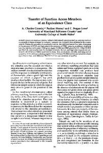
Fig. 1. Representations of a reference circuit and its mutant. nodes have netspan = 1, edges connecting cell nodes and net nodes have netspan = 0. Interchangeably, we may refer to these edges as wires or two-pin nets. Also, we will refer to the set of all edges with netspan = 1 at level i and nodes incident at these edges as the mutation channel at level i. Similarly, we will refer to the set of all edges with netspan = 0 at level i and nodes incident at these edges as the permutation channel at level i. The motivation for these de nitions will become clear later in this section. Acyclic Netlist Model. In this paper, we only consider netlists that are acyclic, where each cell drives only one net, and is driven by one or more nets. The unique characteristics of a netlist that we capture before its transformation into a canonical bipartite directed graph model are the following: (1) all nets not driven by a cell are assigned a level = 0 and designated as primary inputs (PIs); (2) all cells are assigned a level > 0, determined uniquely by the topological sort of the netlist; (3) each pin of the net inherits the level of the incident cell; (4) for each net, netspan > 0, always; (5) a pin of the net not driving a cell is designated as a primary output (PO). An extension of the characterization for netlists with cycles and its canonical form will be presented elsewhere. C-BIDAG Model. The canonical bipartite directed graph model (C-BIDAG) is a transformation of an acyclic netlist. The order of this transformation is important. T1: For each PI net, initially at level = 0, and driving cells at level = ki , re-assign level = minfki g ? 1 since such a PI net does not determine the level of any of the cells it drives. This is due to the cell level topological order assignments. T2: For each net, driven by pin i (at level j ) and netspan = k +1; k > 1, (a) connect net i to input pins of all incident cells at level j + 1, (b) place a single-input, single-output feedthrough cell at level j + 1, connect its input pin to pin i, and connect its output pin to input pins of all incident cells at level j + 2, (c) repeat step (b) x-times until j + x = k + 1. T3: Replace each net with a net node (a net node mirrors the cell node: its fanin is 1 and fanout is variable). A canonical form of the netlist in Figure 1(a) is shown in Figure 1(b). For example, the PI net e has been moved from level 0 to level 1, and the 3-pin net r with netspan of 2 has been transformed into a net node r driving a feedthrough node R.1 which in turn drives a net node r.1. With respect

w

to Figure 1(b), it can be readily veri ed that edges connecting net nodes to cell nodes span levels i ? 1 and i, while edges connecting cell nodes to net nodes remain at level i. Wiring Perturbation Model of C-BIDAG. A wiring perturbation is de ned for both the mutation channel and the permutation channel at level i as de ned earlier. Basically, it amounts to the removal of p wires or q% wires from either or both of the channels at level i; starting at level 1 and completing at the highest level. An example of 60% wiring perturbation is shown in Figure 1(c). For example, at level 1, there are a total of 8 wires in the mutation channel. A 60% perturbation implies a removal of 5 wires. A level-wise distribution of all 60% wiring perturbations in the mutation channels for this circuit is thus f5; 4; 4; 3; 1; 1g. The upper bound on the number of mutants for this perturbation is 288x18x6x9x1x1 = 279,936. Results using 100 randomly selected mutants show a surprising range of variations of optimizing objectives for the algorithms considered { even for such a small reference circuit. Reference Circuit Mutation. A reference circuit mutation is induced by the p-wire or q%-wire perturbation of the reference circuit in C-BIDAG form. The wiring perturbation leaves some of the nodes in the circuit oating and the mutation process consists of restoring, as a random process, all connections that have been removed by the wiring perturbations. An example of a circuit mutant induced by the 60% wiring perturbations in Figure 1(c) is shown in Figure 1(d). The circuit mutant does not look isomorphic to its reference circuit in Figure 1(b). However, it has a number of properties that make it belong to the mutant equivalence class as de ned next. III. Wiring Signature Invariance As demonstrated, introducing edge perturbations and reconnecting the nodes can change the structure of the graph dramatically . The question arises what properties about the graph can be maintained as invariant during this process while still creating a diversity of useful graph mutations. The wiring signature, illustrated in Figure 2, is subject to conditional incidence relationships and bounds on the net node fanout and has the required properties. Wiring Signature. The reference circuit representation in the canonical form as de ned in this paper suggests a circuit signature as a distribution of characteristic cuts in a levelorder. Each characteristic cut is de ned for level i as follows: Li;I : total number of PI net nodes; Li;O : total number of PO net nodes; Li;A : total number of net nodes driven by feedthrough cells; Li;1 : total number of net nodes driven by 1-input combinational cells; Li;2 : total number of net nodes driven by 2-input combinational cells; xi;X : upper (x = max) and lower (x = min) bounds on the total fanout for net nodes of type X , where X = I is the Level i : --------: : : : :

Li;I Li;O Li;A Li;1 Li;2

0 1 2 3 4 5 6 -------------4 1 0 0 0 0 0 0 0 0 0 0 0 1 0 0 1 0 1 1 0 0 0 0 0 0 0 0 0 4 3 3 2 1 1

BASIC SIGNATURE

Level i : --------: : : : : : :

min i;C min i;I min i;A 'min i;C min 'i;I 'min i;A qi+1

0 1 2 3 4 5 6 Level i : 0 1 2 3 4 5 6 -------------- --------- -------------0 3 3 2 2 1 1 : 0 6 5 5 2 1 1 8 1 0 0 0 0 0 : 8 3 0 0 0 0 0 0 0 1 0 1 1 0 : 0 0 3 0 1 1 0 0 1 1 1 1 1 1 : 0 3 3 3 1 1 1 1 1 0 0 0 0 0 : 4 3 0 0 0 0 0 0 0 1 0 1 1 0 : 0 0 3 0 1 1 0 0 8 7 6 5 3 2 SIGNATURE EXTENSION

max i;C max i;I max i;A 'max i;C max 'i;I 'max i;A

Fig. 2. An example of a circuit signature and its extension.

case of a PI net node, X = A is the case of a net node driven by a feedthrough cell, X = C is the case of a net node driven by axcombinational cell; 'i;X : upper (x = max) and lower (x = min) bounds on any single node fanout for net nodes of type X , where X = I is the case of a PI net node, X = A is the case of a net node driven by a feedthrough cell, X = C is the case of a net node driven by a combinational cell; qi+1 : total number of cell input pins at level i + 1 to be driven by net nodes at level i. To keep the size of the signature manageable, we have restricted it to 1- and 2-input combinational cells only. The signature for a general sequential circuit is more complex and will be presented elsewhere. Speci cally, the wiring signature for the reference circuit in Figure 1(b) is shown in Figure 2. We refer to the rst 5 rows on the leftmost column as the `basic signature', and the remainder as the `extended signature'. For example, note that at level 2, the basic signature records the presence of 3 net nodes driven by 2-input cell nodes, and 1 net node driven by a feedthrough cell. While the statistics contained in the `basic signature' may appear trivial at rst glance, they give rise to unique bounds on the fanout of the net nodes shown as a part of the `extended signature'. An example of these bounds will be discussed later in the section. Conditional Incidence Relationships. Restoring the connections after any perturbation of the reference circuit canonical form, including the removal of all wires, may result in a circuit whose wiring signature will be dierent from the one generated for the reference circuit. The canonical form graph imposes a set of unique conditions on how net nodes may drive the cell nodes such that the wiring signature is maintained when reconnecting the edges that have been removed between the net nodes and cell nodes. Table I summarizes all of the conditional incidence relationships of net nodes at level i ? 1 to cell nodes at level i that must be maintained to restore a mutant circuit whose signature will match the signature of the reference circuit under any perturbation. Net Node Fanout Bounds. Given the basic signature, the bounds on the fanouts of each net node are invariant. These are included as a signature extension in Figure 2. For example, at level 2, the minimum fanout on the net nodes of type C is 3 and the maximum is 5. The corresponding values for fanouts on individual net nodes of type C are 1 and 3 respectively. During mutation, the signature is maintained for any choice max of i;X ('i;X ) provided that i;X 2 [min i;X ; i;X ] and 'i;X 2 max ['min i;X ; 'i;X ], X 2 fC; A; I g. As an example, min i;C is given by min i;C = max (Li;1 + Li;2 ; Li+1;2 + Li+1;1 )

(1)

The formulation of min i;C is dictated by the fact that the level of each combinational gate at level i + 1 has to be asserted by an edge from a net node of type C at level i (condition B1 in Table I), and, each net node must drive at least one edge. Maximum number of edges driven by C-type net nodes is given by: ?

1;max 2;max max i;C = min i;C ; i;C




(2)

;max = qi+1 ? Li;I ? Li;A and 2;max = 2  Li+1;2 ? where 1i;C i;C Li;I +min (Li;2 + Li;1 ; Li+1;1 )+min (Li;2 + Li;1 ; Li+1;A ). The complete set of bounds (a total of 12), required to preserve the signature, is omitted. Note that, within the bounds, the reference circuit and the mutant may have a dierent distribution across the dierent types of net nodes. However, all

TABLE I

Conditional incidence relationships for the canonical form.

Cell nodes Net nodes at level i Conditions at level i?1 fta lgb lg-driven 0 1 A1: cannot drive the same node twice lg-driven 1 0 A2: cannot drive more than 1 feedthrough lg-driven 1 1 A3: must satisfy A1 and A2 ft-driven 0 1 B1: level of cell at level i must be asserted by a lg-driven net node at level i?1 ft-driven 1 0 B2: cannot drive more than 1 feedthrough ft-driven 1 1 B3: must satisfy B1 and B2 PO(term.) 0 0 C0: must be lg{driven at level i?1 PO(driving) 0 1 C1: must satisfy C0 PO(driving) 1 0 C2: must satisfy C0 and A2 PO(driving) 1 1 C3: must satisfy C0 and A3 PIc 0 1 D1: must satisfy B1 PI 1 0 D2: must not be allowed PI 1 1 D3: must satisfy B1 and B2 a feedthrough cell nodes b logic cell node c At least one PI node is at level 0

mutants share the same signature extension, i.e. the same fanout bounds, with the reference circuit. Wiring Signature-Invariant Class. Given a topologically sorted acyclic netlist model as de ned in this paper, the wiring signature of its C-BIDAG model is unique. Consider a reference circuit 0 and its wiring signature 0 . A wiring-signature-invariant equivalence class N 0 is the set of all circuits whose wiring signature is 0 . We say that these circuits are mutants of the reference circuit 0 . Speci cally, the mutants are induced by a wiring perturbation and are denoted as  i 2 N 0 . In Section 5, we introduce 8 speci c subclasses (A{H) of the wiring signature invariant mutants. The subclasses are dierentiated by dierent degrees of perturbation ( ). IV. Synthesis of Mutants This section presents a synthesis procedure for any number of circuit mutants. The goal of the synthesis process is to reconnect the removed wires in a perturbed circuit such that the signature of the reference circuit is restored. The synthesis algorithm MUTATE, outlined in this section, relies on the following theorem (proof omitted for brevity). Theorem: Given the basic signature of the reference circuit, any circuit mutant satisfying the fanout bounds of the extended signature will remain in the same equivalence class. Connection Assignments. We consider three connection assignments at level i; i > 0: (A1): bounded net node edge connection (mutation channel). Here, pi net nodes at level i are assigned a bounded distribution of qi+1 edges that are to be connected to qi+1 input pins of cell nodes at level i + 1; (A2): restricted cell node edge connection (mutation channel). Here, qi+1 edges driven by net nodes at level i are connected to qi+1 input pins of cell node at level i + 1, subject to forbidden permutation positions; (A3): unrestricted permutation connection (permutation channel). Here, pi+1 edges driven by cell nodes at level i + 1 drive pi+1 net nodes at level i + 1. This step is well understood. Illustrative Example. We make use of the single mutation channel i in Figure 3 to illustrates the process. (a) The complete signature for the reference channel is f(1; 0; 1; 1; 1); ([3; 5]; [1; 3]; [1; 2]); ([1; 4]; [1; 3]; [1; 2]); 7g. For readability, the signature is shown in four parts:  basic signature;

AA AA AAA AAA AAA AA AA AAAA AA AAA AAA AA AAAA AAA AAAA AA AAA AAA AA AA AAA AA AAA AAA AA AAAA AA AAA AA AAA AAAA AA AAA AAA AA AA AAAA AAA AAA AAAA AAA AA C C I

A

AAA AA AA AAA AAA AA AA AAA AAA AAAA AAAA AAA AAA AAAA AAAA AAAAAAA AAAA AA AAA AA AAAAAAA AAA AA AAA AAA AA AAA AAA AA AAAA AA AAA AA AAA AAA AAAA AA AAA AAA AAAAAAAA AAAA AAAA AAA AA AAAAAAA AA AAA AAAA AA

(a) Reference channel “i”

C C I

A

(d) Step 1 of Assignment A2

C C I

A

AAA AAA AA AAA AAAA AAA AAA AAAA AAAA AAA AAA AAA AA AA AAA AAAAAAA AAA AA AAA AAA AA AAA AA AAA AAA AA AAA AAA AAAA AAAA AAA AAA AA AAA AAAA AA AAA AAA AAA AAAA AAA AAA AAA AA AAAAAAA AA AAA AAA AA C C I

A

AAA AAA AAA

(b) 100% perturbed channel “i” (c) channel “i” after assignment A1

C C I

A

(e) Step 2 of Assignment A2

C C I

A

AAA AAA AAA AAA

((f) Step 3 of Assignment A2

Fig. 3. Single channel mutation sequences.

 extended part of the signature relating to bounds on total

fanout of net nodes of type C, I, A;

 extended part of the signature relating to bounds on in-

dividual fanout of net nodes of type C, I, A;  number of cell input pins to be driven by net nodes at level i. (b) Here we show the case of 100% wiring perturbation. The case of partial perturbation can be presented similarly. (c) This is an illustration of the bounded net node edge connection (Assignment (A1)). According to the signature, the bound on C-type net nodes is [3; 5]. Here, the random choice returns 4 edges. Similarly, the bound on I-type net nodes is [1; 3], and the bound on A-type net nodes is [1; 2]. The random choice returns 2 edges and 1 edge, respectively. Since there are 2 C-type nodes, we need to distribute the 4 C-type edges to individual net nodes such that the fanout on either net node does not exceed the individual fanout bound [1; 4]. Formally, the assignment is always done in the following order : i;C ; i;I ; i;A ; 'i;C ; 'i;I ; 'i;A . (d, e, f) This is an illustration of the restricted cell node edge connection (Assignment (A2)). The following three steps, in the strict order shown, complete all of the perturbed circuit connections.  connect any edge driven by C-type net node to an input pin of a logic node such that condition B1 in Table I is satis ed;  connect any edge driven by I-type net node to an input pin of a logic node whose level has already been asserted by a C-type net node (this step satis es conditions D1, D2, D3 in Table I);  connect all remaining edges driven by any net node type to an input pin of a logic or feedthrough cell node under the constraints of Table I. Pseudo{code of MUTATE. In Figure 4, we show a section of pseudo-code of the MUTATE algorithm, notably the connection assignments A1{A2. Essentially, the mutation process consists of a sequence of connections from net nodes to cell nodes and vice versa. To generate each mutant, the process progresses from level 0 to the highest level. Selection of a speci c pair of fnet nodes, cell nodeg is done by a random choice out of a feasible set that conforms to the constraints in Table I and the fanout bounds such as Eqs. (1{2). Time and Memory Complexity of the Algorithm. The algorithm always works on two adjacent levels and the computations at level i does not depend on any of the results of levels  i ? 2. Hence the process may be described as memoryless. The storage complexity is O(m) where m is the maximum size of all the levels. The time complexity of the

for # of mutants to be generated f for each level i from 0 to max level f do assgn A1; do assgn A2; do assgn A3; g g A1() max f function do assgn min

i;C =rand assgn(i;C = qi+1 ? 
i;C
; ? ; i;C ); remainder ? max i;I =rand assgn min ; i;I ; min i;I ; remainder remainder = remainder ? i;C ; i;A = remainder;

for each net node of type C f

remainder = fanouts ? left in i;C?; max
'i;C =rand assgn 'min i;C ; min 'i;C ; remainder




remainder = fanouts ? left in i;I?; max
'i;I =rand assgn 'min i;I ; min 'i;I ; remainder




remainder = fanouts ? left in i;A?; max
'i;A =rand assgn 'min i;A ; min 'i;A ; remainder




for each net node of type I f

for each net node of type A f

function do assgn A2() f

;

g

;

g

;

gg

f

for each cell node y at i+1 pick x at random from i;C and connect it to y for each net node y of type I at level pick x at random from i+1;2 and connect y to x for each i which is not yet connected calculate feasible set of cell nodes; pick x at random from the feasible set and connect to the net node

g



L

'

if

f

g

gg

Fig. 4. A section of MUTATE pseudo{code algorithm can be stated as O(j V j + j E j)k , where j V j is the number of cell nodes in the circuit and j E j is the number of nets and 1  k  2. V. Design of Experiments The capability to synthesize a large number of WSI circuit mutants, based on wire perturbation classes, motivates us to examine the sampling methods that arise in the design of experiments. Such methods, rst formalized in [5], have been adopted widely in many elds of science. In this paper, we adapt them to analyze the performance of important graphbased algorithms in the context of EDA. For each reference circuit, we propose to synthesize equivalence subclasses of circuit mutants, based on 0 to 100% perturbation. Each subclass contains 100 randomly chosen mutant circuits, each listed in a dierent random order. This sample size is large enough for the sampling distributions to be considered normal or nearly normal; the population parameters may be estimated closely by their corresponding sample statistics. The eight equivalence subclasses, labeled from A to H , are de ned in terms of the perturbations we use to generate each class. In order to encourage unbiased experiments with these classes, we have permuted the perturbations relative to the label assignments:

fA; B; C; D; E; F; G; H g = permutationf0w; 1w; 2w; 5%; 10%; 20%; 40%; 100%g (3) In (3), WSI classes A-H are de ned either in terms of q% wire perturbations or 0-wire, 1-wire, 2-wire (0w; 1w; 2w) perturbations. We plan to identify the labels A-H in terms of the respective perturbation classes in (3) later, once there are additional experiments reported by others and participants have the opportunity to meet and present their results at a joint session of a conference. More details about such plans can be found under http://www.cbl.ncsu.edu/experiments/. A case study tutorial of average-case performance of two algorithms and their dierences has demonstrated that up to six distinct equivalence classes of data are useful to render an unbiased comparison of two well-known sorting algorithms

[6]. The long-term goal of this series of experiments, presently starting with eight equivalence classes, is to facilitate generation of similar comparisons for the more complex and diverse algorithms in EDA. Whatever may be decided about the most suitable number of equivalence classes through wider participation later on, the class of 0-wire perturbations will remain important. As demonstrated in this paper as well as earlier [7], the objective functions used in a number of graph-based algorithms can be very sensitive to the order of nodes in the graph, even when graphs are isomorphic. In our experiments, the 100 netlists in the 0-wire perturbation class are simply isomorphic instances of the reference netlist in a randomized order. Paraphrasing the context of the traditional treatments and blocks [8], we propose to archive data in the context of algorithms and equivalence class mutants as shown in Figure 5(a). For each of the `a' algorithms we consider `b' mutants in one of the equivalence classes in (3). For each algorithm Alg_j and mutant M-X_k, X 2 fA; : : : ; H g, we record two observations: the initial value of the objective function tuple X_jk-I, and the nal value of the objective function tuple X_jk-F. The initial value corresponds to a placebo treatment of the mutant M-X_k: it is the value of the objective function before engaging the algorithm to optimize it. The nal value corresponds to the optimized value of the objective function after engaging the algorithm to optimize it. A number of analyses can be performed once data is archived as shown in Figure 5(a) and only a few are discussed in this paper. For the most part, we shall concentrate on analyzing data as presented in Figure 5(b). In particular, for samples associated with each algorithm Alg_j and mutant class M-X, X 2 fA; : : : ; H g, we evaluate the 95% con dence interval of the sample mean, the sample mean, and the sample variances as tuples {M-X_j-I} and {M-X_j-F} respectively. We summarize such evaluations in the form shown in Figure 5(c). The next section provides representative summaries of data samples we generated and archived under http://www.cbl.ncsu.edu/experiments/. VI. Experiments This section summarizes experiments based on four classes of WSI circuit mutants, based on reference circuits V65E3-64, V65E1-66, C499, and C1355. The rst two reference circuits belong to a family of 2-layer graphs introduced in this paper, the other reference circuits belong to the ISCAS85 set [9] and are also documented in [10]. With eight subclasses AH and 100 mutant circuits in each class, we summarize a total of 14,400 experiments covering representative cases of 13 algorithms. Complete tables of all data samples summarized in this paper have been archived on our web site (http://www.cbl.ncsu.edu/experiments/). The archives are being updated periodically with additional experiments and cases of more detailed statistical analyses [11]. The web site provides an open forum to interested researchers for further sampling, tests of signi cance and hypotheses, and statistical inference of existing data and benchmarks, as well as for contributing new cases of benchmarks, new data of experiments, and new cases of statistical analysis. The site will maintain contributions of participants either as hyperlinks to data and documents on participant's web site, or new archives will be created under http://www.cbl.ncsu.edu/experiments/. In this section we describe brie y the context of the experiments and provide a `textbook' statistical summary of uncorrelated 95% con dence interval of the sample mean, the sample mean and the sample standard deviation. We only brie y allude to some fundamental issues, such as

======================================================== (a) algorithms-vs-mutants-vs-classes ======================================================== M-H_1 .... M-H_k .... M-H_b | ---------------------------------| ................................. | M-B_1 .... M-B_k .... M-B_b | | -----------------------------------| | M-A_1 .... M-A_k .... M-A_b | | | -----------------------------------| | | Alg_1-I A_11-I .... A_1k-I .... A_1b-I | | | Alg_1-F A_11-F .... A_1k-F .... A_1b-F | | | ..... | | | Alg_j-I A_j1-I .... A_jk-I .... A_jb-I | | Alg_j-F A_j1-I .... A_jk-F .... A_jb-F | | ..... | | Alg_a-I A_a1-I .... A_ak-I .... A_ab-I | Alg_a-F A_a1-F .... A_ak-F .... A_ab-F | ======================================================== (b) classes-vs-mutants (for a given algorithm Alg_j) ======================================================== Alg_j-F M-._1 .... M-._k .... M-._b -----------------------------------M-A A_j1-F .... A_jk-F .... A_jb-F {M-A_j-F} M-B B_j1-F .... B_jk-F .... B_jb-F {M-A_j-F} .... M-H H_j1-F .... H_jk-F .... H_jb-F {M-H_j-F} -----------------------------------{M-._j1-F} ..{M-._jk-F} ..{M-._jb-F} ======================================================== (c) statistics of algorithms-vs-mutant classes ======================================================== M-A M-B ..... M-H ---------------------------------Alg_1-I {M-A_1-I} {M-B_1-I} ... {M-H_1-I} Alg_1-F {M-A_1-F} {M-B_1-F} ... {M-H_1-F} ..... Alg_j-I {M-A_j-I} {M-B_j-I} ... {M-H_j-I} Alg_j-F {M-A_j-F} {M-B_j-F} ... {M-H_j-F} ..... Alg_a-I {M-A_a-I} {M-B_a-I} ... {M-H_a-I} Alg_a-F {M-A_a-F} {M-B_a-F} ... {M-H_a-F}

Fig. 5. Data structures and classes for the proposed experiments.  Consider, for a given mutant class, (1) sample mean and

standard deviation of the unoptimized objective function, and (2) sample mean and standard deviation of the objective function optimized via algorithm Alg_j. We have to decide: (H0) is the dierence in the means due to chance, or (H1) is it due to the eect of algorithm Alg_j?  Consider, for a given algorithm Alg_j, (1) sample mean and standard deviation of the optimized objective function in terms of mutant class A, and (2) sample mean and standard deviation of the optimized objective function in terms of mutant class B . We have to decide: (H0) is the dierence in the means due to chance, or (H1) is it due to dierences of the two mutant classes?  Consider, for a given mutant class (1) sample mean and standard deviation of the objective function optimized by algorithm Alg_j1, and (2) sample mean and standard deviation of the objective function optimized by algorithm Alg_j2. We have to decide: (H0) is the dierence in the means due to chance, or (H1) is it due to dierent performances of the algorithms Alg_j1 and Alg_j2? For example:  Upon inspection of initial (DOT I) and nal (DOT F) wire-crossing results in Figure 6, we do not need a t-test to declare that the wire crossing minimization algorithm implemented in DOT [12] is highly eective.

20

25

15

10

5

0

25

Random graphs (V=65,E=131)

30

V65E3-64 Mutants (ClassB)

V65E3-64 Mutants (ClassD)

25

20 15 10 5

5 25 45 65 85 Minimized wire crossing W ClassA

105

W ClassB

15

10

5

0

0