Abstract. String editing problem is one of the most fundamental problems in
computer science ... However it does not address the problem of computing the
edit.
Synthesizable, Space and Time Efficient Algorithms for String Editing Problem. by
Vamsi K. Kundeti B.S.,Indian Institute of Information Technology, Hyderabad,2004
A Thesis Submitted in Partial Fulfillment of the Requirements for the Degree of Master of Science at the University of Connecticut 2008
APPROVAL PAGE
Master of Science Thesis
Synthesizable, Space and Time Efficient Algorithms for String Editing Problem.
Presented by
Vamsi K. Kundeti
Major Advisor: Dr. Sanguthevar Rajasekaran
Associate Advisor: Dr. Ion I. Mandiou
Associate Advisor: Dr. Yufeng Wu
University of Connecticut 2008
ii
Abstract String editing problem is one of the most fundamental problems in computer science and is used extensively in Bio-Informatics. In this thesis we present two new results relevant to the string editing problem. Firstly we show how we can simultaneously compute both the edit distance and edit script between two strings of length n in time O(n2 /log(n)) and O(n) space. The Four Russian algorithm computes the edit distance in time O(n2 /log(n)). However it does not address the problem of computing the edit script. On the other hand Hirschberg’s algorithm computes the edit script in O(n) space but takes O(n2 ) time. In this thesis we show how to compute both the edit distance and edit script within the best known time and space bounds. Secondly we provide a new algorithm which can be readily synthesized into an area efficient and high speed sequential digital circuit to compute the edit distance in hardware at a clock speed of 1 GHz. The simplicity of the design makes it possible to add this to any general purpose processor instruction set. An instruction from the processor to compute the edit distance between constant length strings can clearly aid in improving the performance of the software. Our experiments estimate a 4X speedup from a processor with a 8 × 8 edit distance instruction. 1. V.K. Kundeti and S.Rajasekaran. ”Extending The Four Russian Algorithm to Compute the Edit Script in Linear Space.”, (Springer LNCS 5101-0893) ICCS2008, Krakow, Poland. 2. V.K. Kundeti , Y.Fei. and S.Rajasekaran ”An Efficient Digital Circuit for Implementing Sequence Alignment Algorithm in an Extended Processor.”,19th IEEE ASAP-2008, Leuven, Belgium.
iii
Contents Abstract
iii
1 Introduction
1
1.1
Problem Definition . . . . . . . . . . . . . . . . . . . . . . . . . . . . . . .
1
1.2
Applications of the edit distance based algorithms . . . . . . . . . . . . .
2
1.3
Dynamic programming formulation for the edit distance Problem . . . . .
3
1.4
Analysis of the standard algorithm for edit distance . . . . . . . . . . . .
5
2 Space and Time Efficient Algorithms for Computing Edit Distance
7
2.1
Related work . . . . . . . . . . . . . . . . . . . . . . . . . . . . . . . . . .
8
2.2
Four Russian Algorithm . . . . . . . . . . . . . . . . . . . . . . . . . . . .
9
2.2.1
Pre Processing Step . . . . . . . . . . . . . . . . . . . . . . . . . .
12
2.2.2
Computation Step . . . . . . . . . . . . . . . . . . . . . . . . . . .
13
2.3
Hirschberg’s Algorithm to Compute the Edit Script . . . . . . . . . . . . .
13
2.4
Our Algorithm . . . . . . . . . . . . . . . . . . . . . . . . . . . . . . . . .
15
2.5
Space Complexity . . . . . . . . . . . . . . . . . . . . . . . . . . . . . . . .
18
2.5.1
Space During The Execution . . . . . . . . . . . . . . . . . . . . .
18
2.5.2
Space For Storing Lookup Table F . . . . . . . . . . . . . . . . . .
18
Conclusion . . . . . . . . . . . . . . . . . . . . . . . . . . . . . . . . . . .
18
2.6
3 Synthesizable and Area Efficeint Algorithms for Edit Distance 3.0.1 3.1
20
Related Work . . . . . . . . . . . . . . . . . . . . . . . . . . . . . .
21
Hardware Implementation of the EditDistance Algorithm . . . . . . . . . .
22
3.1.1
Storage Block AlgoShifter . . . . . . . . . . . . . . . . . . . . . . .
23
3.1.2
Computation Block ComputeBlock . . . . . . . . . . . . . . . . . .
26
iv
3.1.3
Character Block StringRegister . . . . . . . . . . . . . . . . . . . .
26
3.1.4
Control Block CounterBlock . . . . . . . . . . . . . . . . . . . . . .
27
3.2
Using EditDistance Instruction in an Extensible Processor . . . . . . . . .
27
3.3
Verification and Experiments . . . . . . . . . . . . . . . . . . . . . . . . .
28
3.3.1
Speed-up Estimation with Hardware Implementation . . . . . . . .
30
3.4
RTL Code and Details on Usage . . . . . . . . . . . . . . . . . . . . . . .
31
3.5
Conclusions . . . . . . . . . . . . . . . . . . . . . . . . . . . . . . . . . . .
32
v
List of Figures 1.1
Illustration of edit distance optimization problem . . . . . . . . . . . . . .
2
1.2
Illustration of the flow of edit distance computation . . . . . . . . . . . .
4
2.1
Using preprocessed lookup table {A′ , B ′ , K ′ } = F (A, B, C, K, E). . . . . .
11
2.2
Illustration of Hirschberg’s recursive algorithm. . . . . . . . . . . . . . . .
14
3.1
Top-level block diagram of the circuit . . . . . . . . . . . . . . . . . . . .
23
3.2
Internal details of block AlgoShifter . . . . . . . . . . . . . . . . . . . . . .
24
3.3
Operation of the shift register in first clock cycle . . . . . . . . . . . . . .
25
3.4
Internal details of ComputeBlock . . . . . . . . . . . . . . . . . . . . . . .
26
3.5
Internal Details of StringRegister . . . . . . . . . . . . . . . . . . . . . . .
27
3.6
Internal details of CounterBlock . . . . . . . . . . . . . . . . . . . . . . . .
28
3.7
Illustration of the first two steps of Edit Distance computation with the
3.8
EditDistance instruction from an extended processor . . . . . . . . . . . .
29
Simulation waveforms for S1 = [aaaabcda], S2 = [aaabcada] . . . . . . . .
33
List of Algorithms 1.1 EditDistance . . . . . . . . . . . . . . . . . . . . . . . . . . . . . . . . . . . . . .
5
2.2 FourRussianAlgo . . . . . . . . . . . . . . . . . . . . . . . . . . . . . . . . . . . .
9
2.3 LookUp . . . . . . . . . . . . . . . . . . . . . . . . . . . . . . . . . . . . . . . .
11
2.4 TopLevel . . . . . . . . . . . . . . . . . . . . . . . . . . . . . . . . . . . . . . . .
16
2.5 FindScript . . . . . . . . . . . . . . . . . . . . . . . . . . . . . . . . . . . . . . .
17
vi
2.6 FourCompute . . . . . . . . . . . . . . . . . . . . . . . . . . . . . . . . . . . . .
19
3.7 EditDistanceInstruction . . . . . . . . . . . . . . . . . . . . . . . . . . . . . . . .
29
List of Tables 3.1
Comparision of various design metrics with Clock Period(T)
. . . . . . .
30
3.2
Estimated cycles required with various hardware implementations . . . . .
30
vii
Chapter 1
Introduction Computing the edit distance between two strings is one of the most fundamental problem in computer science [CLRS01]. Assume we have two strings, S1 = [a1 , a2 , a3 , . . . , an ] and S2 = [b1 , b2 , b3 , . . . , bm ], and a set of operations {Insert(I), Delete(D), Change(C)}, each of the operations I, D, C can be applied to the characters in the strings at a given position. For example, if S1 = [aaaabcda] and S2 = [aaabcada], applying an operation D to the string S1 at position 8 (the rightmost character) changes it to [aaaabcd ], applying an operation I(x) to S2 at position 8 inserts a character x to S2 and changes it to [aaabcadxa], and applying an operation C(b) to S1 at position 4 which has a character a makes it [aaabbcda] by changing the character from a to b. Note that all the operations need the position specified, and I and C need an additional character for replacement. Figure 1 illustrates a simple example on the motivation behind the edit distance problem.
1.1
Problem Definition
The edit distance problem asks for a set of operations with minimum cost required to transform string S1 to S2 (or S2 to S1 ), with each of the operations associated with a cost. In this thesis, we consider a simplified problem, where each of these operations (I, D, C) has a unit cost, and hence minimizing the number of operations is equivalent to minimizing the cost. We consider the previous example with S1 = [aaaabcda], S2 = [aaabcada], and we can transform S1 to S2 by a sequence of operations as follows: change character a at position 4, b at position 5, and c at position 6 of S1 to b, c and a, respectively, by operations C(b), C(c), and C(a). We can describe the series of operations as a transcript T = {−, −, −, C(b), C(c), C(a), −, −}, where − at positions 1, 2, 3, 7, 8 1
AAAABCDA
AAABCADA
What is the best way to align ? COST = 2 S1 S2
COST = 3
AAAABCADA AAAXBCADA Delete in Insert in
S1
AAA A B C DA AAA B C A DA
Change in
S1
S1
Figure 1.1: Illustration of edit distance optimization problem indicates no-operation, and the 3 operations at positions 4, 5, 6 result in a cost of 3 units. ′
However, we can also transform S1 to S2 by applying the following transcript T to S1 , ′
T = {−, −, −, D, −, −, I(a), −, −}, where operation D deletes the character at position ′
4 of S1 , and operation I(a) inserts a character a at position 7 in S1 . T requires only 2 operations whereas T requires 3 operations. The edit distance problem asks to find the minimum number of operations which can transform S1 to S2 . The general edit distance problem can have different costs for each of the operations, all our algorithms can be directly extended for the general model although we work with the unit cost model.
1.2
Applications of the edit distance based algorithms
Algorithms based on edit distance have several applications, a practical example of edit distance in our day to day work is the UNIX diff utility. The UNIX diff utility takes two text files and tells us to convert one file to the other with minimum edit operations (inserting a line, deleting a line, changing a line). Edit distance based algorithms are also used extensively in Bio-Informatics and Computational Genomics. The first application of the edit distance algorithm for protein sequences alignment was studied by Needleman [NW70]. Sequence Alignment is used extensively by biologists to identify similarities between genes of different species, with genes being characterized by DNA sequence, e.g., Sdna = [c1 , c2 , c3 , . . .], ci ∈ A, T, G, C, where A, T , G, and C are symbols for amino acids 2
(also called base pairs). Biologists often analyze the functionality of newly discovered genes by comparing them to genes which were already discovered and whose function is new and S known , biologists perform a sequence fully known. Given two DNA sequences, Sdna dna
alignment (EditDistance computation) between the two sequences to find if they have the same functionality. If the EditDistance value between two genes is below a threshold, both the DNA sequences have some properties in common; otherwise they differ. These DNA sequences are very long, typically running into millions of base pairs. The ever increasing volume of the genomic sequences demand for highly efficient algorithms to help biologists to perform faster sequence alignments. The first algorithm to perform sequence alignment was given by Needleman [NW70] which is a directly based on edit distance computation. Later algorithms for several variations (such as local alignment, affine gap costs, etc.) of the problem were developed (for example) in [SW81], [Got86], and [HHM90].
1.3
Dynamic programming formulation for the edit distance Problem
Dynamic Programming is a general algorithmic framework which can be applied to solve optimization problems which have independent sub problems. The edit distance problem is widely used to illstrate the ideas behind dynamic programming. Any algorithm based on dynamic programming will need to define a sub problem with variables capturing all the details of the optimization problem. The following dynamic programming formulation is the key to the edit distance algorithm. S1 = [a1 , a2 , a3 . . . an ] S1,i = [a1 , a2 . . . ai ] S2 = [b1 , b2 , b3 . . . bn ] S2,j = [b1 , b2 . . . bj ] S1,i ,S2,j are prefixes of strings S1 ,S2 D(i, j) =
�
Optimal cost of transforming S1,i to S2,j
3
Initialization of dynamic programming D(i, 0) = i Cost aligning [a1 , a2 . . . ai ] with empty string D(0, j) = j Cost aligning [b1 , b2 . . . bj ] with empty string for 1 ≤ i, j ≤ n, D(i, j) can be computed � as follows 0 If ai = bj D(i − 1, j − 1)+ chg Else D(i − 1, j) + del delete ai and align D(i, j) = min [a1 , a2 . . . ai−1 ] and [b1 , b2 . . . bj ] D(i, j − 1) + ins insert bj and align [a1 , a2 . . . ai ] and [b1 , b2 . . . bj−1 ]
Algorithm 1(EditDistance) demonstrates the pseudo-code the above dynamic program-
a aa ab c d a a a a b c a d a
012345678 101234567 210123456 321112345 432221234 543232223 654333233 765444323 876555432
Figure 1.2: Illustration of the flow of edit distance computation ming formulation. We can think of the sub-problem D(i, j) as a cell in a n × n table (Dn×n ), D(i, j) is the edit distance from the first i characters of S1 to the first j characters of S2 , and D(n, n) is the minimum number of operations to transform S1 to S2 . See Figure 1.2 for the flow of edit distance computation in the table Dn×n . The first step is initialization, giving the edit distance between a NULL string and a prefix of S2 (D(0, j) = j), and also a prefix of S1 and a NULL string (D(i, 0) = i). The computation of other table elements is performed by two loops which output the value of D(i, j) (1 ≤ i ≤ n,1 ≤ j ≤ n) for the two sub-strings, S1,i and S2,j . D(i, j) comes from the minimum one of three costs: D(i-1,j-1)+change cost for changing the ith character 4
of S1,i when the first i − 1 characters of S1,i have been successfully transformed to the first j − 1 characters in S2,j , D(i,j-1)+insert cost for inserting the last character when the first i characters of S1,i transformed to the first j − 1 characters of S2,j , and D(i1,j)+delete cost for deleting ith character of S1,i when the first i − 1 characters of S1,i have been transformed to the first j characters of S2,j . Note that the insert cost and delete cost are both constant unit cost, and the change cost is conditionally determined by the last characters of the two sub-strings - only when they are different, there is need for a change operation. Algorithm 1: Pseudo-code for the algorithm of EditDistance INPUT : Strings S1 and S2 each of length n OUTPUT: Minimum number of operations to transform S1 to S2 /*Initialization*/ for i = 1 to n do D(0, i) = i ; D(i, 0) = i ; end /*Recursive Computation of the Distance Table D*/ for i = 1 to n do for j = 1 to n do change cost = 0; if S1 [i] 6= S2 [j] then change cost = 1; end D(i, j) = M IN (D(i − 1, j − 1) + change cost, D(i, j − 1) + 1, D(i − 1, j) + 1) ; end end return D(n, n) ; Algorithm 1. EditDistance
1.4
Analysis of the standard algorithm for edit distance
We can clearly see from Algorithm 1 this standard dynamic programming algorithm need O(n2 ) time to compute the value of the edit distance between two strings each of length n. Coming to the space requirements of the algorithm to compute a sub problem D(i, j) in the the table Dn×n we need to keep track only previous row D(i − 1, ∗) and the current row which is getting compute i.e D(i, ∗). So if we just need the edit distance value between the two strings we need not keep track of the entire table, its enough to 5
just keep only the current row(during computation) and the previous row, this makes the space complexity of just computing the edit distance value as O(n). But in many contexts we need the actual edit script(sequence of operations which can transform one string to the other) rather than the edit distance value. A straight forward algorithm to get the edit script would need to keep the entire table (Dn×n in the memory to trace back the path from D(n, n) to D(0, 0) which gives the required edit script. Since we keep the entire table in the memory to compute the edit script the space complexity of the algorithm is O(n2 ). In the next chapter we will see how we can reduce this space complexity from O(n2 ) to O(n).
6
Chapter 2
Space and Time Efficient Algorithms for Computing Edit Distance As demonstrated in Chapter 1 the standard dynamic programming-based algorithm takes O(n2 ) time to compute the edit distance of two strings of length n, and O(n2 ) space to compute the actual edit script (i.e., a sequence of Inserts, deletes, and changes that transfroms S1 to S2 ). Often the edit script is more important for several problems (such as sequence alignment) than the value of the edit distance. The first major improvement in the asymptotic runtime for computing the value of the edit distance was acheived in [ADKF70]. This algorithm is widely known as the Four Russian Algorithm and it improves the running time by a factor of O(log n) (with a run time of O(n2 / log n)) to compute just the value of the edit distance. It does not address the problem of computing the actual edit script, which is of wider interest rather than just the value. Hirschberg [Hir75] has given an algorithm that computes the actual script in O(n2 ) time. In paper [RA04] linear space parallel algorithms for the sequence alignment problem were given, however they assume that O(n2 ) is the optimal asymptotic complexity of the sequential algorithm. In this chapter we present algorithms that compute both the edit script and 2
n value in O( log n ) time using O(n) space.
The first major improvement in the asymptotic runtime for computing the value of the edit distance was achieved in [ADKF70]. This algorithm is widely known as the Four Russian Algorithm and it improves the running time by a factor of O(log n) (with a run time of O(n2 / log n)) to compute just the value of the edit distance. It does not
7
address the problem of computing the actual edit script, which is of wider interest rather than just the value. Hirschberg [Hir75] has given an algorithm that computes the actual script in O(n2 ) time and O(n) space. The space saving idea from [Hir75] was applied to biological problems in [Got87] and [MM88]. However the asymptotic complexity of the core algorithm in each of these remained O(n2 ). Also, parallel algorithms for the edit distance problem and its application to sequence alignment of biological sequences were studied extensively (for example) in [EW87] and [RS90].
2.1
Related work
The first major improvement in the asymptotic runtime for computing the value of the edit distance was achieved in [ADKF70]. This algorithm is widely known as the Four Russian Algorithm and it improves the running time by a factor of O(log n) (with a run time of O(n2 / log n)) to compute just the value of the edit distance. It does not address the problem of computing the actual edit script, which is of wider interest rather than just the value. Hirschberg [Hir75] has given an algorithm that computes the actual script in O(n2 ) time and O(n) space. The space saving idea from [Hir75] was applied to biological problems in [Got87] and [MM88]. However the asymptotic complexity of the core algorithm in each of these remained O(n2 ). Also, parallel algorithms for the edit distance problem and its application to sequence alignment of biological sequences were studied extensively (for example) in [EW87] and [RS90]. In paper [RA04] linear space parallel algorithms for the sequence alignment problem were given, however they assume that O(n2 ) is the optimal asymptotic complexity of the sequential algorithm. Please refer to [Gus97] for an excellent survey on all these algorithms. A special case is one where each of these operations is of unit cost. Edit Script is the actual sequence of operations that converts S1 into S2 . In particular, the edit script is a sequence Escript = {X1 , X2 , X3 . . . Xn }, Xi ∈ I, D, C. Standard dynamic programming based algorithms solve both the distance version and the script version in O(n2 ) time and O(n2 ) space. The main result of this chapter is an algorithm for computing the edit distance and edit � 2 � n script in O log n time and O(n) space. The rest of the chapter is organized as follows. In Sec. 2.2 we provide a summary of
8
the four Russian algorithm [ADKF70]. In Sec. 2.3 we discuss the O(n2 ) time algorithm that consumes O(n) space and finally in Sec. 2.4 we show how to compute the edit 2
n distance and script using O( log n ) time and O(n) space.
2.2
Four Russian Algorithm
In this section we summarize the Four Russian Algorithm. Let D be the dynamic programming table that is filled during the edit distance algorithm. The standard edit distance algorithm fills this table D row by row after initialization of the first row and the first column. Without loss of generality, throughout this chapter we assume that all the edit operations cost unit time each. The basic idea behind the Four Russian Algorithm is to partition the dynamic programming table D into small blocks each of width and height equal to t where t is a parameter to be fixed in the analysis. Each such block is called a t-block. The dynamic programming table is divided into t-blocks such that any two adjacent t-blocks overlap by either a row or column of width (or height) equal to t. See Fig. 2.1 for more details on how the dynamic programming table D is partitioned. After this partitioning is done The Four Russian algorithm fills up the table D block by block. Algorithm 2 has more details. Algorithm 2: Four Russian Algorithm, t is a parameter to be fixed. INPUT : Strings S1 and S2 , Σ, t OUTPUT: Optimal Edit distance /*Pre-processing step*/ F = PreProcess(Σ, t) ; for i = 0;i < n;i+ = t do for j = 0;j < n;j+ = t do {A′ , B ′ , D′ } = LookU pF (i, j, t) ; [D[i + t, j] . . . D[i + t, j + t] = A′ ; [D[i, j + t] . . . D[i + t, j + t] = B ′ ; end end Algorithm 2. FourRussianAlgo A quick qualitative analysis of the algorithm is as follows. After the partitioning of the dynamic programming table D into t-blocks we have
n2 t2
blocks and if processing of 2
each of the block takes O(t) time then the running time is O( nt ). In the case of standard dynamic programming, entries are filled one at a time (rather than one block at a time). 9
Each entry can be filled in O(1) time and hence the total run time is O(n2 ). In the Four Russian algorithm, there are
n2 t2
blocks. In order to be able to fill each block in O(t)
time, some preprocessing is done. Theorem 1 is the basis of the preprocessing. Theorem 1 If D is the edit distance table then |D[i, j] − D[i + 1, j]| ≤ 1, and |D[i, j] − D[i, j + 1]| ≤ 1∀(0 ≤ i, j ≤ n).
Proof.
Note that D[i, j] is defined as the minimum cost of converting S1 [1 : i] into
S2 [1 : j]. Every element of the table D[i, j] is filled based on the values from D[i − 1, j − 1],D[i − 1, j] or D[i, j − 1]. D[i, j] ≥ D[i − 1, j − 1](characters at S1 [i] and S2 [j] may be same or different), D[i, j] ≤ D[i, j − 1] + 1 (cost of insert is unity),D[i, j − 1] ≤ D[i − 1, j − 1] + 1(same inequality as the previous one rewritten for element D[i, j − 1]). The following inequalities can be derived from the previous inequalities. −D[i, j] ≤ −D[i − 1, j − 1] D[i, j − 1] ≤ D[i − 1, j − 1] + 1 −D[i, j] + D[i, j − 1] ≤ 1 D[i, j − 1] − D[i, j] ≤ 1 D[i, j] ≤ D[i, j − 1] + 1 {Started with this} −1 ≥ D[i, j − 1] − D[i, j] |D[i, j − 1] − D[i, j]| ≤ 1 Along the same lines we can also prove that |D[i − 1, j] − D[i, j]| ≤ 1 and D[i − 1, j − 1] ≤ D[i, j]. � Theorem 1 essentially states that the value of the edit distance in the dynamic programming table D will either increase by 1 or decrease by 1 or remain the same compared to the previous element in any row or a column of D. Theorem 1 helps us in encoding any row or column of D with a vector of 0, 1, −. For example a row in the edit distance table D[i, ∗] = [k, k + 1, k, k, k − 1, k − 2, k − 1] can be encoded with a vector vi = [0, 1, −1, 0, −1, −1, 1]. To characterize any row or column we just need the vector vi and k corresponding to that particular row or column. For example, if D[i, ∗] = [1, 2, 3, 4, . . . , n], then k = 1 for this row and vi = [0, 1, 1, 1, 1, 1, 1, . . . , 1]. For the computation of the edit distance table D the leftmost column and the topmost 10
S1 S2
11111 00000 E 00000 11111 {A’,B’,K’} = F(A,B,C,K,E)
11 00 00 11 00 11 00 11 00 11 00 11 00 11 C 00 11 00 11 00 11 00 11 00 11 00 11
000 111 0000000 1111111 11 00 B 000 111 0000000 1111111 00 11 00 11 A A’ 00 11 00 11 0000000 1111111 00 11 0000000 1111111 B’ 0000000 1111111 00 11
K
t−block
overlapping row
K’
overlapping column
filled pattern indicates initialized values of the dynamic programming table
Figure 2.1: Using preprocessed lookup table {A′ , B ′ , K ′ } = F (A, B, C, K, E). row must be filled (or initialized) before the start of the algorithm. Similarly in this algorithm we need the topmost row (A) and leftmost column (B) to compute the edit distance within the t-block see Fig. 2.1. Also see Algorithm 3. It is essential that we compute the edit distance within any t-block in constant time. Algorithm 3: LookUp routine used by Algorithm 2. INPUT : i,j,t OUTPUT: A′ , B ′ , D′ A = [D[i, j] . . . D[i, j + t]]; B = [D[i, j] . . . D[i + t, j]]; C = [S2 [j] . . . S2 [j + t]]; E = [S1 [j] . . . S1 [j + t]]; K = D[i, j]; /*Encode A,B*/ for k = 1;k < t;k + + do A[k] = A[k] − A[k − 1]; B[k] = B[k] − B[k − 1]; end /*Although K is not used in building lookup table F we maintain the consistency with Fig. 2.1 */ return {A′ , B ′ , D′ } = F (A, B, C, K, E) ; Algorithm 3. LookUp In the Four Russian algorithm the computation of each t-block depends on the vari-
11
ables A, B, K, C, E (see Fig. 2.1). The variable A represents the top row of the t-block and B represents the the left column of the t-block. C and E represent the corresponding substrings in the strings S1 and S2 . K is the intersection of A and B. If the value of the variable K is k then from Theorem 1 we can represent A and B as vectors of {0,1,-1} rather than with exact values along the row and column. As an example, consider the first t-block which is the intersection of the first t rows and the first t columns of D. For this t-block the variables {A, B, K, C, E} have the following values: K = D[0, 0], A = D[0, ∗] = [0, 1, 1, 1, . . . , 1], B = D[∗, 0] = [0, 1, 1, 1, . . . , 1], C = S2 [0, 1, . . . , t], and E = S1 [0, 1, . . . , t]. For any t-block we have to compute {A′ , B ′ , K ′ } as a function of {A, K, B, C, E} in O(1) time. In this example plugging in {A, B, K, C, E} for the first t-block gives K ′ = D[t, t], A′ = [D[0, t], . . . , D[t, t]],B ′ = [D[t, 0], . . . , D[t, t]]. To accomplish the task of computing the edit distance in a t-block in O(1) time, we precompute all the possible inputs in terms of variables {A, B, 0, C, E}. We don’t have to consider all possible values of K since if K1′ is the value of K ′ we get with input variables {A, B, 0, C, E} then the value of K ′ for inputs {A, B, K, C, E} would be K1′ + K. Thus this encoding(and some preprocessing) helps us in the computation of the edit distance of the t-block in O(1) time. The algorithm is divided into two parts pre-processing step and actual computation.
2.2.1
Pre Processing Step
As we can see from the previous description, at any stage of the Algorithm 2 (FourRussianAlgo)we need to do a lookup for the edit distance of any t-block and as a result get the row and column for the adjacent t-blocks. From Theorem 1 its evident that any input {A, B, K, C, E} (see Fig. 2.1) to the t-block can be transformed into vectors of {−1, 0, 1}. In the preprocessing stage we try out all possible inputs to the t-block and compute the corresponding output row and column ({A′ , B ′ , K ′ } (see Fig. 2.1). More formally, the row (A′ ) and column(B ′ ) that need to be for any t-block can be repesented as a function F (lookup table) with inputs {A, B, K, C, E}, such that {A′ , B ′ , K ′ } = F (A, B, K, C, E). This function can be precomputed since we have only limited possibilities. For any given t, we can have 3t vectors corresponding to A and B. For a given alphabet of size Σ we have Σt possible inputs corresponding to C and E. 12
K will not have any effect since we just have to add K to A′ [t] or B ′ [t] at the end to compute K ′ . The time to preprocess is thus O((3Σ)2t t2 ) and the space for the lookup table F would be O((3Σ)2t t). Since t2 ≤ (3Σ)t , if we pick t =
log n 3 log(3Σ) ,
the preprocessing
time as well as the space for the lookup table will be O(n). Here we make use of the fact that the word length of the computer is Θ(log n). This in particular means that a vector of length t can be thought of as one word.
2.2.2
Computation Step
Once the preprocessing is completed in O(n) time, the main computation step proceedes scanning the t-blocks row by row and filling up the dynamic programming table(D). Algorithm 2 calls Algorithm 3 in the inner most for loop. Algorithm 3 takes O(t) time to endcode the actual values in D and calls the function F which takes O(1) time and returns the row (A′ ) and column (B ′ ) which are used as input for other t-blocks. The 2
runtime of the entire algorithm is O( nt nt t) = O( nt ). Since t = Θ(log n) the run time of 2
n the Four Russian Algorithm is O( log n ).
2.3
Hirschberg’s Algorithm to Compute the Edit Script
In this section we briefly describe Hirschberg’s [Hir75] algorithm that computes the edit script in O(n2 ) time using O(n) space. The key idea behind this algorithm is an appropriate formulation of the dynamic programming paradigm. We make some definitions before giving details on the algorithm. • Let S1 and S2 be strings with |S1 | = m and |S2 | = n. A substring from index i to j in a string S is denoted as S[i . . . j]. • If S is a string then S r denotes the reverse of the string. • Let D(i, j) stand for the optimal edit distance between S1 [1 . . . i] and S2 [1 . . . j]. • Let Dr (i, j) be the optimal edit distance between S1r [1 . . . i] and S2r [1 . . . j]. Lemma 1 D(m, n) = min0≤k≤m {D[ n2 , k] + Dr [ n2 , m − k]}. The Lemma 1 essentially says that finding the optimal value of the edit distance between strings S1 and S2 can be done as follows: Split S1 into two parts (p11 and p12 ) and S2 13
S1 S2
m−k D sub−problem n/2 −1
k
(k at which D[n/2,k]+ Dr [n/2,m−k] is min)
n/2 n/2 −1
subpaths
Dr sub−problem
S r2 S r1
Figure 2.2: Illustration of Hirschberg’s recursive algorithm. into two parts (p21 and p22 ); Find the edit distance (e1 ) between p11 and p21 ; Find the edit distance (e2 ) between p12 and p22 ; Finally add both the distances to get the final edit distance (e1 + e2 ); Since we are looking for the minimum edit distance we have to find a breaking point (k) that minimizes the value of (e1 + e2 ). We would not miss this minimum even if we break one of the strings deterministically and find the corresponding breaking point in the other string. As a result of this we keep the place where we break in one of the strings fixed. (Say we always break one of the strings in the middle). Then we find a breaking point in the other string that will give us minimum value of (e1 + e2 ). The k in Lemma 1 can be found in O(mn) time and O(m) space for the following reasons. To find the k at any stage we need two rows(D[ n2 , ∗] and Dr [ n2 , ∗]) from forward and reverse dynamic programming tables. Since the values in any row of the dynamic programming table just depend on the previous row, we just have to keep track of the previous row while computing the table D and Dr . Once we find k we can also determine the path from the previous row ( n2 − 1) to row ( n2 ) in both the dynamic programming tables D and Dr (see Fig. 2.2). Once we find these subpaths we can continue to do the same for the two subproblems (see Fig. 2.2) and continue recursively. The run time of
14
the algorithm can be computed by the following reccurence relation. T (n, m) = T ( n2 , k) + T ( n2 , m − k) + mn mn T ( n2 , k) + T ( n2 , m − k) = mn 2 + 4 + . . . = O(mn) In each stage we use only O(m) space and hence the space complexity is linear.
2.4
Our Algorithm
Our algorithm combines the frameworks of the Four Russian algorithm and that of � 2 � n time using Hirschberg’s Algorithm. Our algorithms finds the edit script in O log n linear space. We extend the Four Russian algorithm to accommodate Lemma 1 and to compute the edit script in O(n) space. At the top-level of our algorithm we use a dynamic programming formulation similar to that of Hirschberg. Our algorithm is recursive and in each stage of the algorithm we compute k and also find the sub-path as follows. n n D(m, n) = min0≤k≤m {D( , k) + Dr ( , m − k)} 2 2 The key question here is how to use the Four Russian framework in the computation of D( n2 , k) and Dr ( n2 , m − k) for any k in time better than O(n2 )? . Hirschberg’s algorithm needs the rows D( n2 , ∗) and Dr ( n2 , ∗) at any stage of the recursion. In Hirschberg’s algorithm at recursive stage (R(m, n)), D( n2 , k) and Dr ( n2 , m−k) are computed in O(mn) time. We cannot use the same approach since the run time will be Ω(n2 ). We have to find 2
n a way to compute the rows D( nn , ∗) and Dr ( n2 , ∗) with a run time of O( log n ). The top-level
outline of our algorithm is illustrated by the pseudo-code in TopLevel (see Algorithm 4). The algorithm starts with input strings S1 and S2 of length m and n, respectively. At this level the algorithm applies Lemma 1 and finds k. Since the algorithm requires D( n2 , ∗) and Dr ( n2 , ∗) at this level it calls the algorithm FourCompute to compute the rows D( n2 , ∗), D( n2 − 1, ∗), Dr ( n2 , ∗) and Dr ( n2 − 1, ∗). Note the fact that although for finding k we require rows D( n2 , ∗) and Dr ( n2 , ∗), to compute the actual edit script we require rows D( n2 − 1, ∗) and Dr ( n2 − 1, ∗). Also note that these are passed to algorithm FindEditScript to report the edit script around index k.
15
Algorithm 4: TopLevel which calls FourCompute at each recursive level. Input: Strings S1 ,S2 ,|S1 | = m,|S2 | = n Output: Edit Distance and Edit Script D( n2 , ∗) = FourCompute( n2 , m, S1 , S2 , D(∗, 0), D(0, ∗)); Dr ( n2 , ∗) = FourCompute( n2 , m, S1r , S2r , Dr (∗, 0), Dr (0, ∗)); /*Find the k which gives min Edit Distance at this level*/ M inimum = (m + n) ; for i = 0 to n do if (D( n2 , i) + Dr ( n2 , m − i)) < M inimum then k=i; M inimum = D( n2 , i) + Dr ( n2 , m − i) ; end end /*Compute The EditScripts at this level */ k1 = FindEditScript(D( n2 , ∗), D( n2 − 1, ∗), k, F orward) ; k2 = FindEditScript(Dr ( n2 , ∗), Dr ( n2 − 1, ∗), k, Backward) ; /*Make a recursive call If necessary*/ ; TopLevel(S1 [1 . . . k1 − 1],S2 [1 . . . n2 − 1]) ; TopLevel(S1 [m − k2 + 1 . . . m],S2 [ n2 + 1 . . . n]) ; Algorithm 4. TopLevel Once the algorithm finds the appropriate k for which the edit distance would be minimum at this stage, it divides the problem into two sub problems (see Fig. 2.2) (S1 [1 . . . k1 − 1], S2 [1 . . . n2 − 1]) and (S1 [m − k2 + 1 . . . m], S2 [ n2 + 1 . . . n]. Observe that k1 and k2 are returned by FindEditScript(see the pseudo-code of FindEditScript in Algorithm 5 for details). FindEditScript is trying to find if the sub-path passes through the row
n 2
(at
the corresponding level of recursion) and updates k so that we can create sub-problems (please see arcs (sub-paths) in Fig. 2.2). Once the sub-problems are properly updated the algorithm solves each of these problems recursively. We now describe algorithm FourCompute which finds the rows D( n2 , ∗) and Dr ( n2 , ∗) (that are required at each recursive stage of TopLevel (Algorithm 4)) in time O( nm t ) where t is the size of blocks used in the Four Russian Algorithm. We do exactly the same pre-processing done by the Four Russian Algorithm and create the lookup table F . FourCompute is called for both forward (S1 ,S2 ) and reverse strings (S1r ,S2r ). The lookup table F (A, B, K, C, E) has been created for all the strings from Σ of length t. We can use the same lookup table F for all the calls to FourCompute. A very important fact to remember is that in the Four Russian algorithm whenever a lookup call is made to F the outputs {A′ , B ′ } are always aligned at the rows which are multiples of t, i.e., at any stage of the Four Russian algorithm we
16
only require the values of the rows D(i, ∗) such that i mod t = 0. In our case we cannot directly use the Four Russian Algorithm in algorithm FourCompute because the lengths of the strings which are passed to FourCompute from each recursive level of TopLevel is not necessarily a multiple of t. Suppose that in some stage of the FourCompute algorithm a row i is not a multiple of t. We apply the Four Russian Algorithm and compute till row D(⌊ ti ⌋, ∗), find the values in the row D(⌊ ti ⌋ − t, ∗) and apply lookups for rows ⌊ ti ⌋ − t, ⌊ ti ⌋ − t + 1, . . ., and ⌊ ti ⌋ − t + i mod t. Basically we need to slide the t-block from the row ⌊ ti ⌋ − t to ⌊ ti ⌋ − t + i mod t. Algorithm 5: FindScript routine used to compute the actual script Input: A row r and its previous rowrprev , k Output: The partial edit script and the length of the sub-path through row r for i = k to 1 do min = F inM in(rprev [k], r[k − 1], rprev [k − 1]) ; if min equals rprev [k] then /*Insert operation*/ ; print(”Insert at %d”,i);; break; end if min equals rp rev[k − 1] then /*Change operation*/ ; print(”Change at %d”,i);; break ; end print(”Delete at %d”,i);; end return i ; Algorithm 5. FindScript Thus we can compute any row that is not a multiple of t in an extra i mod t ∗ mt time (where m is the length of the string represented across the columns). We can also use the standard edit distance computation in rows ⌊ ti ⌋, ⌊ ti ⌋ + 1, . . . ⌊ ti ⌋ + i mod t which also takes the same amount of extra time. The above details are described in FourCompute (Algorithm 6), also consider the space used while we compute the required rows in the FourCompute algorithm. We used only O(m+n) space to store arrays D′ [0, ∗] and D′ [∗, 0] and reused them. So the space complexity of algorithm FourCompute is linear. The run time is O(( nt )( mt )(t)) to compute a row D(n, ∗) or Dr (n, ∗). We arrive at the following Lemma. Lemma 1 Algorithm FourCompute Computes rows Dr ( n2 , ∗), D( n2 , ∗) required by Algo17
rithm TopLevel at any stage in O( mn t ) time and O(m + n) space. The run time of the complete algorithm is as follows. Here c is a constant. T (n, m) = T ( n2 , k) + T ( n2 , m − k) + c mn 2t . mn mn + + · · · ) = O( ). T (n, m) = c( mn 2t 4t t Since t = Θ(log n) the run time is O(n2 / log n).
2.5
Space Complexity
The space complexity is the maximum space required at any stage of the algorithm. We have two major stages where we need to analyze the space complexity as follows. The first during the execution of the entire algorithm and the second during preprocessing and storing the lookup table.
2.5.1
Space During The Execution
The space for algorithm TopLevel is clearly linear since we need to store just 4 rows at any stage: Rows D( n2 , ∗), D( n2 − 1, ∗), Dr ( n2 , ∗) and Dr ( n2 − 1, ∗). From Lemma 1 the space required for FourCompute is also linear. So the space complexity of the algorithm during execution is linear.
2.5.2
Space For Storing Lookup Table F
We also need to consider the space for storing the lookup table F . The space required to store the lookup table F is also linear for an appropriate value of t (as has been shown � 2 � n in Sec. 2.2.1). The runtime of the algorithm is O log n .
2.6
Conclusion
In this chapter we have shown that we can compute both the edit distance and edit script 2
n in time O( log n ) using O(n) space.
18
Algorithm 6: Algorithm FourCompute to compute D( n2 , ∗) and Dr ( n2 , ∗) required by Hirschberg’s Algorithm Input: n,m,S a ,S b ,D′ (∗, 0),D′ (0, ∗) Output: The row D′ (n, ∗) , where D′ is the edit distance matrix when S b and S a are aligned optimally for p = 0 p < nt p = p + + do for q = 0 q < mt q = ++ do i = p*t ; j = q*t ; A = D′ (0, 0) ; B = {D′ [0, j + 1], D′ [0, j + 2]. . .D′ [0, j + t]} ; C = {D′ [i + 1, 0], D′ [i + 2, 0]. . .D′ [i + t, 0]} ; D = S a [i. . .(i + t)] ; E = S b [j. . .(j + t)] ; /*Last row and column of t-block*/ ; V [1. . .2t] = F(A,B,C,D,E) ; for m = 1 to m = t do D′ [i + m, 0] = V [m] ; D′ [0, i + m] = V [t + m] ; end end end /*If n(row) is within the last t-block*/ for p = 0 p < mod(n, t) p + + do i = ((int)( n−1 t )) ∗ p ; for q = 0 q < mt q = q + + do j =q∗t ; A = D′ [0, j] ; B = {D′ [0, j + 1], Df [0, j + 2]. . .Df [0, j + t]} ; C = {Df [i + 1, 0], Df [i + 2, 0]. . .Df [i + t, 0]} ; D = S a [i. . .i + t] ; E = S b [j. . .j + t] ; V [1. . .2t] = F(A,B,C,D,E) ; for m = 1 to m = t do D′ [i + t, 0] = V [m] ; D′ [0, j + t] = V [t + m]; end end end /*This is the same as D′ (n, ∗) */ ; return D′ [0, ∗] ; Algorithm 6. FourCompute
19
Chapter 3
Synthesizable and Area Efficeint Algorithms for Edit Distance In the previous chapter we have seen how to compute the edit distance and edit script 2
n in O( log(n) ) time and O(n) space, these algorithms solve the problem at the level of
software. In the past few decades computer scientists have tried really hard to speed up the computation of edit distance, inspite of their great efforts the best known theoretical 2
n )(the Four Russian Speedup). This motiruntime of the edit distance remains O( log(n)
vates us to look for alternate techniques to speedup the practical implementations of the edit distance computation. Since Edit Distance computation between a pair of strings is a fundamental operation on which several families of sequence alignment algorithms like BLAST citeblast are built, implementing this fundamental operation in hardware would speed up all the computations and help in scaling the software to handle longer sequences efficiently. In this chapter we will present techniques to implement the edit distance in hardware. Although algorithms based on systolic processor arrays and FPGAs were presented earlier to create custom hardware to aid in speed-up, but their usage has been very limited due to their inherent synchronous design complexity and scalability issues. In view of this, we propose an efficient hardware implementation of the Sequence Alignment algorithm. We provide a simple and efficient asynchronous sequential design which can be readily implemented as an instruction in an extensible processor. Experimental results show that our circuit implementation can achieve a speed-up of 3.77X on average compared with the software counterpart, meanwhile reducing the area cost.
20
3.0.1
Related Work
Several hardware implementations have been presented earlier for the Edit Distance problem. Lipton et al. [LL85] first presented an algorithm using a systolic array of processors. Mukherjee et al. [Muk89] gave a sequential algorithm with O(min{m, n}) linear array of processors, where m, n are the lengths of the strings. Cheng et al. gave an algorithm when the cost of edit operations is just 0 and 1 [CF87], and later this restricted cost issue was solved in a linear systolic architecture with O(m+n−1) processors [SR93]. They also minimize the communication cost among processors by an encoding scheme, which stores the differences among the adjacent cells in the dynamic programming table. However, since the number of processing elements used increases linearly with the size of the strings, it is highly inefficient in terms of the area cost for long strings computation. In addition, several design complexity issues arise due to the need of synchronization among these parallel processing elements. To obtain the Edit Distance between two strings of length m and n, a matrix of intermediate distance values (of size m × n) needs to be computed for substrings. All the implementations using a systolic array of processing elements are based on the observation that the values in the distance matrix along a 450 degree diagonal can be computed simultaneously in parallel, and all the elements along a −450 degree diagonal can be computed by the same PE. A distance matrix of size m × n has m + n − 1 such −450 diagonals and hence needs m + n − 1 PE’s. Due to the inherent dependency among the distance values, the design has synchronization issues among the processors. Another problem is with the assignment of the PE’s to the diagonals to process strings which are smaller than m and n. To handle such situations, a scheme has been presented in [SR93] where one input string to the array has to be delayed by certain number of clock cycles with reference to the other input string, thus adding more control complexity to the circuit. In addition to synchronization issues, scalability of the design is also a concern because each PE can only be assigned to compute one −450 diagonal. Moreover, since different diagonals have different lengths, the work done by each PE is not the same and the power of most PEs is not fully utilized. An implementation to compare 8-bit symbols based on this idea was given in [SRR95].
21
Several similar custom hardware were presented in [Hoa93, Lop87]. Recently, Field Programmable Gate Arrays (FPGA)-based implementations were employed extensively for computing Edit Distance [MM07][HMS+ 07]. All these implementations use ideas similar to the systolic arrays except that they synthesize the design on FPGA’s. Since the existing designs based on employing multiple processing elements are targeted in producing custom hardware, their usage is often limited to certain applications. In contrast, in this chapter we propose a simple asynchronous sequential design which can be readily implemented as an instruction in an extensible processor, and thus assist in speeding up many Sequence Alignment algorithms based on Edit Distance computations. Our implementation does not involve parallel processing elements, thus avoiding all the issues aforementioned.
3.1
Hardware Implementation of the EditDistance Algorithm
In this section, we describe our efficient hardware implementation of the EditDistance algorithm. For the core computation of D(i, j) by two loops, the table Dn×n is filled up row by row. Let D(i, ∗) represent the ith row in the table D. To fill up this row, we need the row of D(i − 1, ∗) at any stage of the algorithm. Thus, a straight forward implementation may save the entire row D(i − 1, ∗) into a register R1 of size n, then use another register R2 of size n to compute D(i, ∗). Once we are done with the ith row, we copy the contents of R2 to R1 and continue computation until the final row of D (i.e., D(n, ∗)) is obtained. This method would require space of 2 ∗ n in addition to the initialization space of 2 ∗ n + 1 for D(0, ∗) and D(∗, 0), and also it is too complex to synthesize into hardware. One major contribution of this work is to propose a space-efficient synthesizable design, which requires only a space of n + 2 to compute the row D(i, ∗) from the row D(i−1, ∗) at any stage of the algorithm. Our design is hierarchical and the top level block diagram is shown in Fig. 3.1. The circuit is sequential and consists of five major blocks, where the two blocks of StringRegister provide the last character of the two sub-strings (S1 [i] and S2 [j]), the CounterBlock generates the index i and j, a control signal reset, and a data signal reset input, the ComputeBlock block computes the value of D(i, j) based
22
on previous table elements, and the AlgoShifter stores the intermediate table elements in an efficient way. In the next several subsections we illustrate the functionality of each of these blocks. INPUT: S
INPUT: S 2
1
index_i
StringRegister
index_j
StringRegister reset_input reset
S1[i]
CounterBlock
AlgoShifter
clk
out2 out3
out1
OUTPUT: EditDistance(S 1,S2) shift_input
ComputeBlock S2[j]
Figure 3.1: Top-level block diagram of the circuit
3.1.1
Storage Block AlgoShifter
The block AlgoShifter is the core block in which all the computed rows D(i, ∗) are stored during the algorithm with only a space of n + 2. Given two strings of length n, the maximum edit distance between them would be at most n. Hence, we need log(n) bits to represent each edit distance, and a row of size n+1, i.e., D(i, j), 0 ≤ j ≤ n, would need (n + 1)log(n) bits (flip-flops) to represent. Fig. 3.2 illustrates the internal details of the AlgoShifter block. It contains a shift register of size n + 2, S, which has (n + 2)log(n) bits in total. Let S[i] denote the ith element, S[0] represent the first element, and S[n + 1] the last. The block has two control input signals, clk and reset, two log(n)-bit data inputs, shift input and reset input, and three log(n)-bit data outputs, out1, out2, and out3, which represent the contents of shift register S at S[0], S[1], and S[n + 1]. The block AlgoShifter performs the following functions. At every positive edge of
23
shift_input
reset_input
reset
log(n) bits clk ShiftRegister(S) size = n+2 out1 out2
out3
Figure 3.2: Internal details of block AlgoShifter the clock control signal (clk), an input between shift input and reset input is chosen by the multiplexer with the control signal reset to feed the left shift register (shift length is log(n)). The outputs, out1, out2 and out3, are used by the ComputeBlock block, as shown in Fig. 3.1. We next examine how this shift register is used in implementing Algorithm 1. We take the example in which row D(1, ∗) needs to be filled up from D(0, ∗), which has been initialized and the content is [0, 1, 2, . . . , n]. The value of D(1, j) (1 ≤ j ≤ n) is computed one by one. For computation of D(1, 1), three inputs are needed for the M IN function in the code of Algorithm 1, which in this case are D(0, 0), D(0, 1), and D(1, 0). We have known D(0, ∗) and D(1, 0) = 1 from the initialization. In this stage, the first n + 1 elements of the shift register, S[0], S[1], . . . , S[n], are filled with contents from row D(0, ∗); and S[n + 1] contains D(1, 0). With this configuration, the values of D(0, 0), D(0, 1), and D(1, 0) are available at S[0], S[1], and S[n + 1] to be used to compute the value of D(1, 1). Once D(1, 1) has been computed (say, with a value of X1 ), the block proceeds to compute D(1, 2), which needs D(0, 1), D(0, 2) and D(1, 1) at this stage. It is clear that for further computation of D(1, j) (j > 2), the value of D(0, 0) is not needed any more. Thus, after each computation, we shift out the value in the shift register which is not necessary for further computation (e.g., D(0, 0) - S[0] in this case), and shift in the value just computed which will be needed by further computations (e.g., D(1, 1)). Fig. 3.3 shows the operation of the shift register in the first clock cycle. The two strings
24
are S1 = aaabcada (along the columns) and S2 = aaabcda (along the rows). The first row of the array is initialization for D(0, ∗), and the first column is for D(∗, 0). The example computation and shifting is for the edit distance D(1, 1), from S1,1 = a to S2,1 = a. After this stage, the content of the shift register is ready for computing D(1, 2), from S1,1 = a to S2,2 = aa. a aa ab c d a
012345678 11111111111 00000000000 a 11111111111 00000000000 101234567 000000000000 111111111111 00000000000 a 11111111111 000000000000 111111111111 210123456 000000000000 111111111111 a 321112345 000000000000 111111111111 000000000000 111111111111 b 432221234 000000000000 111111111111 c 543232223 000000000000 111111111111 000000000000 111111111111 a 654333233 000000000000 111111111111 000000000000 111111111111 d 765444323 000000000000 111111111111 a 876555432 000000000000 111111111111
11 00 00 11
Initialial values in the shift register (S) Values in D yet to be computed
Input to ComputeBlock (0,1,1,a,a)
a aa ab c d a
11 00 00 11 00 11 01 00 11 00 11
0110 0 1
2345678 00 11 00000000 11111111 a 11111111111 00 11 00000000 11111111 1 0 1234567 00000000000 00 11 00000000 11111111 a 11111111111 00000000000 2 1 0123456 00000000000 a 11111111111 321112345 00000000000 11111111111 00000000000 b 11111111111 432221234 00000000000 c 11111111111 543232223 00000000000 11111111111 00000000000 a 11111111111 654333233 00000000000 11111111111 00000000000 d 11111111111 765444323 00000000000 a 11111111111 876555432 00000000000 11111111111 Values from previous stage still in (S) Output of ComputeBlock shifting into (S)
1 0 0 Redundant value shifted out from (S) 1
a aa ab c d a
0 1 11111111 2345678 00000000 a 11111111111 00000000 1 0 11111111 1234567 00000000000 00000000 11111111 a 11111111111 00000000000 2 1 0123456 00000000000 a 11111111111 321112345 00000000000 11111111111 00000000000 b 11111111111 432221234 00000000000 11111111111 c 11111111111 543232223 00000000000 00000000000 a 11111111111 654333233 00000000000 11111111111 00000000000 d 11111111111 765444323 00000000000 a 11111111111 876555432 00000000000 11111111111 Values in (S) to be used in next stage Discarded value Input to ComputeBlock (1,2,0,a,a)
Figure 3.3: Operation of the shift register in first clock cycle In the above example, the initial content of the shift register is S = [0, 1, 2, . . . , n, 1]. After D(1, 1) is computed (with a value X1 ) and a shift operation performed, S becomes [1, 2, . . . , n, 1, X1 ]. After another step, S = [2, 3, . . . , n, 1, X1 , X2 ], where X2 is the computed value of D(1, 2). With n steps of computation and shifting, S = [n, X1 , . . . , Xn ], where (X1 , X2 , X3 , . . . , Xn ) corresponds to (D(1, 1), D(1, 2), D(1, 3), . . . , D(1, n)). Hence, in this example, we have computed D(1, ∗) from D(0, ∗). We apply the same method iteratively and are able to compute all the rows in D. Next, we further generalize the usage of the block. Assume that the shift register (S) contains a row D(i, ∗) with the configuration of S = [D(i, 0), D(i, 1), D(i, 2), . . . , D(i, n), D(i+ 1, 0)], after n shift operations along with computations of D(i + 1, k) (k ≥ 1) as described above, the content of the shift register becomes S = [D(i, n), D(i+1, 0), D(i+1, 1), D(i+ 1, 2), . . . , D(i + 1, n)]. Before the next row of D(i + 2, ∗) is computed, one more shift operation is needed. With D(i + 2, 0) shifted in and D(i, n) out, the three outputs of S[0], S[1], and S[n + 1] provide the values needed to compute D(i + 2, 1), i.e., D(i + 1, 0), D(i+1, 1), and D(i+2, 0). Since D(i+2, 0) is from the initialization in stead of on-the-fly computation, a control signal reset needs to be set to shift in the reset input. When reset 25
is not set, the newly computed D[i + 1, j] value is shifted in at the positive edge of clk. Note that the control signal of reset is set every n steps by a CounterBlock, which we describe in the next few sections.
3.1.2
Computation Block ComputeBlock
At each algorithm stage, the block ComputeBlock is to compute the value of D(i, j) based on three values, D(i − 1, j − 1), D(i − 1, j), and D(i, j − 1), which are obtained from the AlgoShifter block outputs out1, out2, and out3. In addition to the inputs of D, the ComputeBlock needs the characters in the strings at positions i of S1 and j of S2 (provided by two StringRegister blocks) to determine the change cost. The input to the ComputeBlock is (D(i − 1, j − 1), D(i − 1, j), D(i, j − 1), S1 [i], S2 [j]). Fig. 3.4 shows the internal details of the block. It is realized by using a XOR gate for the computation of change cost, two adders for the operation costs for different cases, and two instances of 2 − M IN Comparator which compares two inputs and outputs the minimum one. out2
S2[j]
S1[i]
out1
out3
2−MIN Comparator
XOR 1
Adder
Adder
2−MIN Comparator shift_input
Figure 3.4: Internal details of ComputeBlock
3.1.3
Character Block StringRegister
At each computation stage, ComputeBlock requires two characters at positions i and j in the two strings S1 and S2 . The StringRegister block is to take an index as input and outputs the character at the corresponding position in the string. This block can be easily realized using a N-1 multiplexer with index as the control input and characters in 26
the string as the data inputs , as shown in Fig. 3.5. The control input, index, is generated from the control block CounterBlock, which we will explain next. S (INPUT String)
log(n)−bits
Multiplexer 8n−bit
index
8−bits S[index]
Figure 3.5: Internal Details of StringRegister
3.1.4
Control Block CounterBlock
CounterBlock is the block which generates the control signals of reset and index (index i for S1 and index j for S2 ), and reset input to the AlgoShifter block. Fig. 3.6 shows the internal details of the CounterBlock. We implement two counters of log(n) bits, C1 and C2 , where counter C1 is incremented on every positive edge of the clock with the maximum value of n, and C2 is incremented whenever C1 = 0, meanwhile, the reset signal is set as well. The outputs of C1 and C2 are for index j and index i respectively. When reset is set, the reset input is given by D(index i, 0).
3.2
Using EditDistance Instruction in an Extensible Processor
In this section, we illustrate how we can use an instruction which can compute the Edit Distance between two strings of a constant size t to compute the Edit Distance between strings of arbitrary sizes. In the previous section, we have seen that the circuit starts off with the initialized distance values in the first row (D[0, ∗]) and column (D[∗, 0]). We generalize this initialization by providing the first row and column as input parameters along with the input strings. As shown in Fig. 3.7, the instruction needs four inputs, (A, B, C, D), which corresponds to first t characters from strings S1 , S2 , first column and row of size t of the distance table. Once we plug this into the instruction, it outputs a 27
clk 0
1
index(j) mod(n+1) counter reset index(i)
clk
Accumulator index_j D (cost of delete) index_i
index_i*D Multiplier
reset_input
Figure 3.6: Internal details of CounterBlock row and column of size t which are used as input rows and columns in the future time steps, as illustrated by the first two steps in Fig. 3.7. With this approach, the software loop moves block by block (each block of size t × t) rather than cell by cell, as shown in Algorithm 7. Thus the software loop runs only
m t
× nt =
mn t2
iterations, reducing the time
spent in the software by a factor of Θ(t2 ). This is similar to the Four Russian algorithm in [ADKF70] [Gus97] which does some preprocessing such that the main loop in the algorithm moves block by block, in our case this preprocessing is not at all necessary because Note that our hardware provides an instruction to compute the EditDistance in the t × t block. The experimental results in the next section demonstrate the speed-up.
3.3
Verification and Experiments
The circuit design was implemented in Verilog and was verified using Synopsys VCS (Verilog Compiler Simulator) [syn]. The complete RTL code of this design can be downloaded from the author’s webpage [hom]. After functionality verification, we used Cadence Encounter RTL compiler (rc) to synthesize the design with a TSMC 0.13um (CL013GFSG, fast.lib) standard cell library. Table 3.1 illustrates the area and switching power with
28
Algorithm 7: Psudo-code for the modified algorithm using instruction for EditDistance computation of a t × t block INPUT : Strings S1 and S2 each of length n OUTPUT: Minimum number of operations to transform S1 to S2 /*Initialization*/ for i = 0 to n do D(0, i) = i ; D(i, 0) = i ; end /*Modified core algorithm using instruction */ for i = 0;i < n;i = i + t do A = S2 [i]S2 [i + 1] . . . S2 [i + t − 1]; tcol = [D(i, 0), D(i + 1, 0) . . . D(i + t − 1, 0)]; trow = [D(i, 0), D(i, 1) . . . D(i, t − 1)]; for j = 0;j < n;j = j + t do B = S1 [j]S1 [j + 1] . . . S1 [j + t − 1] ; C = tcol ; D = trow ; (outrow, outcol) = instruction(A, B, C, D) ; tcol = outcol; trow = [D(i, j + t), D(i, j + t + 1) . . . D(i, j + t + t − 1)]; end end return trow[t]; Algorithm 7. EditDistanceInstruction
0000000 1111111
0000000 S11111111 B 0000000 1111111 0000000 1111111 00 11 00 11
11 00 00 11 00 11 00 11 00 11 0000000 1111111 00 11 0000000 1111111
11 00 00 11 0000000 1111111 D 00 11 00 11 0000000 1111111 00 00 11 00 11 S211 00 11 00 11 00 00 11 A11 00 11 C instruction 00 11 00 11 00 11 00 11 00 11 00 11 00 11 00 11 00 11 00 0011 11 00 11
1 0 0 1 0 1 0 1 0 1 0 1 A 0 1 0 1 0 1 0 1 0 1 0 1
000000 111111 000000 111111 B 000000 111111 111111 000000 0 1 0 1 000000 111111 D 0 1 000000 111111 0 1 0 1 0 1 0 1 C instruction 0 1 0 1 0 1 0 1 0 1 0 1
11 00 00 11 00 11 00 11 00 11 00 11 000000 111111 00 11 000000 111111
11 00 00input to the instruction (A,B,C,D) 11 00 11
11 00 00 11
Output of the instruction
Step 2
Step 1
Figure 3.7: Illustration of the first two steps of Edit Distance computation with the EditDistance instruction from an extended processor
29
different settings of clock period (T) for an EditDistance circuit for strings of 8 characters. All our timing experiments were performed by setting input delay for all ports (except clock) to 200ps and output delay to 400ps. As the timing constraint becomes more stringent, both the area cost and dynamic power consumption are increasing. The maximum frequency of the hardware implementation is 1 GHz. Table 3.1: Comparision of various design metrics with Clock Period(T)
Clock Period(ps) 2600 2000 1500 1000
Synthesis Results: Timing, Area, Power Slack(ps) #of gates Area Switching Power(mW) +591 402 6551.9 2.48 +226 408 6580.8 3.17 +3 431 6694.5 4.15 +0 460 7500.8 7.08
Table 3.2: Estimated cycles required with various hardware implementations Length of String 1024 2048 4096 6144 8192 10240 14336 16384
3.3.1
Cycles on M1 151M 352M 1333M 3019M 5184M 8053M 15728M 38956M
M2 (t = 8) Cycles Speedup 31M 4.88 113M 3.11 438M 3.04 1108M 2.72 1721M 3.01 2602M 3.09 4690M 3.35 5592M 6.97
M2 (t = 16) Cycles Speedup 21M 7.32 103M 3.42 422M 3.16 1072M 2.82 1597M 3.24 2370M 3.40 4303M 3.65 5102M 7.63
M2 (t = 32) Cycles Speedup 10M 14.65 77M 4.56 402M 3.32 1041M 2.90 1546M 3.35 2293M 3.51 4200M 3.74 4870M 8.00
Speed-up Estimation with Hardware Implementation
In this section, we estimate the possible speed-up in the computation with a hardware implementation of the algorithm. Without losing generality, let S1 , S2 be the input strings for which we need to compute the Edit Distance, |S1 | = |S2 | = n. M1 is a standard machine which does not provide any hardware implementation of the Edit Distance algorithm, and M2 is a machine which contains a t × 8-bit hardware implementation of Edit Distance algorithm for strings of t characters (here 8 is the bit-length of a character). Since in real problems, strings are of arbitrary lengths, we cannot afford to build hardware
30
for any arbitrary lengths. We have to restrict to use certain fixed t×8-bit implementation in hardware (t < n). On machine M1 , the asymptotic runtime of Algorithm 1 is O(n2 ), since the array of (Dn×n ) has to to be computed element by element based on dynamic programming. However, on machine M2 which has a t × 8-bit EditDistance hardware, we ′ can compute a sub-array Dt×t in one hardware instruction (which takes O(t2 ) cycles),
and the table Dn×n is computed block by block, with the size of each block t2 and the total number of blocks (the ratio is
1 ), t2
n2 . t2
Since the number of blocks is less than number of elements
the two loops in Algorithm 7 only run
n2 t2
times in contrast to n2 times
on machine M1 . This is an advantage on the M2 because the software overhead (in maintaining the loops etc.) is now reduced by a factor of
1 . t2
We currently estimate the clock cycles required on machine M2 with a t × 8-bit EditDistance implementation as follows. We approximate the overhead of the software in the EditDistance to be proportional to the number of iterations in loops. Let Tsof t be the clock cycles required on machine M1 , and Tsof t = Kn2 = (k1 ∗ where the factor (k1 ∗
n2 ) t2
n2 ) t2
∗ (k2 ∗ t2 ),
in Tsof t can be thought of being contributed by the two f or
loops running from 1 to n in a step of t for blocks (i.e {i = 1; i