Thanks to Bonnie ...... dition. Temperature is depicted by coloring the condition box red or blue, correspond- ...... that all ts-vars are defined, ignoring the flags.
S YNTHESIZING E XECUTABLE P ROGRAMS FROM R EQUIREMENTS by
Cory Plock
A dissertation submitted in partial fulfillment of the requirements for the degree of Doctor of Philosophy Department of Computer Science New York University May 2008
Benjamin Goldberg
© Cory Plock All Rights Reserved, 2008
iv
Dedication For my beloved wife Lizette, who gave me the strength to continue when the end wasn’t anywhere in sight. Also for my parents, whose love, support, and inspiration have guided me through the past many years. Finally, for my brother Michael, whose love, encouragement, and sense of humor have propelled me through all the tough times.
v
vi
Acknowledgments I would like to thank my advisor Ben Goldberg and co-advisor Hillel Kugler for their guidance, support, and encouragement over the past many years. I would like to also extend my gratitude to Amir Pnueli for taking the time to provide research guidance, and to Anina Karmen for going far above and beyond the call of duty. Thanks to Bonnie MacKellar, who introduced me to the world of research as an undergraduate and always challenged me to excel. Finally, thank you to Mr. Charles McFarlane, who saw talent in me that I couldn’t see myself, and without whom I couldn’t have reached this point.
vii
viii
Abstract Automatic generation of correct software from requirements has long been a “holy grail” for system and software development. According to this vision, instead of implementing a system and then working hard to apply testing and verification methods to prove system correctness, a system is rather built correctly by construction. This problem, referred to as synthesis, is undecidable in the general case. However, by restricting the domain to decidable subsets, it is possible to bring this vision one step closer to reality. The focus of our study is reactive systems, or non-terminating programs that continuously receive input from an external environment and produce output responses. Reactive systems are often safety critical and include applications such as anti-lock braking systems, auto-pilots, and pacemakers. One of the challenges of reactive system design is ensuring that the software meets the requirements under the assumption of unpredictable environment input. The behavior of many of these systems can be expressed as regular languages over infinite strings, a domain in which synthesis has yielded successful results. We present a method for synthesizing executable reactive systems from formal requirements. The object-oriented requirements language of Live Sequence Charts (LSCs) is considered. We begin by establishing a mapping between various subsets of the language and finite-state formal models. We also consider LSCs which can express time constraints over a dense-time domain. From one of these models, we show how to formulate a winning strategy that is guaranteed to satisfy the requirements, provided one exists. The strategy is realized in the form of a controller which guides the system in choosing only non-violating behaviors. We describe an implementation of this work as an extension of an existing tool called the Play-Engine.
ix
x
Contents
Dedication
iv
Acknowledgments
v
Abstract
vi
List of Figures
xii
List of Tables
xiv
Introduction
1
1 Requirements Languages
7
1.1
Synchronous Languages . . . . . . . . . . . . . . . . . . . . . . . . .
8
1.2
Visual Modeling . . . . . . . . . . . . . . . . . . . . . . . . . . . . . .
9
1.2.1
Message Sequence Charts . . . . . . . . . . . . . . . . . . . .
9
1.2.2
Multiple MSCs . . . . . . . . . . . . . . . . . . . . . . . . . .
11
1.2.3
Shortfalls . . . . . . . . . . . . . . . . . . . . . . . . . . . . .
12
Live Sequence Charts . . . . . . . . . . . . . . . . . . . . . . . . . . .
14
1.3.1
Example . . . . . . . . . . . . . . . . . . . . . . . . . . . . .
15
1.3.2
Justification for Use . . . . . . . . . . . . . . . . . . . . . . .
18
1.3
xi
2 LSC Requirements 2.1
21
Object Systems . . . . . . . . . . . . . . . . . . . . . . . . . . . . . .
21
2.1.1
Definitions . . . . . . . . . . . . . . . . . . . . . . . . . . . .
22
2.1.2
Relationship to LSCs . . . . . . . . . . . . . . . . . . . . . . .
23
2.2
Live Sequence Charts . . . . . . . . . . . . . . . . . . . . . . . . . . .
23
2.3
Liveness . . . . . . . . . . . . . . . . . . . . . . . . . . . . . . . . . .
25
2.3.1
Hot and Cold Temperature . . . . . . . . . . . . . . . . . . . .
26
2.3.2
More on Cold Temperatures . . . . . . . . . . . . . . . . . . .
28
2.3.3
Warm Temperatures . . . . . . . . . . . . . . . . . . . . . . .
28
2.3.4
Conditions . . . . . . . . . . . . . . . . . . . . . . . . . . . .
32
2.4
Variables and Properties . . . . . . . . . . . . . . . . . . . . . . . . .
33
2.5
Events . . . . . . . . . . . . . . . . . . . . . . . . . . . . . . . . . . .
34
2.6
Temporal Event Ordering . . . . . . . . . . . . . . . . . . . . . . . . .
37
2.7
Visible Events . . . . . . . . . . . . . . . . . . . . . . . . . . . . . . .
37
2.8
The LSC Language . . . . . . . . . . . . . . . . . . . . . . . . . . . .
38
2.8.1
Cuts . . . . . . . . . . . . . . . . . . . . . . . . . . . . . . . .
38
2.8.2
Enablement . . . . . . . . . . . . . . . . . . . . . . . . . . . .
39
2.8.3
Assignments and Conditions . . . . . . . . . . . . . . . . . . .
40
2.8.4
Successor Cuts . . . . . . . . . . . . . . . . . . . . . . . . . .
41
2.8.5
Runs & Computations . . . . . . . . . . . . . . . . . . . . . .
42
2.8.6
Hidden Events . . . . . . . . . . . . . . . . . . . . . . . . . .
43
2.8.7
Chart Satisfaction and Violation . . . . . . . . . . . . . . . . .
45
Example . . . . . . . . . . . . . . . . . . . . . . . . . . . . . . . . . .
45
2.10 Multiple LSC Requirements . . . . . . . . . . . . . . . . . . . . . . .
48
2.11 Self-Spawning LSCs . . . . . . . . . . . . . . . . . . . . . . . . . . .
50
2.9
xii
3 Timed LSC Requirements
52
3.1
Introduction to Time . . . . . . . . . . . . . . . . . . . . . . . . . . .
52
3.2
Related Work . . . . . . . . . . . . . . . . . . . . . . . . . . . . . . .
53
3.3
Single Discrete-Time LSCs . . . . . . . . . . . . . . . . . . . . . . . .
53
3.3.1
Definition . . . . . . . . . . . . . . . . . . . . . . . . . . . . .
54
3.3.2
Timed Cuts . . . . . . . . . . . . . . . . . . . . . . . . . . . .
55
3.3.3
Discrete-Time Assertions . . . . . . . . . . . . . . . . . . . . .
56
3.3.4
Successor Cuts . . . . . . . . . . . . . . . . . . . . . . . . . .
56
3.3.5
Runs and Computations . . . . . . . . . . . . . . . . . . . . .
57
Single Dense-Time LSCs . . . . . . . . . . . . . . . . . . . . . . . . .
58
3.4.1
Successor Cuts . . . . . . . . . . . . . . . . . . . . . . . . . .
60
3.4.2
Runs and Computations . . . . . . . . . . . . . . . . . . . . .
60
Multiple Dense-Time LSCs . . . . . . . . . . . . . . . . . . . . . . . .
61
3.5.1
Runs and Computations . . . . . . . . . . . . . . . . . . . . .
63
Timed LSC Example . . . . . . . . . . . . . . . . . . . . . . . . . . .
64
3.4
3.5
3.6
4 From Requirements to Specifications
67
4.1
Related Work . . . . . . . . . . . . . . . . . . . . . . . . . . . . . . .
68
4.2
Single Discrete-Time LSC Specifications . . . . . . . . . . . . . . . .
69
4.2.1
State Space . . . . . . . . . . . . . . . . . . . . . . . . . . . .
69
4.2.2
B¨uchi Automata . . . . . . . . . . . . . . . . . . . . . . . . .
70
4.2.3
Translation . . . . . . . . . . . . . . . . . . . . . . . . . . . .
71
4.2.4
Example . . . . . . . . . . . . . . . . . . . . . . . . . . . . .
77
Dense-Time LSC Specifications . . . . . . . . . . . . . . . . . . . . .
78
4.3.1
Timed Automata . . . . . . . . . . . . . . . . . . . . . . . . .
79
4.3.2
Translation . . . . . . . . . . . . . . . . . . . . . . . . . . . .
82
4.3
xiii
4.4
4.5
Multiple LSC Specifications . . . . . . . . . . . . . . . . . . . . . . .
91
4.4.1
Translation . . . . . . . . . . . . . . . . . . . . . . . . . . . .
92
Non-Deterministic Hidden Events . . . . . . . . . . . . . . . . . . . .
95
5 Automata-Based Synthesis
97
5.1
Related Work . . . . . . . . . . . . . . . . . . . . . . . . . . . . . . .
98
5.2
Smart Play-Out . . . . . . . . . . . . . . . . . . . . . . . . . . . . . .
99
5.2.1
An Example . . . . . . . . . . . . . . . . . . . . . . . . . . . 101
5.3
Overview . . . . . . . . . . . . . . . . . . . . . . . . . . . . . . . . . 102
5.4
Game Structures . . . . . . . . . . . . . . . . . . . . . . . . . . . . . . 103
5.5
Game Rules . . . . . . . . . . . . . . . . . . . . . . . . . . . . . . . . 104
5.6
The Synthesis Problem . . . . . . . . . . . . . . . . . . . . . . . . . . 106 5.6.1
Definitions . . . . . . . . . . . . . . . . . . . . . . . . . . . . 107
5.6.2
Main Result . . . . . . . . . . . . . . . . . . . . . . . . . . . . 107
5.6.3
Algorithm . . . . . . . . . . . . . . . . . . . . . . . . . . . . . 108
5.7
Example . . . . . . . . . . . . . . . . . . . . . . . . . . . . . . . . . . 113
5.8
Finding the Winning Strategy . . . . . . . . . . . . . . . . . . . . . . . 115
6 Symbolic LSC Synthesis 6.1
6.2
6.3
118
Symbolic Game Structures . . . . . . . . . . . . . . . . . . . . . . . . 119 6.1.1
Dependent vs. Independent Transitions . . . . . . . . . . . . . 121
6.1.2
Deadlock . . . . . . . . . . . . . . . . . . . . . . . . . . . . . 123
Definitions . . . . . . . . . . . . . . . . . . . . . . . . . . . . . . . . 124 6.2.1
Controllable Predecessors . . . . . . . . . . . . . . . . . . . . 125
6.2.2
Realizability & Winning Strategy . . . . . . . . . . . . . . . . 126
Smart Play-Out . . . . . . . . . . . . . . . . . . . . . . . . . . . . . . 127 xiv
6.4
6.5
Main Result . . . . . . . . . . . . . . . . . . . . . . . . . . . . . . . . 128 6.4.1
Variables . . . . . . . . . . . . . . . . . . . . . . . . . . . . . 129
6.4.2
Transitions . . . . . . . . . . . . . . . . . . . . . . . . . . . . 131
6.4.3
Initial & Winning Conditions . . . . . . . . . . . . . . . . . . 133
Implementation & Results . . . . . . . . . . . . . . . . . . . . . . . . 135
7 Contributions and Future Work
138
7.1
Summary . . . . . . . . . . . . . . . . . . . . . . . . . . . . . . . . . 138
7.2
Contributions . . . . . . . . . . . . . . . . . . . . . . . . . . . . . . . 139
7.3
Future Directions . . . . . . . . . . . . . . . . . . . . . . . . . . . . . 141 7.3.1
Time Consumption . . . . . . . . . . . . . . . . . . . . . . . . 142
7.3.2
System Choices . . . . . . . . . . . . . . . . . . . . . . . . . . 143
7.3.3
Unrealizability . . . . . . . . . . . . . . . . . . . . . . . . . . 143
7.3.4
Synthesis with Time . . . . . . . . . . . . . . . . . . . . . . . 144
Appendix
146
Bibliography
150
xv
xvi
List of Figures 1.1
Basic Message Sequence Chart . . . . . . . . . . . . . . . . . . . . . .
10
1.2
MSC Requirements using hMSCs and Sequential Composition. . . . . .
12
1.3
Cellular Phone Scenario: Turn On . . . . . . . . . . . . . . . . . . . .
16
1.4
Cellular Phone Scenario: Turn Off . . . . . . . . . . . . . . . . . . . .
18
2.1
LSCs with Fairness . . . . . . . . . . . . . . . . . . . . . . . . . . . .
27
2.2
LSC with Warm Temperatures . . . . . . . . . . . . . . . . . . . . . .
31
2.3
Hidden Event Generation . . . . . . . . . . . . . . . . . . . . . . . . .
44
2.4
Fairness Free Universal LSC . . . . . . . . . . . . . . . . . . . . . . .
46
2.5
Self-Spawning LSC . . . . . . . . . . . . . . . . . . . . . . . . . . . .
50
3.1
Robot Test Pad . . . . . . . . . . . . . . . . . . . . . . . . . . . . . .
64
3.2
Scenario 1: Switching Robot On . . . . . . . . . . . . . . . . . . . . .
65
3.3
Scenario 2: Turning Right . . . . . . . . . . . . . . . . . . . . . . . .
66
4.1
LSC Simultaneous regions . . . . . . . . . . . . . . . . . . . . . . . .
70
4.2
B¨uchi Automaton of Fig. 4.1 . . . . . . . . . . . . . . . . . . . . . . .
78
4.3
Timed Automata Successor Sequence Problem . . . . . . . . . . . . .
84
5.1
LSC Requirements for Smart Play-Out . . . . . . . . . . . . . . . . . . 101
5.2
Finding Uncontrollable States . . . . . . . . . . . . . . . . . . . . . . 114 xvii
5.3
Removing Paths to Uncontrollable States
5.4
Forward Controllable Set . . . . . . . . . . . . . . . . . . . . . . . . . 116
xviii
. . . . . . . . . . . . . . . . 115
List of Tables 6.1
Input LSC Requirements Data . . . . . . . . . . . . . . . . . . . . . . 136
6.2
Synthesis Runtime Performance . . . . . . . . . . . . . . . . . . . . . 136
xix
xx
Introduction The general consensus among those in the software engineering community is that object-oriented programming—particularly its role in enabling software reuse—is a favorable programming paradigm. Many practitioners are attracted to the idea that one can write software, test it, and then deliver it to another developer without the recipient having to concern herself with implementation details. The recipient can instead simply refer to “the interface,” which usually amounts to a textual description of what the object is supposed to do. Creating objects for other developers to use is a process which lends itself to intraobject design practices. That is, designs which focus primarily on the data members of the object and how the data changes over time with respect to method calls. In fact, considerable effort goes into testing individual objects. However, comparatively little attention seems to be paid to inter-object issues in practice—that is, the question of whether objects properly interact with each other. This gives rise to large libraries of objects whose inter-object behavior is unclear, despite a clear understanding of each individual object’s behavior. The inevitable consequence is software which does not behave as expected. This could possibly be explained, in part, by the fact that popular modeling languages such as UML are weak on expressing object interactions. Arguably, intra-object constructs such as Statecharts tend to be taken more seriously among developers than the inter-object counterparts, e.g., sequence diagrams. The problem of arriving at correct software extends beyond the inter-object vs. intra-object design issue. Indeed, even in the presence of perfect designs, any implementation process that incorporates human intervention on a large scale is virtually guaranteed to introduce errors into the final implementation. Errors can range from behavior which was not intended by the requirements author(s) to straight-out system crashes. We therefore find it reasonable to explore the possibility of removing at least some of the human component of software implementation.
1
2
Software Lifecycle The software development process begins with the requirements phase, referring to the gathering of information which describes how a final program is intended to behave. The output of the specification phase delivers a set of software blueprints, describing how the requirements are to be carried out. The implementation phase refers to the process of writing instructions (e.g., in a programming language), part of which often involves the compilation to machine level code. The testing phase amounts to formal or informal verification of the implemented software with respect to the requirements. A correct executable program is the desired outcome of this process. A correct program, with respect to the requirements, carries out all intended behaviors and no unintended ones. In order to be classified as incorrect, a program need only carry out just one unintended behavior or fail to carry out one intended behavior. Incorrect behavior has the potential to be catastrophic in the case of safety critical software systems. Past incidents confirm that our fears are justified. For example, energy management software—later found to be incorrect [Jes04]—failed to alert officials of a problem that contributed to the largest rolling power outage in the history of the northern United States in August, 2003. In September 1999, a relatively simple unit conversion error caused the untraceable disappearance of NASA’s Mars Climate Orbiter, marking a ���� total economic loss of over million dollars [NAS99]. Researchers and engineers have struggled for years to develop software design and implementation methodologies which lead to correct executable programs. Despite numerous useful research results and programming methodologies that have emerged over the years, a general solution for consistently achieving correctness remains elusive for all but the most trivial programming tasks. Requirements can take on a variety of forms ranging between prose to a formal description. In practice, most fall somewhere in between. One popular requirements methodology is the Object Management Group’s standardized Unified Modeling Language (UML)[BRJ99], and more recently, UML 2.0. One typical problem with requirements is incompleteness, characterized by their inability to classify all possible behaviors as good or bad. For example, requirements are often biased toward sunny day scenarios, whereby “normal” behavior is described in full detail, but exceptional behavior—most often caused by unexpected input—is not. Failure to account for unexpected inputs at the requirements level leads to behavior whose correctness is unknown. In some cases (e.g., software crashes) these behaviors are obviously bad. Other cases are more subtle in the sense that some may view the behaviors as correct, while others may not. In the absence of a precise blueprint, it is
3
impossible to determine. Even when the requirements are complete, the final implementation can still nevertheless be incorrect. Experience shows that this is attributable to human error in many cases, and can be traced to any phase of the software life-cycle which involves human intervention. Specific causes can include poor coding technique, miscommunication, incorrect operating assumptions, language barriers, or a multitude of other factors. Also, requirements in written form may not necessarily agree with the intentions of the person who wrote them—the designer may have overlooked certain subtleties in the description, for example. Lacking any better methods at their immediate disposal, design teams often just try their best at writing correct code with the hope that creating and executing test cases will capture most errors. While better solutions may exist, whether it be in practice or in theory, most software engineers lack knowledge of formal verification techniques. Of particular interest to us are reactive systems, or non-terminating programs which perpetually respond to environment inputs [HP85]. These systems are found everywhere and include toasters, microwaves and alarm clocks, for example. Many safety critical applications are reactive too, including anti-lock braking systems, pacemakers, and aircraft autopilots—all of which, if not correct, can lead to catastrophic consequences. In most reactive systems, assumptions about external environment behavior must necessarily be limited. By this, we mean that one cannot assume that the environment will cooperate in delivering inputs precisely as the software designer expected. These systems are environment-driven insofar as they are expected to respond to the environment, not vice versa. The burden is therefore on the system to respond to each environment input correctly, in the sense that the totality of these behaviors—those of both the system and environment—satisfies the requirements. In this work, we consider a subset of the object-oriented requirements language Live Sequence Charts (LSCs) [DH01]. LSCs express inter-object behaviors using scenarios, where emphasis is placed on the interaction between objects in the system. This is in contrast to the more usual intra-object approach which focuses on the internal behaviors of each object. One of our reasons for choosing LSCs is that behaviors can be described visually, in a way that many people—even non-developers—can understand. The visual aspect of LSCs does not come at the cost of precision or clarity, as as LSCs describe reactive behaviors precisely. An ambitious vision is presented in [Har00], whereby fully executable code could someday be generated seamlessly from requirements. According to this vision, the object-oriented scenario-based requirements language of LSCs would also serve as the
4
final implementation. The research community has responded rather positively to this vision by proposing a number of approaches to reaching this goal. See, for example, [HM01, KW01, BH02, BS03b, Gil03, PGZ05].
Contributions We proceed according to the above vision by presenting a method for synthesizing executable reactive systems directly from requirements. Our work is broken down into two major parts. We first present a method for the automatic translation of requirements to specifications. That is, a translation from the visual domain of LSCs to deterministic B¨uchi automata. We then extend the result to include single LSC models which can express rational time constraints over a dense time domain, and present a method for translating from this domain to deterministic timed B¨uchi automata. We conclude with one of the main contributions of this work, a translation from multiple-LSC requirements over a dense time domain to deterministic timed B¨uchi automata. The second part discusses two solutions for performing controller synthesis on LSCs, starting from a specification. The first is an algorithm which abstracts away certain specification details to focus on the general framework for solving the problem intuitively for LSCs. Secondly, we describe an approach for modifying an existing specification to be suitable for input to a controller synthesis algorithm. We also describe a modification to the original result which permits us to express LSC behaviors more naturally than we could otherwise. A more detailed discussion of our contributions appears in Chapter 7, after the reader has become familiarized with the material in this work.
Chapter 1 Requirements Languages The first stage in the software life-cycle is the creation of requirements that express a design team’s behavioral expectations of a future application. Our goal is to automatically translate requirements to executable code, so it is essential that we only consider requirements which are precisely defined. A requirements language is used for authoring requirements, similar to the way a programming language is used to write programs. In this work, we restrict our attention to specifying reactive systems [PR89b, PR89a], or systems which continuously react to external stimuli. This is in contrast to computational programs which, given an input, produce some output and then terminate. Reactive systems are characterized by an infinite sequence of environment inputs and system reactions.
1.1 Synchronous Languages We adopt the synchrony hypothesis, a notion first described in [BG92]. The hypothesis is best explained by the paper itself: “Synchrony amounts to saying that the underlying execution machine takes no time to execute the operations involved in instruction sequencing, process handling, inter-process communication, and basic data handling.”
The main purpose of adopting the synchrony hypothesis is to abstract away these details in order to focus on behaviors which are more relevant to the requirements set forth 5
6
1.2. V ISUAL M ODELING
by the user. Requirements languages operating under this hypothesis are commonly referred to as synchronous languages. The first synchronous languages were developed independently in the 1980s and early 1990s, most notably Esterel [BMR83], Lustre [HCRP91], Signal [GBGM91], and Argos [Mar90]. Prior to these languages, deterministic automata, Petri-Nets and concurrent programming languages were primarily used as requirements. None of the prior solutions were very succinct. Automata, for example, could easily grow beyond a size that is conducive to human understanding. Moreover, systems comprised of multiple components generally required asynchronous semantics, giving rise to other problems such as components “interrupting” each other during reactions. The synchronous languages above are mostly text-based and exhibit the flavor of a programming language. They all have precise semantics, are relatively succinct, and abstract away irrelevant behavioral details.
1.2 Visual Modeling One drawback to the synchronous languages mentioned above is that they can sometimes be too succinct. A complete reactive system specification may appear to have a small amount of input, but at the cost of readability. For example, minor changes to the program input can dramatically change the output behaviors. Even worse, input changes may alter the output behaviors more subtly, in a way that eludes the designer. Therefore, larger more complex input programs can easily become unmanageable in practice. An alternative approach is to describe behaviors graphically instead. Statecharts [Har87] is one such methodology which has enjoyed great commercial success. It exhibits the simplicity of finite state automata but addresses the size issue by injecting the notions of state-hierarchy, concurrency, and communication into the previously flat automaton model. A number of software tools have been developed to support Statecharts, most notably, Statemate [HLN 90] and Rhapsody [HG96, HK04].
1.2.1 Message Sequence Charts Another visual language is Message Sequence Charts. Originally standardized in 1992 [Z1293], Message Sequence Charts (MSCs) is a formal graphical requirements language originally used by the telecommunications industry for modeling the behaviors of distributed telecommunications software. MSCs were the original inspiration for se-
C HAPTER 1. R EQUIREMENTS L ANGUAGES
7
quence diagrams which were later adopted into the popular Unified Modeling Language (UML)[BRJ99]. MSCs offer an inter-object or scenario-based approach to behavioral modeling. Rather than specifying the behavior of each object individually, MSCs model the interaction between objects. The individual object behavior is then inferred from the interaction. Each MSC scenario is depicted by a Basic Message Sequence Chart (bMSC), which visually depicts the participating instances in a scenario and the interactions between them. Under the synchrony hypothesis, atomic behaviors called events occur in zero time. The most basic form of interaction is the sending and receiving of asynchronous messages between objects over a reliable FIFO channel. Message sending and receiving are examples of events. Each instance has a vertical instance line, representing a temporal top-to-bottom ordering of behaviors. Each instance line has an ordered set of locations, and there exists a surjective mapping from locations to events. The permissible ordering of events over one instance is a strict ordering of the locations on the instance line. The permissible ordering over multiple instances is a partial order over the locations. A bMSC run is a maximal linearization of the partial order.
�������� �� ������ ������������ i
j msg1
msg2
Figure 1.1: Basic Message Sequence Chart Consider the MSC of Fig. 1.1, entitled Begin transaction. This scenario models the interaction between two instances, i and j. The horizontal arrows depict asynchronous messages sent from one instance to the other. According to this scenario, instance i sends message , sometime after which instance j receives it. Another message, is communicated reciprocally.
�����"!
����� �
8
1.2. V ISUAL M ODELING
MSC syntax can be converted into a textual BNF grammar, allowing one to reason formally about the structure. An extension of the original MSC standard [Z1293] provides a translation from the textual representation to a process algebra, which is intended to assign semantics to the language. The precision and scope of these semantics had been an issue of debate in the literature [LL93, Ren95]. Assuming a complete and unambiguous process algebra, the BNF grammar would imply the regularity of the MSC language in the sense that it can be converted into an automaton for the purpose of formal reasoning, such as verification.
1.2.2 Multiple MSCs Most interesting systems are too complex to describe in a single bMSC. This gives rise to the question of how multiple MSCs can be combined to form complete requirements. This question is first addressed in the revised MSC96 standard [Z1296], which offers two general solutions: The first proposes a flow graph called a High Level MSC (hMSC) that connects bMSCs using arrows. An hMSC may also contain other hMSCs, producing a hierarchical requirements structure. The second is composition, whereby continuation points located inside bMSCs depict the entry or exit points for other bMSCs. Fig. 1.2 illustrates the two methods.
C1
C1
(a)
(b)
Figure 1.2: MSC Requirements using hMSCs and Sequential Composition. High Level MSCs depict a flow of execution between vertices, each vertex denoting either a bMSC or another hMSC. An initial and terminal vertex is assumed. The vertices may connected—using branching choice, concatenation, and iteration—thereby inducing a language that expresses the entirety of the requirements. Fig. 1.2(a) shows a simple example of hMSCs using iteration.
C HAPTER 1. R EQUIREMENTS L ANGUAGES
9
The composition approach utilizes a condition, depicted by a hexagon, to denote the continuation of a scenario. For instance, when the bottom condition in Fig. 1.2(b) is reached, it synchronizes with the similarly labeled condition on the top, admitting an infinite execution.
1.2.3 Shortfalls The MSC example in Fig. 1.2(a) describes a non-regular language. Every send event must be paired with an eventual receive event and the FIFO queue can contain arbitrarily many send events, giving rise to the issue of unboundedness. This could occur, for example, in a situation where messages have been sent but communication delays prevent them from being received right away. Although a graphical means of specifying behavior could be useful for increasing readability, as we have just seen, MSCs unfortunately suffer from the same problems synchronous languages already addressed. In a sense, this is a step backward. Although problems such as the above have been addressed [HMNT99, HMKT00], the user is still forced to deal with these extraneous details. Most software executes certain behaviors conditionally. It is therefore necessary on the requirements level to have a mechanism for specifying that certain behaviors are allowed or disallowed based on the truth values of conditions. The MSC standard suggests overloaded semantics for conditions. Conditions serve the dual purpose of restricting behaviors (guarding conditions) and making assertions over the state space (setting conditions). In the latter case, the condition may possibly double as a composition operator. The process algebra suggested by the ITU standard unfortunately does not provide semantics for conditions in either case. Although variations have been suggested, none seem to have gained mainstream acceptance, making the absence of condition semantics a fairly significant drawback. It has been argued in the literature that safety properties alone are insufficient for describing most reactive behavior. For example, Damm & Harel point out that MSCs lack liveness. That is, the ability to specify whether behaviors can happen or must happen. It is also unclear whether MSC conditions can or must evaluate to true. That is, whether false conditional evaluations are a violation of the requirements, or whether they merely affect the subsequent behaviors.
10
1.3. L IVE S EQUENCE C HARTS
1.3 Live Sequence Charts Live Sequence Charts (LSCs) [DH01] is an extension of MSCs which remedies the above shortcomings by adding liveness to the requirements, among other things. By assigning a hot or cold temperature to MSC messages, conditions, and locations, LSCs can describe whether events are mandatory or provisional. Additionally, they can describe whether or not scenarios themselves are mandatory, and if so, the conditions under which they must occur. LSCs come in two varieties: universal and existential. Universal LSCs restrict the set of permissible behaviors by imposing requirements that must hold over all system runs. They can be used to describe scenarios that must happen and even anti-scenarios— those which must not happen. Existential LSCs, on the other hand, impose requirements which must hold over at least one system run. They can be viewed as the dual of universal LSCs: whereas universal LSCs restrict behaviors from occurring, existential LSCs require behaviors to occur. Instances on an LSC are each identified by a name, which appear across top of the LSC within solid rectangles. Extending downward from these are instance lines which depict the flow of control for each instance in the scenario. Each instance executes the behaviors depicted on its instance line in a top-down manner. Universal charts consist of a prechart, annotated by a dashed hexagon, and a main chart, annotated by a solid rectangle. The relationship between the prechart and main chart is one of temporal causality: if the behaviors of the prechart occur then the behaviors of the main chart are required to eventually occur. LSC messages can depict a variety of real-life behaviors. For example, a message could represent a packet of transmitted data, the invocation of a function call, or a realworld event (e.g., sunrise). The type of event is usually understood by context. For our purposes, it is usually not necessary to make the distinction.
1.3.1 Example Consider Fig. 1.3, an example of LSC requirements consisting of precisely one scenario, described by a universal LSC. The scenario describes the requirements of a simple cellular phone power-on sequence. Three instances, User, Power Button and Display, participate in the scenario. Specifically, User represents the external environment and the other two instances belong to the cellular phone. In general, there can exist other scenarios belonging to the same requirements, which could describe additional behaviors over and above that of Fig. 1.3. For now, we focus our attention on
C HAPTER 1. R EQUIREMENTS L ANGUAGES
11
single LSC requirements. User Power Button
Display
Press
Display.On = False Illuminate
Display.On := True
Figure 1.3: Cellular Phone Scenario: Turn On
��
The prechart of Fig. 1.3 depicts a synchronous message called ���� which is sent from User to Power Button. Synchronous messages, denoted by a solid arrow head, are characterized by the instantaneous occurrence of sending and receiving. In the example, User sends ���� at the same instant as Power Button receives it. In real life, the message describes the act of physical touch—the sender and receiver of the message refer to the initiator and recipient of the action, respectively. An asynchronous message, not shown in this example, is depicted in the same way as synchronous messages, except for an open arrowhead. Asynchronous messages are suitable for describing events in which a delay occurs between the sending and receiving.
��
LSCs may contain LSC variables and object properties, both of which are similar to variables in many imperative programming languages. They are both typed and refer to memory locations wherein discrete values, corresponding to the type, can be stored. LSC variables are an attribute of the LSC, whereas object properties are an attribute of an object. LSC variables are initially undefined each time the scenario begins executing, and are visible and mutable only within one particular LSC. In contrast, object properties are persistent between scenario executions and are visible to and mutable by any LSC in the requirements. LSC variables and object properties can participate in LSC assignments and conditions. An assignment is depicted by a small solid rectangle and an embedded annotation of the form ��� �� where � is an LSC variable or object property and is a constant. A condition is depicted as a small solid hexagon annotated by a predicate over the LSC variables and object properties. Based on the valuation of the variables or object properties, conditions evaluate to true or false in the obvious way.
12
1.3. L IVE S EQUENCE C HARTS
When an LSC condition evaluates to true, the scenario proceeds beyond the condition. When it evaluates to false, the consequence depends on the temperature of the condition. Temperature is depicted by coloring the condition box red or blue, corresponding respectively to a hot or cold temperature. Hot conditions are required to evaluate to true—a false evaluation constitutes a violation of the requirements. A false evaluation of a cold condition, on the other hand, causes the scenario to terminate without violation 1 . The condition shown in Fig. 1.3 is cold, meaning that the scenario will proceed to the bottom of the main chart if the display is not on. Otherwise, the chart will terminate without violation. Intuitively, this means that the scenario is applicable only to the case where the display is not on. Putting it all together, the scenario of Fig. 1.3 states that whenever the user presses the power button, it is required that either the Display must already be on, or otherwise must illuminate itself and then switch to an �� state. This scenario handles only the case of the phone being turned on, even though the power button might serve as an on/off toggle. We expand the above requirements by adding the LSC of Fig. 1.4, which describes the scenario of turning off the phone. The LSC consists of a prechart which is identical to that of Fig. 1.3 and a main chart which is similar. The conditional expression at the top of Fig. 1.3 is the negation of the corresponding prechart in Fig. 1.3. Specifically, if the Display instance of Fig. 1.4 is in an �� state, then it executes the ������ ��� ��� � message and satisfies the main chart by setting the �� variable to false. The LSCs of Figs. 1.3 and 1.4 work in conjunction with each other to describe the entire on/off switching behavior. When User sends the ��� message, both precharts are simultaneously satisfied and the Display instance is then required to satisfy both main charts. If the phone’s display is already off, then the “Phone Off” scenario in Fig. 1.4 immediately ends due to the condition. However, the “Phone On” scenario of Fig. 1.3 continues on to illuminate the display and then change the state of the display’s �� property to true.
��
1.3.2 Justification for Use The requirements phase of a software development life-cycle is arguably the most important, since it has been shown through practice that careful design reduces errors and overall implementation time. The requirements phase is intended to capture the be1 We
assume in this work that LSCs do not contain subcharts. Generally speaking, however, if a cold condition within a subchart evaluates to false then only the subchart terminates.
C HAPTER 1. R EQUIREMENTS L ANGUAGES
13
User Power Button
Display
Press
Display.On = True PowerDown
Display.On := False
Figure 1.4: Cellular Phone Scenario: Turn Off havioral description of the software. There is a vast range of requirements languages ranging from informal descriptions to rigorous and complete formal modeling tools. There exist contrasting viewpoints concerning the intended purpose of requirements, and the extent to which they should be used. Some practitioners view requirements as only an abstract description or set of general guidelines, rather than a concrete set of rules. According to this opinion, real-life requirements are too abstract and therefore insufficient for addressing the inherent complexities of a software system. Others adopt a stricter approach, citing that requirements should strive to express the most complete behavioral description possible, even if the state-of-the-art does not currently permit the level of rigor or formality necessary for a totally precise description. According to this point of view, an up-front reduction in the level of ambiguity results in a more guided development approach, thereby reducing the need for time-consuming discussions during the implementation phase. This work is primarily directed to those who adopt the latter approach of utilizing formal and precise requirements languages to capture behavioral detail, or those willing to explore the possibilities of using this approach. We do not claim superiority of this approach over the former approach, or any other. However, we do maintain that the use of formal requirements languages have proven to be useful for a variety of reactive software projects. In this work, we study the use of LSCs as a requirements language. Precise LSC definitions permit us to reason formally about LSC behavior for the purposes of synthesizing executable code. From a user standpoint, LSCs are related in appearance and function to UML sequence diagrams, with which many practitioners in the field are al-
14
1.3. L IVE S EQUENCE C HARTS
ready familiar. We believe that a visual depiction of scenario-based behaviors is intuitive to not only professional developers, but also those with little or no technical background in software development. Existing tools such as the Play-Engine [HM03] also serve as an aid in capturing LSC requirements by generating LSCs through the user manipulation of a graphical interface. Although introduced only within the past few years, LSCs have already shown to be promising for developing or modeling many types of systems. For example, they have been used to model the weather synchronization logic for NASA’s Center TRACON Automation System [BHK03], to create virtual wrappers for a PCI bus [BG02], to design a radio-based train system [BDK 02], and even to model living biological systems [KHK 03]. We find these initial results encouraging for developing the embedded software systems in which we’re interested.
Chapter 2 LSC Requirements We now provide definitions for the subset of LSC requirements considered in this work. The subset is comprised of messages, assignments, conditions, variables, and properties. These definitions are similar to the more extensive treatments appearing in [HK00a, HM03]. We begin with a discussion of untimed LSCs and then expand the discussion in Chapter 3 to include the notion of time. We focus initially on requirements consisting of only one LSC and then later treat the more common and expressive case of multiple LSC requirements.
2.1 Object Systems An object system is a set of objects which represent hardware, software, users, or other physical or conceptual entities that interact with one another. Each object acts on behalf of the system or environment. System objects are those belonging to and controlled by the application we seek to design, whereas environment objects and their behaviors are outside the system’s control.
2.1.1 Definitions
�
Formally, an object system is a double �� ������� � where � is a set of application types and is a set of objects. Each application type ��� is a finite set of values. We make a simplifying assumption that each set is strictly-ordered so that the binary comparison operators (e.g. ������������� ) can be applied to all types. This allows us to develop a single theory, rather than addressing the formal details of a complete type 15
16
2.1. O BJECT S YSTEMS
system. For types where ordering doesn’t make sense, the comparison operators aren’t used. An object is a triple �������� � ����� � � where ������ is the name of the object, is a set of properties (data members) and ��� � � � sys � env classifies the object’s ownership as either system or environment, respectively. Properties are defined by �� � ��� � ��� ����� , where ����� is the name of the property, � � is its application type, � � is the property value, and � is the initial value. �
�
We adopt the convention of referring to elements of a tuple using an objectoriented “dot” notation. For example, to distinguish between the set of properties be� � longing to objects ��� and ��� , we write ����� and ����� , respectively. We also extend this notation to members of sets; for example, if we first establish the existence of a � particular property � ������� , we may later write ����� � to make the ownership explicit.
�
� � & . The state The set of all properties is given by ����� � ���"!�� �#�$� space of the object system, denoted ')( +* , refers to the set of all valuations of properties in ����� . The initial valuation of ')( +* , denoted , ��,�-/.0')( +*�1 , is the valuation that maps � ��� to their initial value, �2�3� . all properties � �
�
�
%
�
2.1.2 Relationship to LSCs Intuitively, an object system can be viewed as the full set of components making up an executable program. Each component can communicate with other components by means of messages, which we refer to more abstractly as behaviors. Sending and receiving messages may cause the state of the objects (i.e., the property valuations) to change over time. On a high level, LSCs model object system behaviors. They precisely describe acceptable and unacceptable behaviors. Given an object system and LSC requirements, we may check to see if any executable trace of that system agrees with the requirements. Alternatively, we may use the object system and requirements to automatically generate a “book of rules” by which the object system is guaranteed to agree with the requirements. The former method has already been implemented in a tool called the Play-Engine [HM03]. The latter method—also known as synthesis—is precisely the subject of this work, and we later describe an extension to the Play-Engine to support it.
C HAPTER 2. LSC R EQUIREMENTS
17
2.2 Live Sequence Charts Formally, a Universal Live Sequence Chart fined by � ��� ��� ��� ��� �� �� � � � �� ��- � - �
�
�
��
over object system �� � consisting of:
�
is an 8-tuple de-
�
— a set of instances, each defined as a pair ��������� � � � where ������� is a (finite) totally ordered set of locations and � � is the object corresponding to the instance. We denote the set of locations of an instance � by ������� .���1 . The location numbers across all instances are mutually distinct. We set ��������.� 1 � � ����� ������� .���1 . �
— a set of messages �� ��� � ����� � ��!��#"�� �$"�! ���%�'& � � where � ��� is the name of the message, ��� � ��! �(� are the sending and receiving instances, ")� �*��������.+��� 1 �$"�! � 1 ��������.+��!�1 are the locations at which the message is sent and received , and �%�,& � � �.- ��/ denotes whether the message is asynchronous or synchronous. �
— a finite set of typed LSC variables, each defined by �������� � � � � where ����� is the variable name, � � is the type, and � � *0 �,1 is the value. We use 1 to denote an undefined variable. We require all types � to be finite and discrete. By ')(2� * we denote the state space of � —that is, the set of valuations mapping each 3 �4� to a value 3 � � . The initial valuation of � , denoted , ��,�- .0')(2� * 1 , is the valuation where all variables are undefined. �
— a set of assignments ��������� ���656798 � , where ������� is the set of locations to which the assignment is anchored (i.e., visually attached to the location), and �:56798 is an expression of the form “ � � � ” where � � .�� 0� ����� �1 and � � � . We denote the set of locations corresponding to a particular assignment - �;� by ��������.�- 1 . If - is an assignment, we may refer to � as -�� � and as -�� .
�
�
�
�
�
— a set of conditions � . In particular, expression �656798 is of the form “ �;= ” where �;3 � . �
�
�
� � @?A������� .� 1
— a prechart.
�
�� ��- �B������� .� 1DC E — a many-to-one mapping between locations and events. The set of events, E consists of the union of visible events EGF , hidden events EIH , and unrestricted events EIJ . Events are discussed in greater detail in section 2.5. � P � % � "���� .�� 1���- � ��� - � ��� .�� 1 � �� - � � � � .�� 1D� > � % - � ��� .�� 1D� > � -
. " 1
�
�
2.8.2 Enablement The down-closure of a cut � , denoted ��� is the set of locations at and above the cut on � � �� the LSC. That is, ��� � ��" ! " ��� � � � �$" ��� . Conversely, the top-line of a � % � � � �� " ��� s.t. � � 2 . set � , denoted ��� is given by ��" !�" ���
�
An event is enabled from cut � , denoted � � � taneous region / such that all of the following hold:
��� ���
�� � � 1 , iff there exists a simul.
28
2.8. T HE LSC L ANGUAGE
1.
� "
2.
�
" �
3.
�
�
�
� �� ��- � . " 1 � � � / '� " � KML ��� � � � ( � � � �,& � * � /
� %
�" !
�
�
�
//*
�" �
��� �
�
The first statement says that all locations of the simultaneous region refer to the same event . The second statement requires that the cut be precisely one location above each of the locations of / . The third statement states, in the case of asynchronous messages, that the message must have been sent at or before cut � . We can also state explicitly that ��� � � is the enabled cut with the 3-parameter assertion � � � ��� .�� � � � � 1 .
�
���
, � and Enablement may also be expressed in terms of sim-regions. Let ? � � � � � � � � � � � . � / 1 ? , � � define ��������. 1 � . Given some subset and a simultane��� ��� ous region / � , we say that / � is enabled from iff � � � ��� . � ���9����. 1 � � . � � � � .���1 � �
%
( ��
.���1 *
This states that � � in cut � � and the valuation of all other variables is unchanged between cuts � and � � . Similarly, a condition � �O consists of an expression �65:798 � of the form “ � = ” where = � � � �6� > ��������������� . We introduce predicate �� � � Cuts NC�� which, for expressions of the form “ � = ,” is defined by:
�� �
�
.
��� � � � 1
��
� �
(
�
� � DA �> 1
. ��
1
%
� � �
�
. ��
1
�� =
�
�� �*
�
Conditions are assigned a hot or cold temperature according to the function - � �� . Semantically, when an LSC arrives on a cold condition which evaluates to false, the LSC closes without violation. If it evaluates to true, chart progress is permitted to continue. A hot condition must evaluate to true before the chart may progress further, otherwise the LSC remains at the hot condition and will violate the requirements if it never progresses. We require the following for the next section: �
�
�� � � � � � � 1 � � . �
� 2.
1
� � �.� 1
C HAPTER 2. LSC R EQUIREMENTS
29
This states that the value of � remains unchanged between cuts � and � � .
2.8.4 Successor Cuts Let � � � � be cuts and let �� � � .�� � 1 � � .�� 1 . That is, the set of locations of cut � � minus the locations of � . Intuitively, this refers to the locations of the event that caused the cut � to change. Transitions between cuts are defined by a total function ��� - � Cuts E NC � � Cuts . We say � � is a successor of � iff there exists such that � � � ��� -/.�� � 1 . This is the case whenever all of the following hold:
�
��
��� ���
�� � � � � � 1��
�
� �� � 1
1.
Event �
is enabled from � , or leads to the initial cut.
2.
�
�
�
.
, �,�- .
�� �*
�� � � �
�� � � � ��-�� � ��-�� 1 * When arriving on a variable assignment, � � will reflect the new value of variable �
-
�
(V��������.�- 1
?
�
(
,
.
or object property � . 3.
� � �
�
�
����� ��1 � ( ( �
. �A0
�� � � � � �
� .
� -
� �
-��
� � > ���
��
������� .�- 1
% *
� �� � 1
, �,�- .
1 *
If not arriving on an assignment or returning to the initial state, all variable and property valuations remain unchanged. 4.
� �
�
�
�
�
�� � .�� � � 1 �
� �*
(V������� . /1
?
TRUE
Advancing beyond a condition in the LSC requires that the condition evaluate to true. 5.
� ��� �. � � 1 �* * �
( -
� �� � 1
, �,�- .
Transitions into cold cuts lead into the initial state (cause the LSC to close). 6.
� �
�
�
�
(V������� . /1
?
�
% -
� ��� . � 1 * �
%
�
�� � .�� � �/1 �
�
FALSE *
� �� � 1
, �,�-/.
Transitions into false cold conditions lead into the initial state (cause the LSC to close). 7.
� �� � 1 �
, �,�- .
3
� �
� � ��.�3 1 � 1
All LSC variables are undefined in the initial state.
2.8.5 Runs & Computations An LSC run is an infinite sequence of cuts �
� � L�� �
�/� �
, satisfying:
30
2.8. T HE LSC L ANGUAGE
� ��
•
, �,�- .
•
� �
�
�
L
1
(initiality)
� �2� L
�
��� -/.��2� � �
�
�
��1
(consecution)
�
. Let ��� . � 1 be the set of cuts occurring Let D � � � - � � � ! - � �� .�� 1(� > infinitely often � in run � . An LSC computation is an LSC run also satisfying: D � � � ��� . � 1 � > . An event trace is the sequence of events induced by a computation. The LSC language of an LSC is the set of all event traces. If � � � � � �/��� � is a subsequence � of an event trace, we write ��� -�� .�� 1 iff there exists a sequence of cuts � � �/� � ��� ��� such L � that � � � ��� - .�� � � ��1 for all � � � � .
L
�
�
�
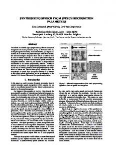
2.8.6 Hidden Events We distinguish between event behaviors which are produced by the reactive system (i.e., messages) and those which are internal to the LSC (i.e., assignments, conditions, and synchronization points). Later, we will construct an automaton which monitors a sequence of visible behaviors and decides whether it satisfies or violates the LSC requirements. It is first necessary to establish a semantics that determines precisely how hidden events are to be carried out based solely on the occurrences of visible events. We present one particular interpretation which will be assumed for the purposes of our construction in Chapter 4. Our interpretation requires hidden events to execute at the instant they become enabled. This means, for example, that if an assignment or condition appears directly below a message on an instance line, it would execute at the same instant as the message. If the assignment or condition is anchored to other instances, it must also be enabled with respect to those instances. Otherwise, it executes upon the occurrence of the first visible event to enable it. Subsequences of consecutive enabled hidden events execute at the same time instant provided each is enabled. If differing linearizations of these hidden event subsequences exist, the LSC chooses one arbitrarily. The chosen linearization could be significant if multiple assignments to the same variable or property exist in the subsequence. To illustrate, consider Fig. 2.3 which depicts two messages and two conditions. We omit the conditional expressions for this example. We first consider the events which occur on instance � only. Since message 1 immediately precedes condition 1 on instance � , it is the case that condition 1 will occur at the same instant as message 1. Condition 2, on the other hand, may only be evaluated once both messages have occurred since it is anchored to another instance. Therefore, condition 2 will be evaluated at the same
C HAPTER 2. LSC R EQUIREMENTS
31
Inst A
Inst C
Inst B
Msg1 Msg2
Condition 1
Condition 2
Figure 2.3: Hidden Event Generation instant as whichever message occurs later in time. Moreover, if message 2 occurs before message 1, then both conditions will be evaluated at the same instant as message 1.
� �
Let � � �/� � be the event trace induced by some LSC run. We impose the followL ing temporal requirements: •
� � �
•
� � �
�
�
�
.�E
�
�
�
F
.�E
F
0
� %
0
EIH�1
� %
EIH�1
�
�
E�H
� E
L �
L
�
F
� � �
��� ���
�
� � �
L L
2.8.7 Chart Satisfaction and Violation
�
�
�/� � ��� � satisfies the A sequence of events � � L � � � prechart of a Universal LSC (denoted � ! � � � ) if � � � , � , � � � � � and ��� - � . � 1 holds. Intuitively, � satisfies L the prechart if it terminates with a satisfying subsequence and causes the bottom-most locations of the prechart to be reached.
�
��
�
�
�
�
�
say that � � �/� � ��� � violates the prechart (denoted � !� � � ) if L � �� � , � We � L � , � � � � , � , ��� - � . � 1 , and �D� > � � � � for � � � ��� . We say � is a minimal � � � ��� . violating sequence if there does not exist such that � � � � , � for ���
��
�
��
An event sequence � LSC (denoted � ! �A ) if
� �
(
�� L
�
�
�
� �
� L
� � �
� � � ��*
�
�
�
!
�
� �
� � �
� �
�
��
�� satisfies main chart of a universal �, � � � ��� the � and � ��� � � holds. �
,
-
. 21
Sequence � � � � � � � violates the main chart, and therefore the requirements, L � � s.t. if there is a subsequence � � � ( � � ��� ��* such that � ��! � � � and either �� � L � � � � � , � or ��� -�� .�� 1 holds.
�
��
�
�
32
2.9. E XAMPLE
2.9 Example To familiarize the unacquainted reader, we present the example of Fig. 2.4. The scenario depicts communication between a user, buffered keypad, and CPU. The prechart states that whenever the user sends ��� �� and then ���� � � � , the interaction appearing in the main chart must follow thereafter. Namely, that Keypad sends the ��� � �� � � � � message to CPU, followed by the CPU sending � � ��� � � to Keypad, followed finally � by the CPU sending ��-�, � � to User.
��
��
��
The example is adorned with horizontal dashed lines to show three points of synchronization, each annotated by the name of the corresponding hidden event. All scenarios begin with the instances synchronized to the top-most location of each instance. � The hidden event which describes the act of synchronization is � � , � . All instances synchronize again at the bottom of the prechart, where event � � � � occurs. In the main chart, all instances synchronize at the bottom-most locations of each instance upon the � occurrence of � � , � . Note that this is a continuation point which signifies a return of control to the prechart.
��
��
User
Keypad
CPU pbegin
PressOn PressKey pend ProcessBuf ClearBuf Notify pbegin
Figure 2.4: Fairness Free Universal LSC We now consider various event sequences and differentiate satisfying behaviors from violating behaviors. For brevity, we omit the identity of the sender and receiver � � instances of a message (e.g., the message � � ��� � � is understood by context to be sent by CPU and received by Keypad). All messages in this example are synchronous, so we use the name of each message to denote the simultaneous sending and receiving of the message. Our discussions consider finite fragments of LSC computations. We begin by considering visible events only. Consider the event sequences � L
�
C HAPTER 2. LSC R EQUIREMENTS
��� � � ��
33
��
��
, � � � � � and � � ��� � � � . Sequence � L satisfies the prechart whereas � violates the prechart. However, . � 1� is not in the language, whereas . � 1� is. This L is because � generates the obligation that the subsequence which follows must satisfy L the main chart (which it doesn’t), whereas the prechart violating behavior of � never creates any obligation.
�
�
Let � � � ���� �� , ��� � � � , ��� � �� � � , � � ��� � � , ��- , � � . This sequence satisfies the requirements since it satisfies the prechart and main chart. Let ��� � ��� �� , ��� � � � , ���� � �� � � , � ��-�, � � . Sequence ��� violates � the� requirements because the prechart is satisfied but � � � �� � � is not followed by � � ��� � � as required by the main chart.
��
��
��
��
��
��
�
��
Until now, we omitted hidden events from the discussion of Fig. 2.4. Let us assume that an object system outputs the visible event sequence � � . From this, the LSC � carries out the sequence � � , � ��� � � � ��� �� ��� ��� � � � ��� � � � � ��� ���� � �� � � ��� � � � ��� � � ��� � ��-�, � � ��� � � � � , � . All computations begin with the hidden event � � , � . Hidden events are executed as soon as they become enabled, and each occurs at the same time instant as the immediately preceding visible event. For example, � � � � oc� curs next in the order and at the same temporal location as ��� � � � . Likewise, � � , � � immediately follows ��-�, � � .
��
��
��
��
��
��
��
��
2.10 Multiple LSC Requirements We now consider LSC requirements consisting of more than one LSC. Traditional methods of scenario composition, such as that seen in MSCs [MSC99], offer the choice of executing multiple scenarios sequentially, alternatively, or concurrently. The choices must be stated up-front by the user using high-level MSCs (hMSCs). In the realm of multiple-LSC requirements, concurrency is dynamic in the sense that a particular set of scenarios may run concurrently, sequentially, alternatively, or any combination thereof, based not on fixed user input but rather on the input behaviors. The dynamic behavioral approach to LSC composition gives rise to the possibility of interesting interactions between several executing scenarios. Multiple LSC requirements share the same set of objects, and therefore the same object properties, but have distinct sets of LSC variables. For this reason, multipleLSC requirements cannot be expressed simply as the product of cuts from each LSC, otherwise duplication of object properties occurs. �
Let � �A ���3')(2� * ����� ��� � ������� .�� 1 represent the set of LSC variable valuations � and the instance-to-location mapping for LSC only. Given an object system and
34
2.10. M ULTIPLE LSC R EQUIREMENTS
LSCs each
L
�/� � ���� , we define multiple LSC requirements by
is an LSC. An m-cut (multi-cut) is the tuple: �
� �
�
� � -
������
�
�
')( +*
L
� � L
�
�
� where
� � � �
�
�
�� � �
In the case of single LSCs, the assertions � , � � � � � and predicate �� � are defined over the valuations in ')( * and ')(2� * for object properties and variables, respectively. For multiple LSCs, there exists only one set of valuations ')( +* but one ')( � * � � valuation for each LSC —each referenced by � . It is understood that when assign� ments or conditions over an LSC variable occur in LSC � , the semantics of � , � � �� � � and � � � are carried out with respect to � . This is assumed to be the case from this point forward.
�� � �
�
We can project an m-cut onto an ordinary single LSC cut with the function � - � � � � Cuts � � NC � -/. ����1 � � to denote the cut � for LSC � in m-cut . We write � . Each single LSC cut has its own successor function ��� - , as we have previously � described. We refer to the particular successor function of LSC � with ��� - � .
� ��
�
��
�
, �,�- .
��
�
A function � Specifically, � � �
��� � - � �� � -
��
�
�
�� � �
�
�
.
�
�
, �,�- .
�
-
E
NC
�
��
�
�
��
- .
����1 1 holds for all � . We write
� - is defined in terms of original cuts. � iff there exists such that for all � �� � - . � ����1 � � ��� -�� . � - . � � 1 � 1 . We say an m-cut � is a successor of whenever � � ��� - . � 1 � � holds for some event .
�
�
�
�
�
The initial m-cut is the m-cut where is initial. 1 to assert that m-cut
�
1
is an infinite sequence of m-cuts
In the spirit of single LSCs, a run of �/� � � , satisfying:
� � � L
•
, �,�- .
�
��
•
� �
� � � �
L
�
�� � ��
� �
(initiality) 1
�
L
� �
�
���
�� � �
-/. �
��1
(consecution)
�
A multiple-LSC computation is a run satisfying G � � � - � ��� . � 1 � > for all � , � where D � � � - � � � � !2- � �� . � - . � � 1 1 �>
. An event trace is the sequence of events induced by a computation. The language of an LSC is the set of all event traces.
�
��
�
C HAPTER 2. LSC R EQUIREMENTS
35
2.11 Self-Spawning LSCs It is possible for a single universal LSC to spawn and execute several instantiations of itself concurrently—a phenomenon we refer to as self-spawning scenarios. This happens, for example, if the LSC is configured to monitor every input for a minimal event— an event which causes the prechart to progress from the top-most locations. Several “copies” of the LSC could therefore exist, each monitoring the input event sequence starting from differing points in the trace.
a b
c a b
Figure 2.5: Self-Spawning LSC Consider the LSC requirements of Fig. 2.5, consisting of one LSC. When the � � messages � � occur, the LSC requires � ��� to occur. By carrying out the required behaviors of the main chart, however, it is possible to satisfy the prechart. This gives rise to a requirement for an infinite cycle of behaviors, namely .�-� �/1 , anytime the prefix -� occurs. We can proceed in one of two directions. The first is to monitor for prechart activation only when the chart is at the initial location. This approach would essentially ignore the prechart whenever the LSC is at a location other than the initial. The second approach is to monitor the prechart at all stages of the execution and permit requirements such as the one in Fig. 2.5. In this work, we choose the former approach in which scenarios cannot self-spawn in this way. That is, we assume one “copy” of each LSC can exist. The main reason for doing this is so we may restrict our attention to a simpler subset of features. Selfspawning scenarios are capable of producing behaviors which could require special handling. For the interested reader, self-spawning scenarios are considered in [PGZ05].
36
2.11. S ELF -S PAWNING LSC S
Chapter 3 Timed LSC Requirements 3.1 Introduction to Time
Many software designs, aside from specifying legal orderings of behaviors, also include timing constraints. Using the previously introduced LSC assignment and condition constructs along with special time variables, LSCs can express timing constraints. We refer to LSCs with such capability as timed LSCs. Timing constraints are generally used to impose upper and lower time bounds on a certain sequence of events, which has the effect of reducing the number of acceptable event traces. Event sequences which are acceptable without timing constraints could become unacceptable if the sequences do not occur within the prescribed time bounds. In this chapter, we consider two particular models of timed LSCs which shall be translated to formal models in later sections. We first consider the simpler case of discrete-time in which time is assumed to be in the domain of natural numbers. Without loss of generality, we further assume that time deltas (i.e., consecutive time units) are separated by a time value of 1. We do not concern ourselves with the specific interpretation of time units; that is, whether the units express minutes, seconds, etc. We follow up the discrete time discussion by considering dense-time LSCs, in which time units are monotonically increasing values expressed over the domain of nonnegative real numbers. Like before, we are not interested in the particular interpretation of time units. However, one important distinction between the two models is that densetime does not assume any fixed time delta. 37
38
3.2. R ELATED W ORK
3.2 Related Work Although several LSC language extensions have been proposed since the seminal LSC paper [DH01], literature on timed LSCs, in particular, has been relatively scant. The first proposal for LSC time constraints to our knowledge was offered in [KW01]. Another scheme, which more closely follows the spirit of the untimed LSC variant, was introduced a year later in [HM02]—our translation most closely follows this approach. The treatment of timed LSCs presented in this chapter is based on the author’s contributions to the work in [PGZ05].
3.3 Single Discrete-Time LSCs We consider LSC requirements which can express time in discrete units. For this purpose, we incorporate a global system clock, ranging over the naturals, into our subset of the LSC language. The system clock is viewed as a special object Clock with a message , � . Execution of , � causes the clock value to increment by 1. The current value of the system clock is depicted on the LSC as Time. All behaviors described by an untimed LSC can be interleaved with occurrences of in a timed LSC. Assignments and conditions similar to those seen in the previous chapter can be used to store Time into a special time-stamp variable (ts-var) and later test time variables with respect to Time. Time-stamp variables range over 0 �,1 where 1 is undefined.
, �
�
Storage of the system clock value into a ts-var is accomplished exclusively using special LSC time assignments of the form “ � � � Time,” where � is a ts-var. Only Time may be stored into a ts-var—constants, ordinary LSC variable or object property r-values are not permitted to be stored in a ts-var. The value of a ts-var may be recalled using an LSC condition restricted to the form “Time = ��� ��� - ” where = � � ��������������� � �:� >
and ��� - is a constant.
�
�
Like LSC variables, ts-vars are undefined at the beginning of each LSC execution. In contrast to LSC variables, however, the range of time-stamp variable values is theoretically unbounded. Consequently, discrete-time LSCs are infinite state systems.
C HAPTER 3. T IMED LSC R EQUIREMENTS
39
3.3.1 Definition We expand the definition of LSCs, as presented in section 2.2, to include ts-vars. Let � ������� ��� ��� � ������ �� I � � �� ��- �/- � �� � , where ����� ��� � � �� �� � � � �� ��- � - � �� are as before and:
�
•
�
�
�
—a set of time-stamp variables, each of which is defined by �� ��� ����� is the name of the variable and ��� 0 �,1 is the value. �
�
�
�
� � � where
The set of ts-vars is defined separately from standard finite discrete LSC variables in order to distinguish between the unbounded ts-vars variables and the bounded LSC � variables. As before, the assertions �� � , � , � , � � � are still applicable to assignments and conditions over the LSC variables and object properties. We will introduce new assertions for dealing with ts-vars shortly.
�� � �
3.3.2 Timed Cuts The set of timed cuts is given by: TCuts
�
Cuts
�
')( �
where Cuts is the set of cuts as seen before and ')(2�
� *
*
is the set of ts-var valuations.
In future sections, we distinguish original cuts from timed cuts by referring to them as untimed or timed cuts, respectively. If is a timed cut, the untimed cut of , written Untime .� 1 , is the projection of Cuts on . We denote by . � 1 the valuation of ts-var � � � � . We use � .� 1 , as before, to project the element of the cut referring to the instance-to-location mapping location. The initial timed cut is given by , ��,�- .��1 � � � � % � � ��2. � 1 � 1 , ��,�-/. Untime .� 1 1 .
3.3.3 Discrete-Time Assertions
�� � �
We characterize the semantics of LSC time assignments using the assertion � , ��� . Given a ts-var assignment - , a timed cut and a time , the assertion states that variable -�� � takes on the value in cut :
�� � � � �
,
�� �
� .�- �
���2.�-�� � 1 � 1
40
3.3. S INGLE D ISCRETE -T IME LSC S
��
We provide a similar assertion,
��
�� .
, for ts-var conditions:
��� . �� � � 1 A �> 1 � 1
� �:� > ���������������
� �
where =
�� �
�� �
� �
� %
� �
�� =
2. ��
�
�
1
��
. Finally,
� � � �1 �� . � 1 �
�
� � .� �
�.� 1
3.3.4 Successor Cuts
� � .� � 1 � � .� 1 , where is understood Similar to section 2.8.4, we use the shortcut to refer to the simultaneous regions in � not appearing in . We say timed cut � over system clock value is a discrete-time successor of if there exists an event � E such � that � � ��� -/.� � 1 . This is the case iff all of the following hold:
�
�
�
�
��� -/. Untime .� 1 � 1 1. Untime .� � 1 � The untimed LSC semantics of section 2.8.4 hold. 2.
�
� -
� �
(V��������.�- 1
%
?
-��
� � �
� * �� � � , � �
� .�-
�
When arriving on a ts-var assignment, store in ts-var 3. 4.
��
� �
1
.
� � - � � ��-�� � � > � � ��������.�- 1 * % , ��,�-/.� � 1 � � � � .� � � � � If ts-var � does not appear in an assignment, then its value is unchanged. � � � � (V������� . �/1 ? % ��� � � � � *� ( �� � � � . � � � 1 � TRUE *
� �
�
� "( (
1 *
Advancing from a condition requires that it evaluate to true. 5.
� �
�
�
�
(V������� . /1
%
?
-
� ��� . /� 1 �A
%
�� �
�
.�
�
� � /1
�
FALSE *
�
, �,�-/.�
�1
Cold
conditions which evaluate to false lead into the initial state. 6.
�1 �
�
, �,�- .�
3
� �
� �� ��.�3 1 � 1
All LSC ts-vars are undefined in the initial state.
3.3.5 Runs and Computations
�� - �
Let G �
cuts � � •
�
L
, �,�- .�
�
�
! -
� ���
.� 1
�>
L
�/� � � , satisfying: 1
(initiality)
�
. A discrete-time LSC run is an infinite sequence of
C HAPTER 3. T IMED LSC R EQUIREMENTS
•
� �
� �
�� �
L
�
�
���
-/.� �
�
�
��1
41
(consecution)
A discrete-time LSC computation is a discrete-time LSC run satisfying: D � � � � . A discrete-time event trace is the sequence of events induced by a computation. The discrete-time language of an LSC is the set of all discrete-time event traces.
��� . � 1 � >
3.4 Single Dense-Time LSCs Within the domain of dense time, values of the ts-vars and system clock both range ���� ). A single dense-time LSC is defined similarly to the over the non-negative reals ( discrete-time case, where: • �
�
—a set of time-stamp variables, each of which is defined by �� ��� ���� 0��,1 is the value. is the name of the variable and ��� �
� � � where
�����
As in the discrete-time case, the set ')( � � * of ts-var valuations is infinite and unbounded. However, these valuations can be mapped into a finite number of clock regions according to [AD94]. The set of timed cuts is the same as in the discrete case, except substituting the new dense-time version of � � : TCuts
�
Cuts
')( �
� *
where Cuts is the set of untimed cuts and ')(2� � * is defined as above. Note that we use the same name � � to refer to the ts-vars for both the dense-time case here and in the previous section for the discrete-time case. This permits us to interchange the two models so as to better express the later results of this work more succinctly. For a timed cut , we again denote by � .� 1 the set of locations belonging to the cut. An instance Clock with message , � is not used, as in the discrete-time case 1 . In our approach, the passage of time is expressed by associating each input event with ���� 1 . Let � � ��an explicit time value. We define a timed event by the 2-tuple .�E � be the infinite set of timed events.
�
�
�� � �
Assertions �� � and � , � are used for characterizing the semantics of LSC assignments and conditions over over LSC variables and object properties. That is, assignments and conditions not involving time constraints. In section 3.3.3, the discrete-time it is possible to use a ��� � message which is parameterized by a dense “real time” value. However, we do not consider parameterized messages in this work. 1 Generally,
42
3.4. S INGLE D ENSE -T IME LSC S
�
�� � � �
analogues �� � � and � dense-time case.
�
,
were presented. We now redefine these assertions for the
�� � �
Assertion � , � � takes three parameters: an LSC assignment -�� � , a timed cut ��� . The latter parameter identifies the time at which � TCuts, and a time value � the assignment itself is carried out.
�� � � � �
,
�� �
� .�- �
���-�� � �
�
�
1
� 1 �
.�-��
�
�
Similarly, �� � � also requires three parameters consisting of a condition ���� . timed cut � TCuts, and time value �
�� .
��
�
�� .
�
�� ��� � � �
1
�
(
� � �A > 1
. ��
%
1
�
� �
�� =
2. ��
Finally, � � � � takes three parameters: two timed cuts � Time 1 we denote the system clock value in timed cut 2 . �
�
� � .�
�� � 1 � �.� 1 � �
.
� 1
�
� . Time 1
.�
�
2.
�
1
�
,
�
�
�� �*
and a ts-var � . By
Time 1 1
3.4.1 Successor Cuts
� � � ������� We define a transition function ��� - � TCuts
� ��NC . Let � � be timed cuts and � � .� � 1 � � .� 1 . We say timed cut � over system clock��value is a � dense-time successor of if there exists an event � E and time � such that � � � � � � . � . � 1 1 . This is the case iff all of the following hold: �
�
�
�
�
�
1. Untime .� � 1 � ��� -/. Untime .� 1 � 1 Assertions over the untimed cuts. 2. 3. 4.
�
-
�
�
�
(V��������.�- 1
?
� �� � � , � � *
� .�-
�
��
1
When arriving on an assignment for ts-var � , the timer value of � is reset to zero.
� � - � � ��-�� � � > � � ��������.�- 1 * % , ��,�-/.� � 1
If ts-var � does not appear in an assignment, then its value is . � � � � (V������� . �/1 ? * ( �� � � � . � � � 1 � TRUE *
� �
�
� "( (
�
�
� � .�
�
�� �
1 *
Advancing beyond a condition in the LSC requires that the condition evaluate to true. 2 This
system clock value can be extracted from a timed cut by reserving a special ts-var and assigning it the system clock valuation.
C HAPTER 3. T IMED LSC R EQUIREMENTS
5.
43
Untime .� � 1 1 ( � 3 � � � �� � .+3 1 � 1)* All LSC ts-vars are undefined in the initial state.
�
, �,�- .
3.4.2 Runs and Computations A dense-time LSC run is a sequence of pairs
�
1.
, �,�- .�
2.
� �
�
3.
� ��� �
4.
� �
(initiality) 1
L
�
��
E
� �� �
���
� �
�
�
�
E
L F
%
��� s.t.
�
��� � � �
�
�
- .� � �.
�
�
�
�
�
�
�
.�
L
� L
�
1 �.�
��1 1
(consecution)
�
(monotonicity)
� 1
�
satisfying:
� � �
(progress)
If � L � � � � � is a dense-time run, then we express the untimed projection of as Untime .� 1 � Untime .� 1 � Untime .� 1 � �/� � . A dense-time LSC computation is L a dense-time LSC run satisfying D � � � -(0 ��� .� 1 , where ��� .��1 is the set of timed cuts appearing infinitely often in and D � � � - � � Untime .��1 ! - � �� . Untime .� 1 1 � >
. A dense-time event trace is the sequence of events induced by a dense-time LSC computation. The dense-time language is the set of all dense-time event traces.
�
�
3.5 Multiple Dense-Time LSCs We now present the formal definitions for dense-time multiple timed LSC requirements. A similar formulation can be applied to the untimed and discrete-time cases, but are not considered here. Multiple timed LSC requirements collectively describe the behaviors of an object system. LSC variables and ts-vars are meta-variables used for the purpose of constraining the behaviors of the objects. Both are unique to each particular LSC and the valuations of both begin in an undefined state at the start of each scenario and become undefined again at the end. In contrast, object property valuations define the state of the object system throughout its entire lifetime. Furthermore, they persist indefinitely, beyond the lifetime of any one scenario. Accordingly, the variables, ts-vars, and the current position of each instance of an LSC are components that are unique to the LSC, whereas object properties are global to all LSCs in the requirements.
44
3.5. M ULTIPLE D ENSE -T IME LSC S
Given an object system and LSCs �/� � ���� , we define multiple timed LSC L requirements by ����� �� � � � � �/���� � where each � is an LSC as defined previously. L
� The state of LSC
�
is given by: � � ���3')( � * 4 ��� � ��� � ��������.+� 1 4 � � ')(2� � * . This represents the set of variable valuations, instance-location mapping, and ts-vars, respectively, for LSC � . The set of ts-vars is assumed to operate in the dense time domain for the purpose of this work, but a discrete time domain could also be adopted. A timed m-cut (multi-cut) is a tuple: �
�
� -
� �
�
������
�
�
')( +*
L
�
�
�
A projection function � - �� � � - #� � �/� � � � � DNC � cut given the unique number of a dense-time LSC. A timed m-cut � m-cut, denoted , ��,�- . 1 iff , ��,�- . � -/. ����1 1 holds for ��� � � � .
��
��
�
�
�
�
yields a timed is an initial timed -
�
�0� E F . For some A visible event of the composed system is defined by EGF � � � � � � E F then � ��� E J . LSC , we assume that if � E�F and � � � � � � � � �� � ��� - � � � - � .�E � 1INC We define � as the transition function of the composed requirements. Let � ��� - � refer to the successor � function of LSC � . We say that �� is a timed m-cut successor of , written � � � ��� -/. ��. � 1 1 , if there exists event and time such that:
�
�
�
�
��
1. 2.
� �
�
� � �
E�F
�
� �
�
�0� E�H
� �
��
� ����1
-/.
� �
��
- .
�
�
� ��� 1 �
�
���
�
�� �
�
-�� .
�
���
� -�� .
�
�
��
��� 1 �� . �
- .
� �
��
�
1 1
��� 1 �� . �
-/.
1 1
Intuitively, visible events cause a synchronous transition to be taken among all LSCs, since each is expected to respond in some way to the occurrence of the event. Each hidden event, on the other hand, represents an internal behavior for just one particular LSC. The case distinction is necessary since LSCs only recognize their own hidden events, otherwise the semantics could be entirely synchronous.
3.5.1 Runs and Computations A dense-time run of ����� �� is a pair . � 1.
�
��
, �,�- .
L
1
(initiality)
� �
-
� � ��� � �� �� � 1
.
L
L
� 1
�� .
��� 1 �/�
� �
satisfying:
C HAPTER 3. T IMED LSC R EQUIREMENTS
�
� �
2. 3.
� ��� �
4.
� �
�
�
� �� �
� � � �
�
��� � � �
� L
E
� %
F
�
�
��� - .�� � ��. � � � � �� � � � �
45
�
�
��1 1
(consecution)
(monotonicity)
(progress)
A dense-time computation� of � ��� � is a dense-time run of ����� �� which satisfies, � for all � , D � � � - � ��� . � 1 � > where G � � � - � � � ! - � �� . � - . ����1 1 � > . An timed event trace of � � � � is the sequence of events induced by a timed computation and the timed language of � ��� � is the set of all timed event traces.
�
�
��
�
3.6 Timed LSC Example We now consider a four-wheeled robotic agent that navigates the perimeter of a roundcornered rectangle drawn in black on a white background. The agent is controlled by a microprocessor with a single light sensor input and an output that controls motor speed for each wheel. Differential wheel power is used to turn the agent left or right. We assume that the agent is initially placed directly over any edge of the rectangle, positioned to travel clockwise as shown in Fig. 3.1.
RCX microcrontroller
light sensor
wheels & steering controller
Figure 3.1: Robot Test Pad To make the LSC more readable, we introduce a special up/down arrow notation on the left side of assignments and conditions to indicate either the preceding (up arrow) or succeeding (down arrow) visible event with which each is associated. The same requirements can be expressed without the use of this notation.
46
3.6. T IMED LSC E XAMPLE
In Fig. 3.3, variable is assigned at the same time instant that message TurnRight � is sent, and the condition over executes at the same time instant that TurnRight is received. User W W SwitchOn H
RCX W W H H
C
Motor
H SetSpeed(3)
H
H
On
H H T := Time
H
Off
H H Time = T + 10
C
C
Figure 3.2: Scenario 1: Switching Robot On The first scenario of this example (Fig. 3.2) describes what should happen when the user switches on the micro controller. In particular, the motor speed is set to 3 and the micro controller switches on the motor. Precisely ten time units after the motor is switched on, the motor is switched off by the micro controller. The second scenario (Fig. 3.3) involves a description of how the agent will navigate the black line. This is carried out by means of a light sensor which is connected to the micro controller. The light sensor can observe two possible conditions: bright or dark. When the agent is over the black line, it senses dark; otherwise, it senses bright. Whenever the agent passes from dark to bright, the sensor sends the micro controller a bright interrupt signal. Conversely, when the agent passes from bright to dark, the sensor triggers a dark interrupt signal. By default, the agent moves straight unless it receives a bright signal, which means that the agent has reached a corner and must start turning right. The second scenario describes this requirement. The LSC of Fig. 3.3 describes the required behavior whenever the sensor sends a bright signal to the micro controller. The specification requires that the agent begin turning no more than 0.2 time units after the sensor sends the signal. Here, we assume that the agent requires zero time to commence a turn and zero time to straighten out the wheels after the turn is complete. If, during the turn, the agent re-intercepts the black line, the light sensor sends a dark signal, which prompts the steering controller to end the turn in no greater than 0.2 time units. Notice that this contrived example does not
C HAPTER 3. T IMED LSC R EQUIREMENTS Light Sensor
RCX
W W
W H H T := Time
Dark
W
TurnRight
H
H T2 := Time H C
Steering Controller
W Bright
W
H
47
C
H
W H Time •
�
���.
1
� �
� �
KML
.
4.3.2 Translation The translation to timed automata follows similarly to the discrete-time case, except that assignments and conditions over ts-vars are not expressed through discrete variables by � means of assertions �� � �� , � , � �� , and � � � � but rather through guards and clock resets. This introduces interesting subtle complexities which are not present in the discrete-time construction.
�� � �
Undefined Time-stamp Variables We have seen in section 3.4.1 that ts-vars take on undefined values ( 1 ) at certain points during execution. The significance is that any undefined ts-var appearing in an LSC condition results in a false evaluation, by definition. As we will see, ts-vars are implemented in our construction by means of timed automata guards. However, timed automata have no notion of undefined clock values and therefore no way to recognize undefined clocks inside a guard, since clocks always map to some non-negative real value. We can express undefined clock values in timed automata by introducing an array of Boolean flags as part of the discrete state space—one flag for each clock. A true flag valuation indicates that a particular clock value is “defined” and that any transition leaving such a state whose guard contains a reference to that clock should be evaluated normally. A false flag valuation, on the other hand, represents an “undefined” value. For
60
4.3. D ENSE -T IME LSC S PECIFICATIONS
each ts-var, it is straightforward to set the corresponding flag to true whenever the ts-var is first assigned in an LSC and false whenever a back-edge to the initial state is taken. Supposing the aforementioned array is present, let us discuss how the information would be used: we first construct the automaton from the LSC under the assumption that all ts-vars are defined, ignoring the flags. After the automaton is built, we remove transitions in the following way. Given a discrete state in which some clock is flagged as undefined (false), we remove all transitions leaving that state in which appears in the guard. The rationale is that the LSC condition—and hence, the corresponding automaton guard—would always evaluate to false, making it impossible to traverse the edge. Below, we will present a translation from dense-time LSCs to a timed automaton. Rather than complicating the construction with the above details, we instead propose to carry out the edge removal as a post-processing step. It is easy to see that the resulting automaton will preserve the semantics of undefined ts-vars, since only guards which test the values of “defined” ts-vars will remain in the final automaton.
Static Evaluation One limitation of timed automata transitions is that clocks may be reset only after the guard has evaluated to true. This presents a complication from the standpoint of our construction, since the successor sequence may dictate an order which the automaton cannot handle—specifically, an assignment followed by a condition over the same tsvar. In this case, we can statically evaluate the condition and modify the transitions to reflect the evaluation. This is possible since ts-var conditional expressions of the form “Time = � � ��� - ,” can be reduced to the expression Time = Time � ��� - .
�
�
msg1
Time �
'
�
� �
� � � �
�
as follows:
�
%
* .�� 1 1
�
, �,�- .
�
.�� 1 1�
• � is the set of transitions �
� �
0
defined below.
� ��
is the set of transitions .�� ��� � � � � � 1 , each with precisely one maximal sucL cessor sequence transition .�� � ����� 1 and each having a maximal successor sequence L / �� � / � � �/����/ � of .�� � 1 such that for all � . � � � � � 1: �
L
� � � � � �� � �� �
1.
,
�
L
.
�
�
.�� �
�
1 �//��1
KML
Semantics for enablement (cf. secs. 2.7.4 and 3.3.4, requirement 1). 2.
�
� -
� �
(V��������.�- 1
?
� �
%
//�
-��
�
� *
(
�� � � � �
,
.
.�� �
Untimed assignments (cf. sec. 2.7.4, requirement 2). 3.
� � �
�
�
.�� .��
� .
� ��� ��1�� ( ( � � 1 � .�� ��1 � � 1 * KML 0
� -
�:-�� � � > � � �
������� .�- 1
KML
1
�
�
.�� ��1 �-��
� ��- �
�
/ � *
Unchanged untimed variable valuations (cf. sec. 2.7.4, requirement 3). 4.
� �
�
�
�
(V������� . /1
?
//�
KML
*
�
( �
�
�
.
.�� �
KML
� 1
� � /1
TRUE *
Untimed (hot and cold) conditions (cf. sec. 2.7.4, requirement 4).
1 *
C HAPTER 4. F ROM R EQUIREMENTS
�
�
�
�
5.
��
L
�
� �
�
6.
�.-��
��
%
�;�
!�-
� � � �� � � �� �
L
�
2.
1
S PECIFICATIONS
���9��� .�- 1
�
!
TO
%
//�
�
%
?
��������. /1
-��
63
�
� � �
?*//�0
where:
� ; � = �
� � �� � � � �
� � � �� � � �
��
2. /1
�
� � � � � �
.��
L
� ��� � � � �� � � � � � � �� � ��� � � ��� � � � � � ��
��
-
-�,
. /1
��
��
��
��
�
� � ��
��� ��
� ��
�� ��������� �� �
� ���
�� ��������� ����
/
��
�� /
1
�
is the set of back-edges. Given the maximal successor sequence transition and one maximal successor sequence / �� � / � � �/����/ � of .�� � 1 , let: L
L
•
L � �/� ���
•
�L�
•
( resp.) be the position of the first false hot (cold resp.) condition in / �� over the LSC variables and object properties, or 0 if none exists.
be the list of all cold ts-var condition positions in / �� .
��
��� � be the list of all hot ts-var condition positions in / �� .
� � �
�
� ��
�
Let .�� ��� � � � � ����� 1 � � if L of the following requirements hold: 1. ( -
�
� ���
�
�9������� . �/1 .�� ��1 1 A �
.
?
%
//�
�>
� ��� . /� 1 �* -
KML
where for some �
�� %
�
.��
�
.
� 1 and all
.�� �
KML
� �
� 1
/1
� .� ( � ��1 , all �
FALSE *
Cold cuts and false untimed cold conditions (cf. sec. 2.7.4, requirements 5 & 6).
� �
2.
�
�
�
(V������� . /1
?
%
/��
KML
�
� ��� . � 1 �
-
�� � � .
.�� �
KML
1
�
� � 1
TRUE *
Hot untimed conditions must be true (cf. sec. 2.7.4, requirement 4).
�
3.
�
� 3
�
� ��� 1/.+3 1 * � 1
.��
Uninitializing untimed variables (cf. sec. 2.7.4, requirement 7). 4.
�
� 3
� � �
.��
����� 1 .�3 1 � 1
Uninitializing ts-vars (cf. sec. 3.3.4, requirement 6).
�
5. 6.
�
�
� �
� �
��
L
�
� � � �� � � �
� �
Let � .�� ��� � � ��� � �� � L
L
!
2. . /
1
L
�
�
1 1�!
��
� �/� �.��
L
#"
�> %
� ��
�/� �
����� � � � � �� ��� 1��
$"
? �
�
s.t. for all ���(� � �
:
64
4.3. D ENSE -T IME LSC S PECIFICATIONS
1. Requirements 2, 3 and 4 above hold. 2. 3. 4.
�
�
/�
���
where �
� � .+� 1
%
�
.
� �
� � � �� � �
. . /
� �� � �
1 1
%
�
#1
�
� � KML
L
� � � �� � �
2. . /
1 1
refers to the condition at position / � in the successor sequence.
We now show that the transitions of the timed automaton faithfully simulate a dense-time LSC computation. In the above construction, we describe the circumstances under which automaton edges are created in three cases: one for forward-edges and two for back-edges. We show that these cases collectively meet the requirements for dense-time LSCs as defined in section 3.4.1. There are five requirements. Requirement 1 states that all untimed requirements from section 2.8.4 hold, and requirements 2-5 are specific to dense-time. The general construction technique is substantially the same as in Theorem 1 for the untimed requirements, with the only difference being a case split on the set of back-edges. It is straightforward to confirm that all untimed requirements hold among the three cases. For each ts-var assignment, rather than storing the fixed value of the system clock at the time of the assignment, we instead reset a clock and refer to the elapsed time inside the subsequent conditions. LSC assignments are carried out by resetting clocks and conditions are implemented as guards. The reader can easily verify that the assertions � � , � �� and �� � �� capture the formal semantics, thereby satisfying requirements 2-4. Requirement 5 states that all ts-vars are undefined in the untimed initial state, and can be met by applying the post-processing procedure described earlier.
�� � �
As in Theorem 1, forward-edges capture successor sequences which terminate in a state from which only visible events are permissible. Unlike Theorem 1, however, there are two sets of back-edges which lead to the untimed initial state. The outcome of a condition over a discrete variable is known at the time of the automaton construction, whereas the outcome of a condition over the ts-vars is not known until the automaton is deciding membership of a timed input word. If a condition over a discrete variable evaluates to false within the successor sequence, there are two cases depending on whether the condition is hot or cold. The first case identifies the first cold condition over a discrete variable in the successor sequence which evaluates to false. An automaton transition leading to the untimed initial state is created and the corresponding guard checks that all hot conditions over ts-vars leading up to this point are satisfied. The second case pertains to the first
C HAPTER 4. F ROM R EQUIREMENTS
TO
S PECIFICATIONS
65
hot condition over a discrete variable in the successor sequence which evaluates to false. If there exists some false cold condition over the ts-vars which occurs before that point in the successor sequence, however, then a transition to the untimed initial state is still possible, thereby avoiding violation. Multiple transitions to the untimed initial state are therefore constructed—one for every cold condition over the ts-vars leading up to that point. The corresponding guards test for the falsehood of each cold condition over the ts-vars. By definition, all timed automata runs satisfy initiality, consecution, monotonicity and progress, and are therefore also dense-time LSC runs. To show that they are also dense-time LSC computations, we observe that the set � of final states above captures the requirement of infinitely many visits to a cold or warm state. �
4.4 Multiple LSC Specifications We turn to the construction of a generalized deterministic timed B¨uchi automaton which accepts the language of multiple timed LSCs � � � � � ��� � . The discrete case is not L treated here because it adds extra detail without offering any new insight. A straightforward automata product construction cannot be immediately applied, for the reasons explained below. First, one may think of the multiple-LSC construction as a synchronous composition of visible events, but an asynchronous composition of successor sequences. That is to say, if multiple LSCs are enabled to carry out the same visible event, then an occurrence of that event will cause all enabled input automata to transition simultaneously. The successor sequence which then follows amounts to an asynchronous interleaving of the hidden events among the input automata. To maintain a deterministic construction, a single interleaving for each .�� � 1 pair must be fixed. The duality between the asynchronous and synchronous semantics requires special handling, which we address in the next section.
�
Next, the object property valuations should be shared between the LSCs in the sense that a change in an object’s property valuation in one scenario should be reflected immediately in all others. A brute-force product construction would wrongly produce independent object valuations. This can be addressed rather easily by redefining the state space so that all object valuations are shared, but everything else—the LSC variables, and ts-vars—are owned by each individual LSC. The third reason is that memory is required for keeping track of whether each LSC
66
4.4. M ULTIPLE LSC S PECIFICATIONS
passes through a final state infinitely often. Rather than add memory variables explicitly, we instead employ a generalized B¨uchi acceptance condition in conjunction with a timed transition system, which yields a generalized timed B¨uchi automaton. This is an automaton whose acceptance component � is instead expressed as a set of accepting sets � � � � � ��� . The requirement is that at least one state in each of the sets occur inL finitely often during a run. Generalized timed B¨uchi automata can be expressed as an ordinary timed B¨uchi automata using known techniques.
4.4.1 Translation We present the main translation result and additional contribution of this work: Theorem 3 Let ����� �� � �� �/� � � �� � be dense-time LSC requirements and L be the language of � � � � . Then there exists a generalized DTBA � � �0' ��� � � such that .�� 1 ?* . ����� �� 1 .
�
� �
.
��� ���
� � � 1 �
�
A single LSC is defined by � � ���3')(2� * ��� � ���3')(2� � * . This ��� � ��������.+� 1 comprises the set of variable valuations, instance-to-location mappings and ts-var valu� � ations for LSC . We denote by � .�� 1 the current valuation of LSC � in state � , and by � as follows: .�� 1 , the current valuation of all LSCs in state � . We construct � •
�
� '
��
��� E
L
F
�
������
�
• � � ')( +*� L We define a partial function � � LSC number, yields a timed cut. • � • �
�
� �
� � �
� .��
L
�
!
����
�/� �
� � �� , ��,�-/. 1
�
� �/�
� �
�
� �
0
�
-
�
� ��� .
�
TCuts which given a state and NC
.�� ���1 1�
where �
• � is the set of transitions �
� �
�
.�� �� 1 1D>
�
.
We start by defining the notion of successor sequences for multiple-LSC requirements. Specifically, we build up to the definition of maximal composed successor sequence transition in a manner similar to the non-composed version. The contents of sets � � and � then follow from the construction of Theorem 2. The notion of successor sequences is similar to the single-LSC case, except that ��� there exist � enablement assertions, distinguished by , � � � ��� � for � � � � � . We
� �
C HAPTER 4. F ROM R EQUIREMENTS
S PECIFICATIONS
TO
67
can express the notion of enablement with respect to a sequence of sim-regions belonging to LSC � using the notation � . In a multiple-LSC setting, successor sequences are an interleaving between the permissible orderings according to each � . The sequence is thus a hybrid of sim-regions among the LSCs. As in the single-LSC case, the chosen interleaving of assignments and conditions over the variables and object properties are respected by the maximal composed successor sequence. There can exist greater than one maximal composed successor sequence. In order to preserve determinism, precisely one must be selected since any larger subset of interleavings may result in a non-deterministic construction. As before, a heuristic function may be employed to choose among the available interleavings. Let � � � � � ��� � be a sequence of numbers ranging over � � � �/� ��� � , where each refers L � to the number of an LSC in the requirements. We write / to refer to a sim-region of LSC � � . Given a state � � � and visible event � EIF , the composed successor sequence ��� �� of .�� � 1 is a sequence of sim-regions / � �A/ � � � � ��/ � satisfying:
�
�
L
�
� /
�
��/ �
��� .
.�� �� 1 1
�
� /
�
��/ �
��� .
.�� �� 1 1
�
�
/
�
��/ �
��� .
.�� �� 1 1
M/
1. 2.
� /
3.
�
/
4.
�
�
� �
� �
�
�
�
� � ���
�
%
�
%
%
�
/
�
/ /
�
�
. /
�
�
. /
� / �
��/ � � �� /
�
�
� /
� /
�
1 � 1
�
/
� �
�
�
EIH �B/
�
The first statement says that each LSC has a sim-region in state � . The second statement says that all sim-regions which are immediate successors of sim-regions in / � are associated with visible event . Each of these events will ultimately cause progress to be made in any LSC in which is enabled. The third requirement states that any simregion other than immediate successors of / will refer to hidden events. This prevents events other than (e.g., other messages) from occurring during the sequence. The fourth statement requires the sequence to satisfy � for all LSCs ��� � � � .
�
�
�
A composed successor sequence / � � / � � � � ��/ � is maximal if for all � and for L ���� � � % � T� W � / � . / 1 � E F . This means that all reachable hidden events all , we have / have been exhausted and only visible events are successors. ���
��
�
Given a composed successor sequence for .�� � 1 we arrive at a state ��� by inducing L � a sequence � �/� � ������� where � � � � � � � � � � ��� - .�� � ��. � . //� 1 � ��1 1 . We call L L .�� � � � � 1 a composed successor sequence transition. As before, a successor sequence transition whose successor sequence is maximal is called a maximal composed successor sequence transition.
�
68
4.5. N ON -D ETERMINISTIC H IDDEN E VENTS
�
Now that we have formally� defined the notion of a maximal successor sequence transition, we construct �� and � according to Theorem 2. For each .�� � 1 , limiting the number of maximal composed successor sequences to one essentially reduces the size of the language by discarding other paths. This reduces the correctness proof of this construction to that given in Theorem 2. �
4.5 Non-Deterministic Hidden Events All of the constructions offered in this chapter assume that assignments and conditions occur at deterministic points in time. Specifically, at the same time instant that they become enabled, which is also the same time instant at which the preceding visible event occurs. The overall semantics are generally the same, with the differences resting mainly in the minor details. We’ve also noted that smart play-out differs from our approach in that it uses a less restrictive semantics for determining the time at which to execute assignments and conditions. It is reasonable to ask why we have not chosen similar semantics for our constructions in this chapter. Intuitively, such a construction would require a means to execute hidden events temporally between visible events, rather than at the same time instant. A so-called silent transition (otherwise known as -transition) variant of timed automata would seem necessary so that transitions could fire without an accompanying event. As one might expect, such an addition introduces non-determinism. It turns out that there are other side-effects in the case of dense-time. The original timed automata work of [AD94] does not include any notion of silent transitions. The issue of adding silent transitions is considered in [BGP96], and concludes that doing so can add expressiveness to the language. That is, it can result in an automaton whose language cannot be expressed by any timed automaton without silent transitions. Later, in [DGP97], it is further shown that the introduction of silent transitions does not add expressiveness if no clocks are reset on the transition. Moreover, silent transitions with resets may also occur, but may not appear on any directed cycle. It seems problematic to implement the semantics of non-deterministic LSC assignments in timed automata. Specifically, since a dense-time assignment is implemented as a clock reset, a silent transition with a clock reset is required. All paths in an LSC automata—according to our subset of features—lie on a directed cycle, thereby making the above results unusable for relating the expressiveness of the automaton with silent
C HAPTER 4. F ROM R EQUIREMENTS
TO
S PECIFICATIONS
69
transitions to one without. We believe it may be still possible to prove LSC automata, in particular, exempt from the problems above despite the presence of cycles. Nevertheless, additional problems exist. Recall that a successor sequence can, in the general case, contain an arbitrary interleaving of assignments and conditions. Although, according to the nondeterministic interpretation, it is unnecessary to group together the successor sequence temporally, a construction method for dealing with arbitrary sequences is still necessary. However, it is unknown to us at present whether an algorithm for removing silent transitions from arbitrary successor sequences is decidable.
70
4.5. N ON -D ETERMINISTIC H IDDEN E VENTS
Chapter 5 Automata-Based Synthesis Going directly from requirements to a correct implementation has long been a “holy grail” for system and software development. According to this vision, instead of implementing a system and then working hard to apply testing and verification methods to prove system correctness, a system is rather built correctly by construction. Synthesis is particularly challenging for reactive systems, in which the synthesized system must satisfy the requirements for any possible behavior of an external environment [ALW89, Dil89, PR89a]. The problem of constructing reactive systems directly from formal requirements dates back to Church’s problem in 1963. Various solutions to the problem have since been proposed; for example, see [BL69, Rab72]. Due to the widespread interest in Linear Temporal Logic (LTL), synthesis using LTL formulas as requirements has also been considered [PR89a]. In the general case, time complexity for most of these solutions is intractable due to the theoretical double exponential lower bound [PR89a]. Despite this, recent work focuses on various subsets of LTL [AMPS98, AT04] whose time complexity is suitable for building tools of practical use. It turns out that one particular subset is sufficient for the purposes of synthesizing from many interesting LSC requirements. The subset in question is the recurrence property seen previously—“infinitely often, the LSC must be in its prechart.” Moreover, the synthesis problem for this subset has been shown [PPS06] to be solvable in polynomial-time. In this chapter, we introduce an automata-based algorithm for solving the synthesis problem for LSCs, specifically. We will see that the worst case time complexity of the algorithm is linear in the product of states, edges and inputs.
71
72
5.1. R ELATED W ORK
5.1 Related Work There have been considerable efforts to synthesize executable systems from scenariobased requirements [KM94, KMST96, LMR98, KGSB99, WS00, WSK03, UKM04, LDD06]. In many of these papers, the requirements are given using a variant of classical message sequence charts while the synthesized system is state-based. Although there are many common aspects to our work and these papers, the main distinguishing feature is that we consider synthesis from LSCs, which we have already seen is more expressive than most of the classical MSC variants. Synthesis from LSCs was first studied in [HK02], and is tackled there by defining consistency, showing than entire LSC requirements are consistent iff they are satisfiable by a state-based object system. A satisfying system is then synthesized. This line of work was continued in [HKP05] which includes an implementation of a sound but not complete algorithm for Statechart synthesis. A game theoretic approach to synthesis from LSCs involving a reduction to parity games is described in [BS03a, BHS05]. Synthesis from LSCs using a reduction to CSP is described in [SD05]. All the above papers were either theoretical and did not include an implementation, or the synthesis approach was sound but not complete, or the initial experimental results were not encouraging. An alternative strategy for synthesis from LSCs uses a translation from LSCs to temporal logic [KHP 05] or automata [KW01] and then applies existing synthesis algorithms, e.g., [PR88, Var95, JB06].
5.2 Smart Play-Out The Play-Engine [HM03] is a software package which enables users to create and execute LSC requirements based on the so-called play-in/play-out approach [HM03]. Playin provides an intuitive method to capture requirements by manipulating the graphical interface of the system, while play-out executes the scenarios in a way that gives a feeling of running an implementation of the system. An improvement called smart play-out, is introduced in [HKMP02]. Smart playout uses verification methods—in particular, model-checking—to run LSC requirements and avoid certain LSC violations that may occur for the original version of play-out. One of the shortcomings of smart play-out is that the executable traces it generates are not guaranteed to avoid all violations of the LSC requirements. The following results overcome the limitations of smart play-out by guaranteeing non-violating behavior for all scenario executions. We consider requirements in which
C HAPTER 5. AUTOMATA -BASED S YNTHESIS
73
certain objects participating in the scenario represent the system to be constructed and the rest represent an external environment. We assume open systems which assume no environment cooperation in satisfying the requirements. Unlike [KHP 05], we intentionally shift much of the LSC logic from a temporal logic formula to the finite discrete system so as to potentially reduce synthesis time complexity and focus our attention on a simpler generalized B¨uchi temporal logic formula that has a better chance of success in practical settings. We view the synthesis problem over LSC requirements as a two-player game between the system and the environment. The system refers to the collection of software, hardware, or conceptual objects which are within the immediate control of the reactive system. Conversely, the environment refers to the collection of objects which are external to the program, and whose behaviors are beyond the control of the system. The system attempts to win the game by taking whatever legal actions necessary to satisfy the requirements. Legal actions refer to a subset of the behaviors permitted by the requirements. The environment attempts to foil the system by preventing it from satisfying the requirements. Thus, the environment’s goal is the negation of the system’s. The environment has the upper hand because the system usually needs to meet numerous behavioral criteria in order to win, whereas the environment need only find one way to prevent the system from winning.
5.2.1 An Example To illustrate why synthesizing LSC requirements is important, we present Fig. 5.1, consisting of two universal LSCs. Instance U SER belongs to the environment, while T REE and N OISE are system instances. Accordingly, the behaviors of T REE and N OISE are within the control of the system we intend to construct, whereas the behaviors of the U SER are assumed to be external. According to LSC1, whenever U SER sends the wake message, the system must respond with a non-deterministic ordering of message fall and make in order to satisfy the main chart. Therefore, the traces wake , fall , make or wake , make , fall are both acceptable for satisfying LSC1. On the other hand, LSC2 is an anti-scenario which states that the sequence make , fall , sleep cannot ever occur. The synchronizing conditions remove the otherwise non-deterministic ordering of make , fall , sleep to ensure that only traces with this precise ordering will satisfy the prechart.
74
5.3. OVERVIEW LSC 2
User
Tree
Noise
LSC 1
User
make Tree
Noise
SYNC
wake
fall SYNC fall
make
sleep
FALSE
Figure 5.1: LSC Requirements for Smart Play-Out We now consider how smart play-out might respond to an input message wake . After formulating a model-checking problem that attempts to verify the non-existence of a satisfying LSC1 trace, the resulting counter-example yields one of the two possible event sequences above. Supposing that smart play-out executes the sequence: make , fall , LSC1 would be satisfied, but the prechart of LSC2 would advance such that the next enabled message is sleep . The environment could then execute sleep and violate the requirements. This illustrates the inability of smart play-out to look ahead into the future by more than one super-step. Using synthesis, it is possible for the system to decisively choose an alternative sequence that would not allow the environment to violate the requirements. In response to the message wake , the synthesis algorithm would have removed the transitions that permit the sequence make , fall to occur, leaving fall , make as the only existing path.
5.3 Overview The synthesis problem is broken down into two parts. The first part is the realizability question, which asks whether or not there exists some way for the environment to win the game. If the answer is in the negative, then the system is said to be realizable. The second part of the problem is to formulate a winning strategy for the system, provided the system is realizable. The winning strategy is like a road map which guides the system in producing behaviors that will always satisfy the requirements. Let be multiple untimed LSC requirements over an object system . We first translate into an automaton using the discrete-time multiple LSC construction of sec-
C HAPTER 5. AUTOMATA -BASED S YNTHESIS
75
tion 4.2.2. Note that the untimed construction is just a specialized case of discrete-time, whereby the set � � of ts-vars is empty. Recall that we solve the synthesis problem by formulating a two-player game between the system and environment. For the purposes of synthesis, the automaton must be converted into what we call a game structure, suitable for the purposes of game play. The two models are substantially the same, except that the transitions of the game structure are partitioned into two disjoint sets, necessary for identifying the transitions of each player.
5.4 Game Structures A game structure is defined by •
is a set of states.
• '
is the set of events.
• �
is the set of initial states.
•
��� ����� ?
•
�4?
#'
� � ��' ��� ����� ����� � � � , where:
are the set of environment and system transitions.
is the accepting set.
Notice that there exist two transition sets, ��� and ��� , whose purpose is to identify the legal moves for each player at any given state. The intuition is similar to a board game such as Chess: just as Chess players are only permitted to move their own pieces, we similarly require that each player can only move between states using their own transitions. The process of identifying which transitions belong to which player is carried out as follows. Given an object system , recall that each object � � is owned by either the system or environment. That is, �$� ��� � � � � � � �M . We partition the objects of into two disjoint sets according to their ownership. Using this information, we assign ownership to LSC messages. Specifically, messages sent by the environment are classified as environment messages, whereas those sent by the system are system messages. Since messages are defined, in part, by the LSC locations to which they are associated, we can map these locations to visible events by means of function �� ��- .
� �
�
To summarize the above: by partitioning the set of objects, we arrive at a partitioning of the set of visible events. Let '�� be the set of environment events, and '�� be the set of system events induced by this object partitioning. If we let ' � '��Z0#' � , we
76
5.5. G AME RULES
�
can identify every transition system if ��' � .
�
�1
� ��/
.�/
�
as belonging to the environment if
�
'��
, or the
Ownership of hidden events, on the other hand, depends on the owner of the preceding visible event, as discussed in section 2.8.6. Therefore, hidden event ownership is dynamic, whereas visible event ownership is static. Fortunately, we need not concern ourselves with hidden events since the semantics are handled implicitly by the automaton construction.
5.5 Game Rules is a sequence of states / ��/ �
A play of game structure 1. Initiality: / L
�
2. Consecution: �
�
3. Reactivity:
. / �
�
�
�
�
�
� �//�
�
L
. / �
L
1
�
� ��/ �
���
�
L
1
�
��� 0
�/� �
, satisfying:
���
, for infinitely many � .
�
The behaviors of the game follow the � -regular expression .�' � �' � � 1 , where the environment executes an event in '�� and the system responds with a super-step 'I� � consisting of zero or more events. Since the system may choose empty super-steps, event traces could consist of events entirely in '�� . However, the system is not permitted to block environment input by prolonging its super-step to infinitely many events—hence, the third requirement above which states that environment events occur infinitely often 1 . We also require super-steps to be atomic in the sense that the environment is not permitted to interrupt the super-step by injecting a ' � event. This is justified because in real-life systems, environment inputs are often buffered—for example, in a FIFO queue—while the system processes events at the front of the queue. The synchrony hypothesis allows us to ignore issues of timing and queue boundedness which are beyond the scope of the current work. We also require that environment messages only appear in precharts 2 . To see why this is necessary, we first note that the system is responsible for choosing super-steps 1 One
may model “no environment input” using a self-loop labeled by a reserved no-op sym-
bol. 2 This
assumption is necessary for the current result, but not necessary in general. We later discuss a winning condition which does not require this assumption.
C HAPTER 5. AUTOMATA -BASED S YNTHESIS
77
that satisfy the requirements. Allowing environment messages to appear in the main chart would have the effect of creating future obligations for the environment. However, in a real-life setting, the environment could trivially violate the safety properties by producing the wrong behavior or not producing any behavior at all, thereby leading to unrealizable requirements. To remedy the above problem, one might impose artificial assumptions of the environment which state that the environment will cooperate by producing the expected behavior whenever a main chart requires the behavior to occur. However, since the purpose of this work is to underline the hostile and unpredictable nature of the environment, we felt it counterintuitive to take this approach.
5.6 The Synthesis Problem Let be a game structure with accepting set � . We say that a game structure satisfies � , written !� � iff for all paths of , some state in � occurs infinitely often. Formally, the synthesis problem is defined in two parts: 1. Realizability: Given a game structure � ��� such that � !� � ? with � � ��� ? 2. If so, construct
with accepting set � , does there exist
�
�.
In the sections to follow, we present a decision procedure for realizability checking. Later, we show how to arrive at the winning strategy, provided the specification is realizable. Construction of the strategy amounts to deciding which transitions, if any, to remove from .
5.6.1 Definitions
� ���
�
We say that a state / � is stable, denoted - � � . /�1 iff � � �$( � � . / � � ��/ � 1 � ��� * . That is, iff every environment input is enabled from / .
�
'
�
M/ � �
Stable states are precisely those in which all LSCs are located somewhere within a prechart. This follows from our above assumption that environment messages cannot appear in the main chart—indeed, if any of the LSCs were in a main chart, then no environment inputs would be enabled. Hence, all LSCs are in their prechart.
78
/
���
5.6. T HE S YNTHESIS P ROBLEM
�
�
A super-step path by is a path between two stable states / ��/ (denoted / L ), such that / C where . / � ��/ 1 � ��� and for all ��� � ��� , . //� � ��//� �C / L L . If we aren’t interested in the identity of event , we simply write / / .
�����
�
�� �
A stable state is controllable if for all � by . State is said to be forward controllable to /
/
�� /
� � /�
/
is controllable. Set � ? is stable and forward controllable to � .
/
�
�
�
. /
%
/
�
�/
�1
� L L
� 1
�
L
���
there exists a super-step path � ? iff / is controllable and for all is a forward controllable set if each
5.6.2 Main Result Theorem 4 (Realizability) Let be a game structure where winning condition � � ��� � . /�1� . Then there exists � with � � ���I? � ��� such that � !� � iff there exists �,/ ! - � � a forward controllable set � ? in s.t. / � � .
"�
Proof:
�
Since there are finitely many states in � , all paths leaving / must therefore lead to a cycle of stable states. Let � be the set of states of � and begin with the edges of . Let be the set of states belonging to any super-step leading out of any state in � . Remove from � any edge which leads to a state outside of . The remaining edges are guaranteed to lead to some other / � � � , since � is a forward controllable � set. Clearly, � ? . Moreover, since all paths from / lead to a cycle of stable states, we have � ! � � . �
�
�
�
Let � be the set of stable states in � reachable from and including / . We show that this set is forward controllable: Since � ! � � , all paths leading out of states in � lead to a cycle of stable states. Let be the set of stable states appearing in any cycle. Since every state in is in a cycle, each stable state in the cycle is controllable, since each leads to another stable state. Since every state in is controllable, must be forward controllable. Now consider the set of states � ? � which aren’t in . Since � !� � , these states all lead to . Hence, � � �(0; is forward controllable. �
5.6.3 Algorithm We present a two-part algorithm for deciding realizability, written in pseudo-BASIC. The main idea is to determine the existence of a forward-controllable subset of , which by Theorem 4, is equivalent to deciding realizability. The first part places tokens on
C HAPTER 5. AUTOMATA -BASED S YNTHESIS
79
states and propagates them across the game structure to determine all-pairs reachability among the stable states. In the second part, we identify uncontrollable states (stable states having no reachable successor), remove these states, determine whether this removal affects the controllability of other stable states, and repeat until we converge on the (possibly empty) set of forward controllable states.
�
In the algorithms below, ��� ����� denote the transition relations for the environment and system, respectively. Each contain transitions of the form . / � � ��//��1 where / is the origin state, / � is the destination state and � is the event label, indexed by � . We let ��� � .�/�1 and ����- ��� � � � ��� � . /�1 be assertions stating that state / is stable or controllable, - � repsectively.
�
�
Algorithm Part 1, presented in listing 5.1, contains two main loops. Within the first loop, tokens are placed on all states which are adjacent to a stable state. We assume a mapping of ' � to a finite subset of the naturals, such that every outgoing transition is assigned a number according to the outgoing transition’s event. Each token (2/ � ��* contains information identifying both the identity of the stable state / and the number of the transition � from / which originated the token.
Listing 5.1: Algorithm Part 1: State Marking Let Let
�
:= � ����� � � �� ����
����������� ��� �! "�#�%$ � For each ��&'����� � � �� � and a l l "�)(%* � (%� � � i n + � P l a c e t o k e n ,-��