Earth and Planetary Science Letters 311 (2011) 351–363
Contents lists available at SciVerse ScienceDirect
Earth and Planetary Science Letters journal homepage: www.elsevier.com/locate/epsl
Synthetic images of dynamically predicted plumes and comparison with a global tomographic model Elinor Styles a, Saskia Goes a,⁎, Peter E. van Keken b, Jeroen Ritsema b, Hannah Smith b a b
Department of Earth Science and Engineering, Imperial College London, London, SW7 2AZ, UK Department of Earth and Environmental Sciences, University of Michigan, Ann Arbor, MI 48109-1005, USA
a r t i c l e
i n f o
Article history: Received 28 February 2011 Received in revised form 3 August 2011 Accepted 8 September 2011 Available online 21 October 2011 Editor: Y. Ricard Keywords: mantle plume seismic tomography plume dynamics shear velocity
a b s t r a c t Seismic detection of a mantle plume may resolve the debate about the origin of hotspots and the role of plumes in mantle convection. In this paper, we test the hypothesis that whole-mantle plumes exist below major hotspots, by quantitatively comparing physically plausible plume models with seismic images following three steps. We (1) simulate a set of representative thermal plumes by solving the governing equations for Earth-like parameters in an axisymmetric spherical shell, (2) convert the thermal structure into shear-velocity anomalies using self-consistent thermo-dynamic relationships, and (3) project the theoretical plumes as seismic images using the S40RTS tomographic filter to account for finite seismic resolution. Simulated plumes with excess potential temperatures of 375 K map into negative shear-wave anomalies of up to 4–8% between 300 and 660 km depth, and 2.0–3.5% in the mid-lower mantle. Given the heterogeneous resolution of S40RTS, plumes of this strength are not easily detectable if tails are narrower than 150–250 km in the upper-mantle or 400–700 km in the lower mantle. In S40RTS, more than half of the forty hotspots we studied overlie low-velocity anomalies that extend through most of the lower mantle. These anomalies exceed 0.6% in the lower mantle, compatible with thermal plume strengths. They have widths mostly with the range 800–1200 km, which is at the high end of plausible thermal plume structures, and at the low end to be resolved in S40RTS. In the upper mantle, the shear velocity is low beneath more than ninety percent of the hotspots. For about ten, including Iceland, the East African hotspots, Hawaii, and the Samoa/Tahiti and Cobb/Bowie pairs, S40RTS low-velocity anomalies extending through the transition zone imply 200–300 K excess temperatures over a ~1000 km wide region. This is substantially broader than expected for thermal plume tails. Such anomalies may be compatible with deep-seated plumes, but only if plume flux is strongly variable due to, for example, interaction with phase transitions and/or chemical entrainment. © 2011 Elsevier B.V. All rights reserved.
1. Introduction Hotspots such as Hawaii and Iceland are characterized by excess volcanism and topography that are not explained by the plate tectonic paradigm, and their origins remain debated (see review by Ito and Van Keken (2007)). Morgan (1971) first attributed hotspots to narrow mantle plumes that rise vertically from the core–mantle boundary (CMB). In the past forty years, numerical and laboratory simulations have illustrated that plumes can vary strongly in morphology and flux, especially if chemical buoyancy effects, non-linear rheology or large scale mantle flow are taken into account (e.g., Davaille et al., 2005; Van Keken, 1997). Seismic methods constitute our highest resolution mantle probe. Hence, a critical test of the plume hypothesis relies on the seismic
⁎ Corresponding author. Tel.: + 44 20 759 46434; fax: + 44 20 759 47444. E-mail address:
[email protected] (S. Goes). 0012-821X/$ – see front matter © 2011 Elsevier B.V. All rights reserved. doi:10.1016/j.epsl.2011.09.012
imaging of the mantle beneath hotspots. Several seismic models do image low-velocity anomalies from the surface to deep in the mantle below a number of major hotspots (Bijwaard et al., 1998; Boschi et al., 2007; Davaille et al., 2005; Li et al., 2008; Montelli et al., 2006; Obrebski et al., 2010; Rhodes and Davies, 2001; Ritsema and Allen, 2003; Tian et al., 2009; Wolfe et al., 2009; Zhao, 2004). For example, a number of P and S wavespeed models exhibit continuous low-velocity anomalies below Hawaii, Afar and Samoa (Fig. 1a), but the same models suggest that the low-velocity anomaly beneath Iceland is confined to the upper mantle (Fig. 1b). However, the models reveal different morphologies and different strengths of the seismic anomalies. It is likely that differences in the used data sets and applied inversion techniques contribute to the image differences. It is therefore critical that the interpretation of the seismic images is accompanied by a quantitative analysis of the image resolution. In this paper, we compare low shear-velocity anomalies below major hotspots in model S40RTS (Ritsema et al., 2011) with the anomalies predicted from a mineral-physics-based conversion of numerically simulated thermal plumes. Previous studies have determined
352
E. Styles et al. / Earth and Planetary Science Letters 311 (2011) 351–363
(a)
S-wave models Montelli et al. (2006)
Ritsema et al. (2010)
−16
40˚
P-wave models Li et al. (2005)
−16
0˚
−16
40˚
0˚
20˚
Bijwaard et al. (1998)
0˚
−16
0˚
40˚ 20˚
0˚
−0 .6
20˚
−0.4
20˚
0˚
0˚
.64 −0
.6 −0 −0.4
429km
40˚
0˚
−0.2
440km
6 −0.
− .4 0.8
−0.2 −0.6
−0.2
2
−0.
627.5km
−0
1017km
1830km
−0.4 −0 .2
−0 .4
−0
610km
.6
1040km
−0
1900km
.6 .4
−0
2236km
2300km
(b)
−40
˚
80˚
−40
˚
0˚
0˚
80˚
60˚
−40
˚
−40
˚
0˚
0˚
80˚ 60˚
80˚
60˚
60˚
.6
−1
−0
429km
.4
.4
.4
−0
610km
440km
−0.2
−0
−0
627.5km
.2
−0 −0.8 −0 .2
1017km
1830km
1040km
−0.2
1900km
2236km 2300km
% −1.2 −0.6 0.0
0.6
1.2
dVS
% −0.6 −0.3 0.0
0.3
0.6
dVP
Fig. 1. Illustration of imaged seismic structure below Hawaii (a) and Iceland (b) with four independent seismic tomography models, using different data sets, different theories and different inversion procedures. Slices are at depths of 429, 610, 1017, 1830 and 2236 km for the Montelli et al. (2006), Ritsema et al. (2011), and Li et al. (2008) models, and at 440, 627.5, 1040, 900, 2300 km depth for the Bijwaard et al. (1998) model. Slow S-wave velocity anomalies are contoured every − 0.2%, P-wave velocity anomalies every − 0.1%. On the S40RTS (Ritsema et al., 2011) slices, the location of the maximum slow shear-wave anomaly within a 1000 km radius of the surface hotspot location is marked by yellow stars. Below Hawaii, all models display strong, wide upper mantle anomalies, and relatively continuous low-velocities throughout the lower mantle, except for in the Bijwaard et al. (1998) model which has little resolution in the lower mantle below this part of the world. Below Iceland, all models image upper mantle anomalies similar in width but stronger in amplitude than those below Hawaii, and they also agree on a relatively weak and patchy structure in Iceland's lower mantle.
possible seismic signatures of mantle up- and downwellings (e.g., Bina, 1998; Goes et al., 2004; Kreutzmann et al., 2004; Ricard et al., 2005), and others performed qualitative comparisons between dynamic and seismic plume structures (e.g., Davaille et al., 2005; Kumagai et al., 2008). Here we make dynamic and seismic model comparisons more quantitative by accounting for tomographic resolution. Our analysis
consists of three steps: (1) we use a set of dynamical models of mantle plumes with different morphologies; (2) we convert the dynamical structures into seismic velocity using a self-consistent thermo-dynamic approach; and subsequently (3) we apply the S40RTS resolution filter to compare the predicted seismic expression of plume models with the tomographic model structure below hotspots.
E. Styles et al. / Earth and Planetary Science Letters 311 (2011) 351–363
2. Dynamical mantle plume models 2.1. Plume characteristics from previous models How a structure is viewed seismically depends on the anomaly amplitude, the size of the anomaly (relative to wavelength of the seismic waves used) and its location relative to the distribution of seismic sources and receivers. Excess temperature and plume width as a function of depth are thus the key parameters controlling the seismic plume expressions. Plume tilting may also affect how a structure is imaged, but it depends on uncertain and model-dependent global-scale flow. Laboratory and numerical plume experiments have been conducted under a large range of assumptions about the mantle rheology, the role of compositional buoyancy, effects of phase transitions, or the presence of large-scale 3D flow. Within the rich diversity of plume morphologies and dynamics, we can make a number of general observations. Most plumes are characterized by an initial rise from a thermal boundary layer, often with a large head leading a thinner tail (e.g., review by Ribe et al., 2006). In models with a lower-viscosity upper mantle, the plume head and tail thin significantly. Once the plume head has spread horizontally below the top of the model (which would represent the base of the lithosphere) the plume tail may reach a mostly steady-state structure. These (nearly) steadystate plumes share several characteristics. First, their diameters generally increase with depth. Plumes may broaden rapidly over narrow depth intervals (e.g., across the 660-km phase transition), or smoothly with depth where viscosity increases gradually with depth. Plume tail diameters range from hundreds of kilometers in the lower mantle to few tens to few hundred kilometers in the upper mantle (e.g., Goes et al., 2004; King and Redmond, 2007; Van Keken and Gable, 1995; Van Keken et al., 1993). Second, the temperature contrast between the plumes and surrounding mantle increases with depth. Petrological, topography, and seismic constraints indicate excess temperatures below hotspots (relative to mantle average) of 100–300 K (Herzberg et al., 2007; Ito and Van Keken, 2007). The excess temperature at the base of the mantle can be up to a factor of three higher depending on the relative importance of adiabatic compression, internal heating and conductive cooling during plume ascent (e.g., Albers and Christensen, 1996; Bunge, 2005; Loper and Stacey, 1983; Zhong, 2006). Third, strong shearing by moving plates can significantly alter mantle flow and bend plume conduits (Farnetani and Hofmann, 2010; Steinberger and O'Connell, 1998). The morphology of the plume head and tail can be time dependent if there is strong feedback between thermal and chemical buoyancy (Kumagai et al., 2008; Lin and Van Keken, 2005; Ribe et al., 2006; Samuel and Bercovici, 2006), non-linear rheology (Van Keken, 1997) or effects of the phase changes (Farnetani and Samuel, 2005). In these cases, pulses of hotter material traveling up the conduit result in irregular changes in width and temperature with depth, and shearing by mantle flow results in complex structures (Farnetani and Samuel, 2005). 2.2. Model plumes used for sensitivity tests We analyzed the seismic signature of a wide range of regional (i.e., without outside mantle or plate flow effects) models of plumes, with different excess temperatures, with various formulations of mantle viscosity and expansivity, different phase transition parameters, as well as models with and without a compositional contribution to plume dynamics (Lin and Van Keken, 2006b). To illustrate the effects of seismic sensitivity and resolution, we chose four numerical simulations of plumes with different morphologies (Fig. 2). All four models are dynamically purely thermal with the same excess temperatures. We assess the influence of composition on seismic
353
plume expressions by assigning an anomalous composition to the core of one of the plumes. Three of these four models represent nearly steady-state plumes with a variable influence of phase transitions. Model P0s has no phase transition effects. Models P2s and P4s include phase boundaries near 410 and 670 km depth. Both models implement an exothermic phase boundary with a 3 MPa/K Clapeyron slope for the 410-km boundary. For the 670-km boundary we use an endothermic phase boundary with a Clapeyron slope of either − 2 MPa/K (P2s) or −4 MPa/K (P4s). A fourth case, denoted P0h, corresponds to an earlier phase in the evolution of Model P0, where the head is transiting the upper mantle. The model set-up is based on Lin and Van Keken (2006a). It employs an axisymmetric spherical shell geometry, with an average mesh resolution of 8 km and refinement to 2 km in the regions near the corner of the plume axis and the core. The simulated plumes ascend from a thermal boundary layer at the core–mantle boundary. The governing equations are the conservation of mass, momentum and energy under the anelastic liquid approximation (King et al., 2010). This accurately accounts for the effects of compressibility of the mantle. These models are similar in design to those by Leng and Zhong (2010). In this series of models we assume a modest thermal boundary layer excess temperature of 600 K (e.g., Farnetani, 1997; Ribe et al., 2006) resulting in near-surface excess temperature of 375 K, near the high end of plume-temperature estimates from petrology (Herzberg et al., 2007). We use an Adams–Williamson equation of state, where the adiabatic dimensional reference temperature is given by Ta = Ts exp (Di∙ z), with dissipation number Di = αgH/cp = 0.68 (α is thermal expansivity at the surface, g gravitational acceleration, H the depth of the mantle and cp specific heat), and Ts the potential temperature (set to 1600 K). Depth-dependent expansivity decreases from top to bottom by a factor of 3, while diffusivity increases with depth by a factor of 4 following the equations in Van Keken (2001). The viscosity is given by η(T,z)=A(z)exp(−b*(T−Ta)). A(z) introduces a step-wise 30-fold decrease in viscosity from lower to upper mantle. The temperature factor b=ln(102) results in a factor of 100 lower viscosity inside the plume. Ta is the adiabatic temperature Ta =Ts ·exp(Di z/γ) where the Grueneisen parameter γ=1. The Rayleigh number (based on lower-mantle background viscosity and surface values of diffusivity and expansivity) is 1.52∙106. The initial condition includes a 100-km thermal boundary layer that is slightly perturbed at the plume axis. Under these conditions, the plume rises through the lower mantle in approximately 30 Myr. Once it reaches the transition zone, it penetrates rapidly into the upper mantle and thins by a factor of 2–3 (Fig. 2a). While rising, the head forms a mushroom-type structure with a hot core and a warm cap, which gets pinched as it transits from the lower into upper mantle (Fig. 2b). At the surface, the plume spreads and forms a few thousand kilometers wide hot region in the upper 200–300 km of the mantle. Even in Model P0, where the effects of phase transitions are ignored, the plume flow through the 670-km boundary is initially somewhat episodic due to the viscosity contrast, but it reaches a nearly steady state after approximately 80 Myr (Model P0s, Fig. 2a). In Model P2s, the plume also penetrates into the upper mantle but it has stronger time-dependent behavior. A portion of the original plume head remains in the uppermost lower mantle as a ring around the plume conduit (Fig. 2c). If the ‘660’ Clapeyron slope is more negative (Model P4s), the phase boundary is sufficiently strong to inhibit plume penetration in the upper mantle (Fig. 2d). This case represents a failed plume that may exist in the lower mantle without a corresponding surface expression. The heat transport characteristics of our model plumes fall within the range of plume buoyancy flux estimates from Sleep (1990), which are 1.7 Mg/s for Iceland and 8.3 Mg/s for Hawaii. The model buoyancy flux of the plume models is derived by integrating ραw(T − Ta), where w is the upward velocity. In the models with time-dependent
E. Styles et al. / Earth and Planetary Science Letters 311 (2011) 351–363
−800
0
−2−1
50
−1
−1 −1 −2 −1
150
(b)
2400
P0s
P2s
0
0
(a)
−2
−2
2400
−1
1600
1600
−1
800
800 −1
−2 −2
800
0
800
250
150
Depth (km)
X (km)
0
0
X (km) −800
Depth (km)
354
−
15
−800
1600
(d)
−1
P4s
50
0
800
−800
X (km)
0
800
X (km)
%
K 600
450
300
2400
50
2400
150
0
50
P0h
−2
(c)
−2
1600
−1
−1
Depth (km)
−2 −1
−2
800
250
Depth (km)
250
800
−1 −2 −1−1
150
0
ΔT
−1
0
1
ΔVS
Fig. 2. Thermal (left half) and S-wave velocity (right half) anomalies for four dynamic models of thermal plumes rising from the base of the mantle selected for comparison with tomography. The left panels are for a model without phase transitions, in two phases of its evolution: (b) at 34 m.y. while the head traverses the upper mantle (Model P0h), and (a) at 80 m.y. when the tail has reached a quasi steady state (Model P0s). The right panels show two more steady-state cases for: (c) a model with a moderately endothermic phase transition of −2 MPa/K at 660 km depth (Model P2s), and (d) a model with a strongly endothermic phase transition of −4 MPa/K (Model P4s) that confines the plume to the lower mantle. All anomalies are relative to a reference profile outside the plume (TPOT =1600 K). Velocities are calculated assuming an isochemical pyrolitic composition. Slow seismic velocity anomalies are contoured every 1.0% for values less than −1.0%. While the temperature ratio (ΔTUM/ΔTLM) is less than 1, for velocity ΔVS UM/ΔVS LM is greater than 1.
flow, the buoyancy flux varies with depth: for P0h from 4 Mg/s in the lower to 15 Mg/s in the upper mantle, for P2s from 8 Mg/s to 2 Mg/s in lower and upper mantle, respectively. For the more steady-state models P0s and P4s we obtain a flux of about 5 Mg/s. 3. Synthetic seismic plume structures 3.1. Conversion to seismic velocity To map the plumes' thermal structure into seismic velocity anomalies, we calculate, using the code PerPleX (Connolly, 2005), phase equilibria, density and elastic parameters as a function of temperature, pressure, and composition following Stixrude and Lithgow-Bertelloni (2005b). The mineral parameters and equation of state for most of the calculations are from the ‘sfo05’ compilation for the CFMAS system (Khan et al., 2006; Stixrude and Lithgow-Bertelloni, 2005a), and we use the NCFMAS compilation from Xu et al. (2008) to evaluate uncertainties. We incorporate the effects of anelastic attenuation on shear velocity using range of Q-models (Cammarano et al., 2003; Goes et al., 2004) with a mild frequency dependence and an Arrhenius temperature and pressure dependence. The Q-models are compatible with seismic and mineral physics studies (Cammarano and Romanowicz, 2008; Karato, 1993; Matas and Bukowinski, 2007). The combinations of Q models and thermo dynamic databases used for the average, upper and lower bounds of our velocity estimates are given in Supplementary Table S1.
The conversion procedure and uncertainties have been described in detail previously (Cobden et al., 2008; 2009; Styles et al., 2011). Unless stated otherwise, we convert temperatures into shear velocity assuming an isochemical pyrolitic composition (Sun, 1982). Anomalies are displayed relative to the reference profile outside the plume, corresponding to a 1600 K adiabat plus a basal thermal boundary layer. Global reference models also include a low-velocity zone at the mantle's base (Dziewonski and Anderson, 1981; Kennett et al., 1995). Relative to such reference model, the basal thermal boundary will not appear anomalous (e.g. Fig. 2a,d). 3.2. Thermal plumes Fig. 3 illustrates the seismic sensitivity to temperature for a profile through the center of Model P0s, relative to a reference mantle geotherm outside the plume (panel a). While the temperature anomaly increases by a factor 1.5 from 375 K at 300 km to 600 K at 2500 km depth (Fig. 3b), the velocity anomaly decreases by a factor of 3 over this depth range (Fig. 3d). This is due to the declining sensitivity of shear velocity to temperature with depth, especially in the upper mantle (Fig. 3c), where the effect of seismic attenuation is strong (e.g., Goes et al., 2004). The uncertainties in the computed seismic velocities are ~30% of ΔVS (Fig. 3d). The spikes in the sensitivity curves are related to vertical phase boundary shifts due to changes in temperature (labeled in Fig. 3c) (see also Xu et al., 2008). There are additional complexities
E. Styles et al. / Earth and Planetary Science Letters 311 (2011) 351–363
(b)
Temperature (K) 1600 0
3200 0
2400
(c)
(d) dlnVS/dT (%/100K)
dT(K) 200 400 600
Pl
410km
400
Ol
660km
Wad
0 0
400 Ring Ring Pv Gt out
800
1200
mperatu
1600
ume outside pl
re
re Temperatu
Depth (km)
Gt
axial te
2400
Sp
Plume
1200
2000
Sp
Wad
800
1600
dVS(%) 0
Depth (km)
(a)
355
2800
2000
2400 Average Uncertainties
2800
Fig. 3. An illustration of seismic sensitivity to temperature plus uncertainties. (a) Temperature profiles for a reference mantle geotherm with a potential temperature of 1600 K and the axis of plume P0s from Fig. 2a. (b) The difference in temperature between these two profiles. (c) The range of derivatives of S-velocity to temperature over the depth of the mantle along an adiabat with potential temperature of 1600 K, and (d) the range of S-velocity anomalies (in % of the velocities along the reference adiabat) for the thermal anomaly in (b). Differences in phase transition depths of olivine and pyroxene minerals along the two thermal profiles cause large jumps in dlnVS/dT, which then produce corresponding jumps in the axial velocity anomaly. Phases marked are; Pl = Plagioclase, Sp = Spinel, Gt = Garnet, Ol = olivine, Wad = Wadsleyite, Ring = Ringwoodite, Pv = Perovskite.
near 660 km depth. At lower temperatures (i.e. the background mantle) the velocity jump is controlled by the endothermic transition from ringwoodite to perovskite+magnesiowüstite. At high temperatures (i.e. in the plume) the velocity changes are dominated by the exothermic transformation of garnet to perovskite (Hirose, 2002). This temperature dependence of the phase boundary properties is not taken into account in the dynamical modeling. If included, it would result in a lower excess anomaly of the plume in the transition zone. Additionally, seismic sensitivity to temperature changes with phase. The combined effect renders a highly non-linear sensitivity of velocity to transition-zone temperature that leads to several positive and negative local anomalies. The overall synthetic shear-velocity structure mirrors the temperature distribution. However the ratio between average upper- and lowermantle temperature anomalies is 1:1.2, while average shear-velocity anomalies are a factor of 2 higher in the upper than in the lower mantle (Figs. 2, 3). Shear-velocity anomalies are −5 to −12% in the uppermost mantle for a near-surface temperature excess of 375 K. Thus strong shear-velocity reductions are expected from thermal effects alone, and do not require the presence of melt as is often argued (e.g., Li and Detrick, 2006; Yang and Shen, 2005). In the transition zone, anomalies maintain maximum values of −4% to −8%, while in the mid-lower mantle they drop to −2 to −3.5%. 3.3. Compositionally different plume cores Although the model dynamics assume strictly thermal plumes, we investigate the influence of variable composition on the amplitudes of the shear-velocity anomalies by assigning different compositions to the plume cores. The different compositions are restricted to the inner regions of the plumes where temperatures range from the axial maximum to half this value. Many plausible compositions, such as peridotitic to melt-depleted harzburgitic and more silica-enriched primitive mantle compositions, have seismic signatures that are hardly distinct from those of the pyrolitic composition we use for the purely thermal cases. We choose two compositions that may represent end-members for dense components that are carried by plumes from the lower mantle, and have distinctive seismic signatures. These are: (1) a basaltic
composition (Perrillat et al., 2006), which throughout most of the mantle has a higher density and shear velocity than a pyrolite at the same pressure and temperature, and (2) an iron- and silica-rich mantle composition (Anderson, 1989), which throughout most of the mantle has a higher density, but lower shear velocity than a pyrolite at the same conditions. The first is representative of recycled basaltic crust and the second might correspond to an iron-rich primitivemantle material. The shear-velocity anomalies in a plume with a basaltic core are mostly weaker than in an isochemical pyrolitic plume because (i) a basaltic composition has higher seismic velocities, and (ii) the elastic moduli of basalt are less sensitive to temperature (Fig. 4). In the shallowest mantle, the low-velocity anomalies in the plume center rapidly decrease with depth from over 10% at 100 km to about 1% just above 400 km depth. In the lower mantle, the anomalies are relatively constant and about 2%. In the transition zone, the 6% anomalies are slightly lower than in the model without a basaltic composition (Fig. 3d). However, between 660 and 800 km depth basaltic shear velocity anomalies exceed 10% because the transformation of a basaltic composition to its lower-mantle phases is not complete until 800 km. Additionally, the differences in transition depths in a basaltic and pyrolitic composition induce localized, strong anomalies. For a plume with an iron-rich core, the shear-velocity anomaly (Fig. 4) is about 2 times stronger in the upper mantle and about 1.5 times stronger in the lower mantle than in the purely thermal case. In the transition zone, the models with and without an iron-rich core yield similar seismic anomalies, but with localized differences where the transitions in the iron-rich composition occur at different depths from those in a pyrolitic composition. 4. Tomographic recovery 4.1. Tomographic resolution filter To assess whether the theoretical plume structures are compatible with those imaged in a tomographic model, the finite resolution due to (1) incomplete data coverage, (2) model parameterization, (3) smoothing and damping applied in the inversion, and (4) approximations made
356
E. Styles et al. / Earth and Planetary Science Letters 311 (2011) 351–363
X (km)
4.2. Filtered plume signatures
0
800
0
−800
−2 −1
−2 −1
2400
1600
−1
Depth (km)
−1 2 −−2 −1
−1
800
−1 −2
bas
+Fe
−1
% −1
0
1
ΔVS Fig. 4. S-velocity anomaly for a plume where the core has been assigned either (left) a basaltic (bas), or (right) an iron-rich primitive mantle (+ Fe) composition. The thermal structure is that of plume P0s from Fig. 2a. ΔVS anomalies relative to an adiabatic pyrolite reference are plotted, and slow seismic velocity anomalies are contoured every 1.0% for values less than −1.0%. Compared with the isochemical case in Fig. 2a, the basaltic composition yields more subdued anomalies, except around 660 km depth, while the iron-rich composition enhances anomalies relative to the pyrolitic reference.
in the forward calculation of wave propagation needs to be considered. A convenient way of testing how a given structure will be imaged is to convolve the input structure with the resolution filter that can be derived from the seismic inversion matrix (Ritsema et al., 2007). We illustrate how plumes may be viewed in tomographic images by applying the resolution filter for model S40RTS, which has been derived from a large data set comprising Rayleigh-wave phase velocity, teleseismic body-wave traveltime and normal-mode splitting function measurements (Ritsema et al., 2011). This filter accounts for effects (1) through (3). However, since S40RTS is based on ray-theory to describe the propagation of body and surface waves, finite-frequency wave propagation effects on plume resolution are ignored. These effects may be significant, especially for the imaging of narrow low-velocity structures in the deeper mantle (Hung et al., 2004; Hwang et al., 2011; Montelli et al., 2004; Rickers et al., 2010). Unfortunately, no such a resolution filter is available for other global scale models. Nonetheless, models based on different data sets generally differ more than models derived using the same data but with either finite-frequency and ray-theoretical approaches (e.g., Boschi et al., 2006; Montelli et al., 2004). S40RTS is a relatively large-scale model for this analysis. However, it is based on a diverse and large data set and its global scale allows for a comparative analysis of hotspots. Several previous studies that debated which hotspots are underlain by seismic plume signatures are based on the analysis of global models with similar or larger scale resolution (e.g., Boschi et al., 2007; Davaille et al., 2005; Ritsema and Allen, 2003; Zhao, 2004). Some of the disagreements between them likely stem from variable image resolution. The methods presented here could be applied to (forthcoming) higher-resolution global and regional-scale models when their resolution filters become available. The resolution filtering comprises two steps (Fig. 5). First, the synthetic seismic structure is projected into the parameterization of S40RTS, consisting of spherical harmonics up to degree and order 40, and 21 spline functions with a depth spacing that smoothly increases from 50 km in the uppermost mantle to 200 km in deep mantle. The smallest shear-velocity anomalies that the spherical harmonics can accommodate decrease from 500 km at the surface to 250 km at the CMB. In the second step, the projected structure is convolved with the resolution filter of S40RTS.
Fig. 5 illustrates the resolution for three of our thermal-plume models when placed below Iceland. We define plume diameters as twice the distance from the plume axis to the nearest point where the amplitude of the anomaly has dropped to 50% of the maximum amplitude. With this definition, widths do not depend on ∂VS/∂T or anomaly amplitude resolution. The diameters of our input synthetic plumes range from 100 to 600 km. Thus, model diameters are smaller than the minimum S40RTS wavelengths. As a consequence, the projected plumes are wider and have lower maximum amplitudes than the original structures (Fig. 5a,d,g — left half). Amplitude reduction is strongest for the narrowest parts of the plumes and can render the projected structure partially discontinuous. Application of the resolution filter results in a further reduction of the amplitude of the anomaly, especially in the lower mantle. Vertical smearing reduces the plume width variations (Fig. 5a,d,g — right half). For Model P0s, with the smoothest variation in plume width with depth (Fig. 5a–c), the input shear velocity anomaly in the transitionzone is reduced from 6–7% to 0.4–0.7% in the filtered structure. In the lower mantle, filtering reduces the anomaly by a factor ~5, leaving a synthetic plume stem image of 0.7–1% in the upper half of the lower mantle, weakening to around 0.5% in the lowermost mantle. In the actual S40RTS model, 0.5–0.6% is about the detection limit of coherent lower-mantle anomalies. That means that the deepest part of the lower-mantle tail of a plume of the seismic anomaly strength of P0s would be invisible. Model P0h, which represents an earlier stage of Model P0, (Fig. 5d–f) illustrates how a plume that is widest in the upper mantle would be imaged. While the depth extent and width of the head are reproduced, its detailed shape is not. The slight pinching of the plume at the base of the transition zone is the result of anomalies associated with phase-boundary topography and is not due to the original plume shape. Differences in lower-mantle tail width by only ~100 km, as commonly occur during model plume evolution, determine whether it will be visible in the lower mantle. In Model P4s, the shear-velocity anomaly associated with the spreading of the plume below 660 km has a relatively small vertical extent and it is only partially recovered after S40RTS projection and filtering (Fig. 5g–i). However, the filtered image does clearly reflect the confinement of the plume to the lower mantle. P4s' low-amplitude anomalies above 660 km after filtering are the result of minor heating of the transition zone by the lower-mantle plume (see Fig. 2d). Model P2s, with partial plume stagnation below the transition zone (not shown) yields an S40RTS signature that resembles that of P0s in the upper mantle, but with a transition zone anomaly twice stronger than P0s. It resembles P4s in the lower mantle, but with anomalies confined to within 10° of the plume axis. Fig. 6 shows filtered images of the thermochemical plumes. At most depths, a basaltic core appears more subdued in amplitude than an isochemical plume (Fig. 6a–c vs. Fig. 5a–c), reflecting its weaker input anomalies (Fig. 4). As a result, the basaltic plume is invisible below a 0.6% detection limit, except between about 500 and 1000 km depth. By contrast, upper and lower mantle anomalies for a plume with an iron-rich core are a factor 2 to 1.5 stronger than for a purely pyrolitic plume (Fig. 6d–f vs. Fig. 5a–c). Thus, this plume has a clear lower-mantle tail that is as strong as the tail of a thermal plume 100 K hotter than P0s. The filtering illustrates that for plumes of the modeled width, only the strongest plumes will clearly map in vertically continuous structures throughout the mantle. It is difficult to distinguish between thermal and thermochemical structures because their filtered images yield similar variations in anomaly amplitude and anomaly width (e.g., compare Model P0h – Fig. 5d – and P0s-basaltic core – Fig. 6a – in the shallow lower mantle). We investigate the trade-off between amplitude and width more systematically in the next section.
E. Styles et al. / Earth and Planetary Science Letters 311 (2011) 351–363
Max ΔVS (%)
Width (km) 5°
P0s 0
25°
0
800
1600
-10
0 0
15°
357
1600
800
2400
1600
Depth (km)
800
.
2400
(a)
(b)
(c) Max ΔVS (%)
Width (km) 25°
0
800
1600
-10
0 0
5°
P0h
15°
1600
800
2400
1600
Depth (km)
800
0
2400
P4s
(e) Max ΔVS (%)
Width (km)
15°
25°
0
800
1600
-10
0 0
5°
(d)
5 1 1.
1600
800
2400
1600
Depth (km)
800
0
2400
(g)
(h)
(left) parameterised (right) parameterised and filtered
KEY ΔVS (%)
0
(i)
Input Parameterised Parameterised and filtered
1
Fig. 5. S40RTS resolution strongly affects how dynamic plume structures would be imaged. Shown are examples of synthetic plume structures placed below Iceland: (a–c) P0s, (d–f) P4s, and (g–i) P0h. E–W cross sections in a, d, and g are split, displaying on the left half structure after projection into spherical harmonics and splines, and on the right half the structure after convolution with the resolution filter of S40RTS. Slow seismic anomalies are contoured at 0.5% intervals for anomalies stronger than −0.5%. The structures largely maintain their cylindrical symmetry. Panels b, e, and h show plume diameter (at 50% of the maximum anomaly), and panels c, f, and i maximum velocity anomalies measured on the input, projected and filtered structures. Shaded regions on c, f, and i outline uncertainties from the conversion step (Fig. 3).
4.3. Tradeoffs between imaged plume width and amplitude The tests of Figs. 5 and 6 illustrate that the extent of spatial distortion of the theoretical structures and the recovery of their anomaly amplitudes depend on the original anomaly size. To assess the effect of plume width on the synthetic tomograms, we scale the diameters
of synthetic seismic plumes from 200 to 2700 km while preserving overall shape and amplitudes. Fig. 7 shows how the diameters and amplitudes inferred from the filtered structures compare to the input anomaly size and strength. The anomaly reduction depends on the morphology and the location of the input structure. In addition, fully dynamic plumes of different
358
E. Styles et al. / Earth and Planetary Science Letters 311 (2011) 351–363
Max ΔVS (%)
Width (km) 5°
15°
25°
0
800
1600
-10
0 0
bas
1600
800
2400
1600
2400
(a)
(b)
(c) Max ΔVS (%)
Width (km)
+Fe
15°
25°
0
800
1600
-10
0 0
5°
Depth (km)
800
0
0
1600
800
2400
1600
Depth (km)
800
0.5
2400
(e)
(d)
(left) parameterised (right) parameterised and filtered
KEY ΔVS (%)
0
(f)
Input Parameterised Parameterised and filtered
1
Fig. 6. Synthetic tomographic images of a plume with P0s thermal structure where the core has been assigned either (a–c) a basaltic, or (d–f) an iron-rich primitive mantle composition. Similar to Fig. 5, panels (a, d) show the predicted seismic anomalies after parameterization (left) and subsequent convolution with the resolution filter of S40RTS (right). Slow seismic anomalies are contoured at 0.5% intervals for anomalies stronger than − 0.5%. The panels on the right display widths (b, e) and maximum shear-wave velocity anomalies (c, f) for the input, parameterized and filtered plume structures. Compared with the isochemical plume in Fig. 5a–c, the basaltic plume would be more difficult and the iron-rich plume easier to image throughout the mantle.
widths may also assume different shapes. Tests were performed with simple cylindrical structures with a Gaussian cross-sectional temperature distribution that did not vary with depth, as well as with structures based on plume models with different width-depth variations. All yield very similar results to those shown in Fig. 7 for a structure based on Model P0s, which has the common plume attributes of a wider lower- than upper-mantle stem, and widely spread plume material below the lithosphere. For structures with widths larger than the minimum half-wavelength of S40RTS (i.e., 500 km), upper-mantle and lower-mantle anomalies are recovered with anomalies of, respectively 75 to 90% and 55–75% of the original strengths. The plume widths underestimate actual widths. For widths smaller than degree-40 wavelengths, plume structures are smoothed to the minimum scale represented by the spherical harmonics, and the recovered amplitude falls off rapidly with decreasing plume size. There is some variability in recovery depending on geographical position. This is illustrated in Fig. 7 by displaying results for three locations. The resolution of a plume beneath Yellowstone is best, and representative of the relatively well-sampled mantle below North American and Southwest Pacific hotspots. Poorest plume resolution is determined for Tristan, an example of a hotspot located in the poorly sampled South Atlantic and Indian Oceans. Resolution
of plumes below Hawaii and Iceland is similar, and it is intermediate between the two end members. 5. Sub-hotspot anomalies in S40RTS In the previous sections we determined how thermal and thermochemical plumes would be imaged given S40RTS tomographic resolution. Here, we investigate the actual S40RTS model structure below 40 hotspots from the compilation of Ito and Van Keken (2007). The selection includes the most commonly considered hotspots. Almost all have at least two out of the following characteristics: age-progression of volcanism, the presence of a topographic swell, association with a large igneous province, and volcano geochemistry that is distinct of mid-oceanic ridge volcanism. Nineteen hotspots are in the Pacific/ Eastern Australia/Western North American hemisphere and twentyone are in the Indo-Atlantic–African regions (Table 1). For each hotspot, we determine the maximum velocity reduction (in percent) as a function of depth within a search radius of 1000 km. This search radius corresponds to the minimum wavelength of S40RTS parameterization. As in Section 4, plume anomaly widths are defined as the (radially averaged) distance within which the anomaly falls to 50% of the maximum amplitude. Fig. 8 shows a
E. Styles et al. / Earth and Planetary Science Letters 311 (2011) 351–363
Width (Km)
(a)
Max ΔVS (%) −4
−2
0
800 1600 2400 0 1600 Iceland East Africa Kerguelen Tristan
2400
100 500km m
80
1000k
0
1500km km 2000
60
40 Iceland Uncertainties
20
Upper bound= Yellowstone Lower bound =Tristan
0 0
800
1600
2400
Diameter of input structure (km) Fig. 7. Modeled trade-offs between ‘imaged’ diameter and amplitude for a given size and strength of an input feature when positioned below Iceland (solid), Yellowstone (dashed) and Tristan (dotted). These cases span the range of geographical variability in resolution below our investigated hotspots. For width estimates, the different cases coincide. Lines are for Model P0s, but tests with cylinders and other plume models yield comparable results. The panels display (a) the recovered width after projection and filtering, and (b) recovered maximum anomaly amplitude, as a function of input width.
Table 1 Hotspots below which S40RTS structure was evaluated. Lon. (°E) Lat. (°N) Name
Lon. (°E) Lat. (°N) Name
Pacific/America/Australia
Atlantic/Africa/Indian
− 140 165 − 130 163 − 129 − 150 − 109 − 111 − 92 − 155 − 79 − 141 − 139 − 129 − 166 − 169 − 148 153 − 111
42 − 14 77 − 28 3 6 − 17 − 24 44 50 34 − 32 − 18 −8 63 − 18 − 58 56 − 15 − 29 − 12
Austral/MacDonald Balleny Bowie Caroline Cobb Cook Easter Foundation Galapagos Hawaii Juan Fernandes Louisville Marquesas Pitcairn Puka-Puka Samoa Society/Tahiti Tasmantid Yellowstone
12 −8 − 37 38 − 54 −1 28 15 − 12 − 46 6 −4 65 71 − 49 33 35 − 21 −6 − 20 − 38
800
1600
Width (Km)
Afar Ascension Amsterdam Azores Bouvet Cameroon Canaries Cape Verde Comores Crozet E Africa/Tanzania Fernando Iceland Jan Mayen Kerguelen Madeira New England Réunion St. Helena Trindade Tristan
−4
−2
2400
(b)
800
0 2400
800
1600
1600
800
Diameter of input structure (km)
Depth (km)
0
Depth (km)
Range of S40 wavelengths
800
Hawaii Yellowstone Cook Galapagos
2400
5
1600
Depth (km)
m
k 00 10 km 00
Depth (km)
0
0
1600
800
2400
0
Recovered magnitude of input amplitude (% of Input)
800
1600
15 00 20 km 00 km
Diameter of output structure (km)
0
− 30 − 67 50 5 44 − 24 − 27 − 39 0 19 − 34 − 54 − 11 − 25 − 11 − 14 − 18 − 41 45
359
0
Max ΔVS (%)
Fig. 8. The maximum negative amplitude and widths of S-velocity anomalies in S40RTS beneath a number of Pacific and Indo-Atlantic hotspots (Table 1). Widths correspond to the average width of the region where the anomaly strength is ≥0.5 of the maximum at the same depth. Anomalies were identified by searching within a 1000-km radius around each hotspot's location.
representative selection of profiles of the width and maximum velocity anomaly as a function of depth for four Pacific and four Indo-Atlantic hotspots. Fig. 9 displays the range of anomalies and widths for all forty hotspots, in one upper-mantle and two lower-mantle depth ranges. For comparison, expected amplitudes and widths of filtered purely thermal plumes (see Fig. 7) with original tail widths between 50 and 300 km in the upper mantle and 300–600 km in the lower mantle, are also plotted. Along many hotspot-depth profiles, maximum shear-velocity anomaly amplitudes decrease with depth. The most rapid decrease is between 0 and 300 km, as expected for thermal plumes (compare Figs. 3, 4 and 8). Upper-mantle anomalies range widely in amplitude, from − 0.2% to −3.2%. Shear velocity anomalies in the mid-mantle amplitudes range from − 1.25% to − 0.5% (Fig. 9), and this range increases in the deeper mantle where some hotspots are directly above the lowermost mantle large low-shear-velocity provinces (LLSVPs). Low shear velocity anomalies stronger than a limit of 0.6% exist across most of the mantle below twenty-six of the forty hotspots. However, these anomalies are highly irregular or, in a few cases (e.g., Afar, Réunion), strongly tilted. For a smaller search radius, anomalies have lower average amplitudes and their continuity with depth is less obvious. The stronger (average strengths N0.8%) of these lower-mantle low velocity anomalies are found in the Pacific below Hawaii, Caroline, and the hotspots in the southwestern Pacific above the broad LLSVP at the CMB, and in the Atlantic/Indian Ocean region below the East-African hotspots and Comores, the Canaries/ Cape Verde and Crozet/Kerguelen hotspots. Many of the sub-hotspot anomalies originate near one of the two LLSVPs, (as also found by Davaille et al., 2005). Notable exceptions are the Iceland and the western North-American hotspots. In the transition zone, all hotspots, except Cape Verde, Cameroon, Trindade and San Fernandez, are underlain by low shear-speed anomalies stronger than a 0.6% limit. The anomalies beneath most Indo-Atlantic hotspots range from −1.0 to −0.6%. Such low amplitudes are expected for plumes of diameters between 200 and 600 km (Fig. 7).
360
E. Styles et al. / Earth and Planetary Science Letters 311 (2011) 351–363
dVS (%)
Width (km) 0
0
600
1200
1800
2400
Number of hotspots
20 16
Models: Max Width
Models: Min Width
Models Degree 40 harmonic
12 8 4 0
Number of hotspots
20 16 12 8 4 0
Number of hotspots
20 16 12 8 4 0 Fig. 9. Histograms of depth-averaged amplitude and widths of S40RTS S-velocity anomalies beneath our 40 studied hotspots. Top panels are for transition zone depths, middle panels for the mid-mantle and bottom ones for the lowermost mantle. Light gray regions mark the widths and amplitudes that would be resolved from P0s-type structures with upper mantle widths between 50 and 300 km, and lower mantle widths between 300 and 600 km. After resolution filtering, such input structures are recovered with widths close to the minimum degree-40 wavelength (dark gray regions). In the upper-mantle imaged amplitudes and widths span a larger range than expected for purely thermal plumes, while in the lower mantle, amplitudes are in the thermally expected range, while part of the widths are larger (see discussion in the text).
Shear-velocity anomalies beneath Réunion (connecting to the Chagos/ Maldives ridge) and the New Amsterdam hotspots are −1.5 to −1.2%. The Iceland/Jan Mayen and the two East African hotspots are clear outliers, with maximum upper-mantle low shear-velocity amplitudes higher than 3%. The upper-mantle shear-velocity anomalies beneath most Pacific hotspots are between − 1 and − 2%. We note that the shear velocity in the upper-mantle beneath the Pacific Ocean is 0.2–0.3% lower than below other oceans, so velocities relative to the Pacific background are actually only about 0.5% lower than those in the Indo-Atlantic region. In addition, resolution below the Pacific is generally better than below the Indo-Atlantic region. At around −2%, the anomalies below Hawaii and Bowie/Cobb are at the upper end of the Pacific hotspot-anomaly range. The Balleny hotspot, Yellowstone (the Basin and Range province), the Samoa/Puka-Puka and Tahiti/Cook hotspots are underlain by average upper-mantle anomalies exceeding 1.5% in amplitude. The variability of the width (Fig. 8) largely reflects the complex shear-velocity structure of S40RTS, especially if low velocity anomalies are part of clusters (e.g., for Cook). Many of the shear-velocity anomalies below hotspots have widths of roughly the minimum half-wavelength of shear-velocity variations in S40RTS, as in our plume models. There are no systematic trends in the width of the low-velocity anomalies with depth. This is in agreement with the near constant width of the filtered theoretical plumes below about 300 km depth.
In the upper mantle, there is a dichotomy in the width distribution (Fig. 9). Most Indo-Atlantic anomalies have widths between 600 and 1400 km, while most Pacific anomalies have widths in the 1600–2000 km range. This difference may be related to the difference in Atlantic and Pacific background values and resolution. In the lower mantle, the widths merge into a single population around a value of about 1000 km. Below 2000 km, the spread of widths increases again as some structures merge with the LLSVPs.
6. Discussion 6.1. Upper mantle anomalies Surface observations require sources for melting, and sources of buoyancy or upward flow driving uplift that are nearly continuous over tens of millions of years at many of the hotspots considered (Ito and Van Keken, 2007). Yet, it is difficult to reconcile the seismic signatures in S40RTS with a steady-state thermal plume from upper to lower mantle. Three-quarters of the upper-mantle anomalies are wider than expected for thermal plume tail signatures and a quarter have amplitudes near or exceeding the expected upper bound for narrow tails (Fig. 9). Many are clustered into broader anomalies similar in scale to N300 m excess residual sea-floor topography anomalies (Ito and Van Keken, 2007).
E. Styles et al. / Earth and Planetary Science Letters 311 (2011) 351–363
The anomalies below Iceland and Eastern Africa stand out. They are 3% throughout the transition zone and then rapidly decrease below 1000 km (although it is possible that the East-African anomaly extends deeper and with a strong tilt (Ritsema et al., 1999)). The strength and width of these anomalies might be incorrectly determined due to complex 3D wave propagation effects that the resolution filter does not account for. However, a new European tomographic model based on a method that uses full-wave propagation synthetics (Fichtner et al., 2009) includes anomalies of similar scale and which are stronger in the upper mantle below Iceland than S40RTS (Andreas Fichtner pers. comm. 2010). If the anomalies are thermal in nature then the 900-km wide upper-mantle anomaly below Iceland would correspond to an excess temperature of 350–550 K (given the uncertainties shown in Fig. 3), after we apply a correction for the underestimate of anomaly amplitude based on the results in Fig. 7. If the reference of S40RTS corresponds to a cooler upper-mantle temperature than the MORBsource convecting mantle (Cobden et al., 2008), the actual excess temperatures are 100 K lower. The upper-mantle anomaly below Hawaii is 2% and has a width of 1000 km. We estimate that this corresponds to a broad upper-mantle thermal anomaly of 220–350 K, or relative to the overall low Pacific shear velocities in the upper mantle, an excess temperature of 170–270 K. If the S40RTS anomalies below Iceland and Hawaii are projections of a 100–400 km wide plumes, as imaged by regional tomography (e.g., Allen and Tromp, 2005; Wolfe et al., 2009), excess temperatures are at least 2.5–8 times higher than estimated above. This is inconsistent with the petrology of these hotspot basalts (e.g., Herzberg et al., 2007; Putirka, 2005) and their estimated heat and buoyancy fluxes (e.g., Nolet et al., 2006, Sleep 1990). The strong and wide shear-velocity anomalies in the upper mantle below half of the Pacific and about a quarter of the Indo-Atlantic hotspots are more compatible with plume head than plume-tail structures. The structures cannot be initial plume heads because of the extended history of volcanism. They could be expressions of plume pulses, perhaps due to the entrainment of a dense chemical component as has been modeled by (Ballmer et al., 2010; Kumagai et al., 2008; Lin and Van Keken, 2006b; Samuel and Bercovici, 2006). Thermochemically modulated pulses can be complex. They have secondary heads resembling a warm mushroom-cap structure around a narrow hot stem (Kumagai et al., 2008; Lin and Van Keken, 2006b; Samuel and Bercovici, 2006). Global and regional seismic models could be reconciled if the global models image the average of a broad pulse structure, and regional analyses (e.g., Allen and Tromp, 2005; Wolfe et al., 2009) predominantly map the narrow hot core. Ballmer et al. (2010) suggest that even the regional upper-mantle Hawaiian anomaly is more complex than expected for a purely thermal upwelling. The temperature in the plume core would need to be high enough for melt generation, while on the side limbs temperature needs to be below the dry solidus to avoid triggering surface volcanism over a broad area. Broad thermo-chemical pulses might also provide buoyant support for the wide regions of excess residual sea-floor topography (Ito and Van Keken, 2007). Thus several of the subhotspot upper-mantle shear velocity anomalies, e.g., below Iceland and Afar, are too strong and broad to be purely thermal, pointing to a chemical contribution to the low velocities. For example, entrainment of an iron-rich component could explain both the strong low velocities and the non-steady behavior required for the large widths of the anomalies. Below other hotspots characterized by broad strong upper mantle anomalies, a compositional contribution may be required to explain the scale of the anomalies, but seismic amplitudes could also be explained purely thermally. 6.2. Lower mantle anomalies The low velocities in the lower mantle below many hotspots are consistent with the presence of around 1000-km-wide thermal
361
plume tails with an excess temperature of 150–500 K. If the tails carry significant amounts of a basaltic or iron-rich component, the temperature would be about 100 K hotter or cooler, respectively. These thermal anomalies inferred from S40RTS are relatively low compared to our plume models, and in some cases lower than temperature estimates from the S40RTS upper-mantle anomalies. In addition, the structure of S40RTS anomalies is more complex than the simple near-vertical stems expected for thermal mantle plumes, However, with widths near the minimum sizes resolvable in S40RTS (and most other global tomographic models), and potentially significant effects of wave-front healing in the deep mantle (Hwang et al., 2011) interpretation of the lower-mantle subhotspot features is necessarily tentative.
7. Conclusions (1) The structure of thermal mantle plumes is constrained by a wide range of models. Purely thermal plumes are expected to have cylindrical symmetry and to either stand straight or smoothly tilted in the mantle. The seismic velocity anomaly for purely thermal plumes in the shallow mantle is expected to have a narrow diameter of tens to a few hundred kilometers. For a potential temperature excess of 375 K the upper-mantle shear-velocity anomalies range from −4 to −8%. The anomalies weaken to 1.5–3.0% at the base of the mantle, and their diameters increase to several hundred kilometers. (2) Due to limited resolution, plumes in tomographic images are generally broader and weaker. After applying the S40RTS resolution filter, the shear velocity anomaly strength of the plume tail in the upper-mantle is reduced by a factor of 10 to 20. This is primarily due to the broad lateral parameterization of S40RTS which cannot accommodate shear velocity variations with a half-wavelength smaller than 500 km. Lower mantle anomalies, that are ~ 600 km wide in our simulations, are projected with 20–50% amplitude reduction after filtering. (3) All but four of the forty hotspots from the Ito and Van Keken (2007) catalog are underlain by upper-mantle low-velocity anomalies. For a few, the seismic anomalies are confined to the upper 300 km of the mantle, but that does not rule out the presence of a narrow plume conduit below 300 km depth. There are a number of hotspots, including Iceland, the East-African hotspots in Afar and Tanzania, Hawaii, Samoa, and the Cobb/Bowie pair, that have anomalously strong and broad transition-zone anomalies that cannot be reconciled with a thermal plume tail. It is possible that a pulse in a thermochemical plume is imaged below these hotspots. (4) More than half of the hotspots are underlain by low shear velocity anomalies throughout the lower mantle with average strength of 0.6% or above. In width and amplitude, these anomalies are as expected for thermal plumes with an excess temperature of up to 500 K and diameters in the lower mantle of about 1000 km. However, at around 1000 km, the width of these anomalies is close to S40RTS minimum wavelength and the effects of wavefront healing may be severe. So the interpretation of lower mantle anomalies is uncertain. Nonetheless, this work illustrates the importance of considering the dynamic plume shape, uncertainties in velocity–temperature sensitivity and seismic resolution filtering in future efforts to identify plumes in seismic images. Supplementary materials related to this article can be found online at doi:10.1016/j.epsl.2011.09.012.
362
E. Styles et al. / Earth and Planetary Science Letters 311 (2011) 351–363
Acknowledgments We thank James Connolly for making the code PerPleX freely available (www.perplex.ethz.ch), Lars Stixrude and Carolina Lithgow-Bertelloni for sharing their databases, and Rhodri Davies for discussions. All figures were made using GMT (Wessel and Smith, 1995). Funding from an STFC postgraduate studentship (ES), and by NSF-EAR0855487 (PvK and JR) is gratefully acknowledged. Comments by the editor and reviews by Cinzia Farnetani, Guust Nolet and an anonymous reviewer improved the paper. References Albers, M., Christensen, U.R., 1996. The excess temperature of plumes rising from the core–mantle boundary. Geophys. Res. Lett. 23, 3567–3570. Allen, R.M., Tromp, J., 2005. Resolution of regional seismic models: squeezing the Iceland anomaly. Geophys. J. Int. 161, 373–386. Anderson, D.L., 1989. Composition of the Earth. Science 243, 367–370. Ballmer, M.D., Ito, G., Wolfe, C.J., Solomon, S.C., Laske, G., 2010. Thermochemical plume models can reconcile upper-mantle seismic velocity structure beneath Hawaii. EOS Trans. Am. Geophys. Union, pp. U51A–0022 (Fall Meeting 2010). Bijwaard, H., Spakman, W., Engdahl, E.R., 1998. Closing the gap between regional and global travel time tomography. J. Geophys. Res. 103, 30055–30078. Bina, C.R., 1998. Free energy minimization by simulated annealing with applications to lithospheric slabs and mantle plumes. Pure Appl. Geophys. 151, 605–618. Boschi, L., Becker, T.W., Soldati, G., Dziewonski, A., 2006. On the relevance of Born theory in global seismic tomography. Geophys. Res. Lett. 33, L06302 (doi:06310.01029/ 02005GL025063). Boschi, L., Becker, T.W., Steinberger, B., 2007. Mantle plumes: dynamic models and seismic images. Geochem. Geophys. Geosyst. 8, Q10006. Bunge, H.P., 2005. Low plume excess temperature and high core heat flux inferred from non-adiabatic geotherms in internally heated mantle circulation models. Phys. Earth Planet. Inter. 153, 3–10. Cammarano, F., Romanowicz, B., 2008. Radial profiles of seismic attenuation in the upper mantle based on physical models. Geophys. J. Int. 175, 116–134. Cammarano, F., Goes, S., Vacher, P., Giardini, D., 2003. Inferring upper mantle temperatures from seismic velocities. Phys. Earth Planet. Inter. 138, 197–222. Cobden, L., Goes, S., Cammarano, F., Connolly, J.A.D., 2008. Thermochemical interpretation of one-dimensional seismic reference models for the upper mantle: evidence for bias due to heterogeneity. Geophys. J. Int. 175, 627–648. Cobden, L., Goes, S., Ravenna, M., Styles, E., Cammarano, F., Gallagher, K., Connolly, J.A.D., 2009. Thermochemical interpretation of 1-D seismic data for the lower mantle: the significance of nonadiabatic thermal gradients and compositional heterogeneity. J. Geophys. Res. 114, B11309. Connolly, J.A.D., 2005. Computation of phase equilibria by linear programming: a tool for geodynamic modeling and its application to subduction zone decarbonation. Earth Planet. Sci. Lett. 236, 524–541. Davaille, A., Stutzmann, E., Silveira, G., Besse, J., Courtillot, V., 2005. Convective patterns under the Indo-Atlantic “box”. Earth Planet. Sci. Lett. 239, 239–252. Dziewonski, A.M., Anderson, D.L., 1981. Preliminary reference Earth model. Phys. Earth Planet. Inter. 25, 297–356. Farnetani, C.G., 1997. Excess temperature of mantle plumes: the role of chemical stratification across D″. Geophys. Res. Lett. 24, 1583–1586. Farnetani, C.G., Hofmann, A.W., 2010. Dynamics and internal structure of the Hawaiian plume. Earth Planet. Sci. Lett. 295, 231–240. Farnetani, C.G., Samuel, H., 2005. Beyond the thermal plume paradigm. Geophys. Res. Lett. 32, L07311. Fichtner, A., Kennett, B.L.N., Igel, H., Bunge, H.P., 2009. Full waveform tomography for upper-mantle structure in the Australasian region using adjoint methods. Geophys. J. Int. 179, 1703–1725. Goes, S., Cammarano, F., Hansen, U., 2004. Synthetic seismic signature of thermal mantle plumes. Earth Planet. Sci. Lett. 218, 403–419. Herzberg, C., Asimow, P.D., Arndt, N., Niu, Y., Lesher, C.M., Fitton, J.G., Cheadle, M.J., Saunders, A.D., 2007. Temperatures in ambient mantle and plumes: constraints from basalts, picrites, and komatiites. Geochem. Geophys. Geosyst. 8, Q02006. Hirose, K., 2002. Phase transitions in pyrolitic mantle around 670-km depth: implications for upwelling of plumes from the lower mantle. J. Geophys. Res. 107, 2078. Hung, S.-H., Shen, Y., Chiao, L.-Y., 2004. Imaging seismic velocity structure beneath the Iceland hot spot: a finite frequency approach. J. Geophys. Res. 109, B08305 (doi:08310.01029/02003JB002889). Hwang, Y.K., Ritsema, J., Van Keken, P.E., Goes, S., Styles, E., 2011. Wave front healing renders deep plumes seismically invisible. Geophys. J. Int. 187, 273–277. doi:10.1111/j.1365246X.2011.05173.x. Ito, G., Van Keken, P.E., 2007. Hotspots and melting anomalies. In: Schubert, G., Bercovici, D. (Eds.), Treatise on Geophysics, 7. Elsevier, Amsterdam, pp. 371–436. Karato, S., 1993. Importance of anelasticity in the interpretation of seismic tomography. Geophys. Res. Lett. 20, 1623–1626. Kennett, B.L.N., Engdahl, E.R., Buland, R., 1995. Constraints on seismic velocities in the Earth from traveltimes. Geophys. J. Int. 122, 108–124. Khan, A., Connolly, J.A.D., Olsen, N., 2006. Constraining the composition and thermal state of the mantle beneath Europe from inversion of long-period electromagnetic sounding data. J. Geophys. Res. 111, B10102.
King, S.D., Redmond, H.L., 2007. The structure of thermal plumes and geophysical observations. In: Foulger, G.R., Jurdy, D.M. (Eds.), Plates, Plumes, and Planetary Processes, Special Paper: Geol. Soc. Am. pp. 103–119. King, S.D., Lee, C., van Keken, P.E., Leng, W., Zhong, S., Tan, E., Tosi, N., Kameyama, M.C., 2010. A community benchmark for 2-D Cartesian compressible convection in the Earth's mantle. Geophys. J. Int. 180, 73–87. Kreutzmann, A., Schmeling, H., Junge, A., Ruedas, T., Marquart, G., Bjarnason, I.T., 2004. Temperature and melting of a ridge-centred plume with application to Iceland. Part II: predictions for electromagnetic and seismic observables. Geophys. J. Int. 159, 1097–1111. Kumagai, I., Davaille, A., Kurita, K., Stutzmann, E., 2008. Mantle plumes: thin, fat, successful, or failing? Constraints to explain hot spot volcanism through time and space. Geophys. Res. Lett. 35, L16301. Leng, W., Zhong, S., 2010. Surface subsidence caused by mantle plumes and volcanic loading in large igneous provinces. Earth Planet. Sci. Lett. 291, 207–214. Li, A., Detrick, R.S., 2006. Seismic structure of Iceland from Rayleigh wave inversions and geodynamic implications. Earth Planet. Sci. Lett. 241, 901–912. Li, C., van der Hilst, R.D., Engdahl, E.R., Burdick, S., 2008. A new global model for P wave speed variations in Earth's mantle. Geochem. Geophys. Geosyst. 9, Q05018. Lin, S.-C., Van Keken, P.E., 2005. Multiple volcanic episodes of flood basalts caused by thermochemical mantle plumes. Nature 436, 250–252. Lin, S.-C., Van Keken, P.E., 2006a. Dynamics of thermochemical plumes: 1. plume formation and entrainment of a dense layer. Geochem. Geophys. Geosyst. 7, Q02006. Lin, S.-C., Van Keken, P.E., 2006b. Dynamics of thermochemical plumes: 2. complexity of plume structures and its implications for mapping mantle plumes. Geochem. Geophys. Geosyst. 7, Q03003. Loper, D.E., Stacey, F.D., 1983. The dynamical and thermal structure of deep mantle plumes. Phys. Earth Planet. Inter. 33, 304–317. Matas, J., Bukowinski, M.S.T., 2007. On the anelastic contribution to the temperature dependence of lower mantle seismic velocities. Earth Planet. Sci. Lett. 259, 51–65. Montelli, R., Nolet, G., Masters, G., 2004. Global P and PP traveltime tomography: rays versus waves. Geophys. J. Int. 158, 637–654. Montelli, R., Nolet, G., Dahlen, F.A., Masters, G., 2006. A catalogue of deep mantle plumes: new results from finite-frequency tomography. Geochem. Geophys. Geosyst. 7, Q11007. Morgan, W.J., 1971. Convection plumes in the lower mantle. Nature 230, 42–43. Nolet, G., Karato, S.-I., Montelli, R., 2006. Plume fluxes from seismic tomography. Earth Planet. Sci. Lett. 248, 685–699. Obrebski, M., Allen, R.M., Xue, M., Hung, S.-H., 2010. Slab–plume interaction beneath the Pacific Northwest. Geophys. Res. Lett. 37, L14305 (doi:14310.11029/12010GL043489). Perrillat, J.-P., Ricolleau, A., Daniel, I., Fiquet, G., Mezouar, M., Guignot, N., Cardon, H., 2006. Phase transformations of subducted basaltic crust in the upmost lower mantle. Phys. Earth Planet. Inter. 157, 139–149. Putirka, K.D., 2005. Mantle potential temperatures at Hawaii, Iceland, and the midocean ridge system, as inferred from olivine phenocrysts: evidence for thermally driven mantle plumes. Geochem. Geophys. Geosyst. 6, Q05L08. Rhodes, M., Davies, J.H., 2001. Tomographic imaging of multiple mantle plumes in the uppermost lower mantle. Geophys. J. Int. 88–92. Ribe, N., Davaille, A., Christensen, U.R., 2006. Fluid mechanics of mantle plumes. In: Ritter, J., Christensen, U.R. (Eds.), Mantle Plumes: A Multi-disciplinary Approach. Springer, Heidelberg, pp. 1–48. Ricard, Y., Mattern, E., Matas, J., 2005. Synthetic tomographic images of slabs from mineral physics. In: Van der Hilst, R.D., Bass, J.D., Matas, J., Trampert, J. (Eds.), Changing Views on the Structure, Composition, and Evolution of Earth's Deep, AGU Monograph, pp. 285–302. Rickers, F., Fichtner, A., Trampert, J., 2010. Hunting for plumes in the mantle using whole seismograms. EOS Trans. Am. Geophys. Union, pp. S31A–1998 (Fall Meeting 2010). Ritsema, J., Allen, R.M., 2003. The elusive mantle plume. Earth Planet. Sci. Lett. 207, 1–12. Ritsema, J., Van Heijst, H.J., Woodhouse, J.H., 1999. Complex shear wave velocity structure imaged beneath Africa and Iceland. Science 286, 1925–1928. Ritsema, J., McNamara, A.K., Bull, A., 2007. Tomographic filtering of geodynamic models: implications for model interpretation and large-scale mantle structure. J. Geophys. Res. 112. doi:10.1029/2006JB004566. Ritsema, J.E., Deuss, A., Van Heijst, H.J., Woodhouse, J.H., 2011. S40RTS: a degree-40 shear-velocity model for the mantle from new Rayleigh wave dispersion, teleseismic traveltime and normal-mode splitting function measurements. Geophys. J. Int. doi:10.1111/j.1365-1246X.2010.04884.x. Samuel, H., Bercovici, D., 2006. Oscillating and stagnating plumes in the Earth's lower mantle. Earth Planet. Sci. Lett. 248, 90–105. Sleep, N.H., 1990. Hotspots and mantle plumes: some phenomenology. J. Geophys. Res. 95, 6715–6736. Steinberger, B., O'Connell, R.J., 1998. Advection of plumes in mantle flow: implications for hotspot motion, mantle viscosity and plume distribution. Geophys. J. Int. 132, 412–434. Stixrude, L., Lithgow-Bertelloni, C., 2005a. Mineralogy and elasticity of the oceanic upper mantle: origin of the low-velocity zone. J. Geophys. Res. 110, B03204. Stixrude, L., Lithgow-Bertelloni, C., 2005b. Thermodynamics of mantle minerals — I. physical properties. Geophys. J. Int. 162, 610–632. Styles, E., Davies, D.R., Goes, S., 2011. Mapping spherical seismic into physical structure: biases from 3-D phase-transition and thermal boundary-layer heterogeneity. Geophys. J. Int. doi:10.1111/j.1365-1246X.2010.04914.x.. Sun, S.-S., 1982. Chemical composition and origin of the earth's primitive mantle. Geochim. Cosmochim. Acta 46, 179–192. Tian, Y., Sigloch, K., Nolet, G., 2009. Multiple-frequency SH-wave tomography of the western US upper mantle. Geophys. J. Int. 178, 1384–1402. Van Keken, P.E., 1997. Evolution of starting mantle plumes: a comparison between numerical and laboratory models. Earth Planet. Sci. Lett. 148, 1–11.
E. Styles et al. / Earth and Planetary Science Letters 311 (2011) 351–363 Van Keken, P.E., 2001. Cylindrical scaling for dynamical cooling models of the Earth. Phys. Earth Planet. Inter. 124, 119–130. Van Keken, P.E., Gable, C.W., 1995. The interaction of a plume with a rheological boundary: a comparison between two- and three-dimensional models. J. Geophys. Res. 100, 20,291–220,302. Van Keken, P.E., Yuen, D.A., Van den Berg, A.P., 1993. The effects of shallow rheological boundaries in the upper mantle on inducing shorter time scales of diapiric flows. Geophys. Res. Lett. 20, 1927–1930. Wessel, P., Smith, W.H.F., 1995. New version of the generic mapping tools released. EOS Trans. Am. Geophys. Union 76, 329. Wolfe, C.J., Solomon, S.C., Laske, G., Collins, J.A., Detrick, R.S., Orcutt, J.A., Bercovici, D., Hauri, E.H., 2009. Mantle shear-wave velocity structure beneath the Hawaiian hot spot. Science 326, 1388–1390.
363
Xu, W., Lithgow-Bertelloni, C., Stixrude, L., Ritsema, J., 2008. The effect of bulk composition and temperature on mantle seismic structure. Earth Planet. Sci. Lett. 275, 70–79. Yang, T., Shen, Y., 2005. P-wave velocity structure of the crust and uppermost mantle beneath Iceland from local earthquake tomography. Earth Planet. Sci. Lett. 235, 597–609. Zhao, D., 2004. Global tomographic images of mantle plumes and subducting slabs: insight into deep Earth dynamics. Phys. Earth Planet. Inter. 146, 3–34. Zhong, S., 2006. Constraints on thermochemical convection of the mantle from plume heat flux, plume excess temperature, and upper mantle temperature. J. Geophys. Res. 111, B04409 (doi:04410.01029/02005JB003972).