neutral scripts, and a powerful optimization engine that enables optimization of the .... efficiency at the cost of generality: because of the restriction that a fixed number of ..... engine such as the granularity of the search, the various limits that.
System Canvas: A New Design Environment for Embedded DSP and Telecommunication Systems Praveen K. Murthy, Etan G. Cohen, Steve Rowland Angeles Design Systems, San Jose, CA, USA
{pmurthy,ecohen,srowland}@angeles.com Abstract We present a new design environment, called System Canvas, targeted at DSP and telecommunication system designs. Our environment uses an easy-to-use block-diagram syntax to specify systems at a very high level of abstraction. The block diagram syntax is based on formal semantics, and uses a number of different models of computation including cyclo-static dataflow, dynamic dataflow, and a discrete-event model. A key feature of our tool is that the user does not need to have an awareness of which model is being used; the models can be freely mixed and matched and a simulation can consist of an arbitrary combination of models. The blocks are written in ‘C’ or ‘C++’ and it is straightforward to write custom blocks and incorporate them into custom libraries. Other key features include the ability to control simulations via languageneutral scripts, and a powerful optimization engine that enables optimization of the system over arbitrarily specified parameters, constraints, and cost functions. Fixed-point analysis capability allows any signal or variable in the system to be set to any type of number system before the simulation proceeds. The tool is available on the Windows NT platform and incorporates modern and ubiquitous Windows GUI look and feel.
1
Introduction
Research in academia [8][15][20] has demonstrated the attractiveness of visual languages based on formal models of computation for specifying modern embedded DSP and communication systems. In particular, various flavors of dataflow have been shown to be good matches for signal processing because of the natural correspondence between discrete-time signals used in DSP and the infinite streams of tokens that characterize the data in dataflow networks. While dataflow is a good match for expressing computations that have to occur at a constant sample rate as in DSP, it is not a good match for expressing systems where computations occur in response to arbitrary events, such as packet networks. Instead, discrete event models where tokens exchanged have not only a value but also a timestamp, are widely used for expressing such systems. Other domains of application, like control, have inspired models of computation geared towards such specifications such as FSM-based languages like StateCharts [12] or the synchronous languages like Esterel [5]. The Ptolemy project [1][8] has been at the forefront of advocating an approach to system design that allows for a combination of various models of computation rather than trying to find one model that works well in all domains. Our goal with System Canvas has been to adopt this approach to combine various models that are well suited for the DSP and communication domains. We base our environment on three flavors of dataflow along with a discrete event model to enable designers to tackle DSP and telecommunication systems comprehensively. While control constructs can be modeled using dataflow and discrete-event models, we recognize that heavily control-oriented systems are sometimes best modeled via formalisms such as finite state machines, and the synchronous languages; we intend to
provide this capability in the future. Along with providing different models, our goal has also been to provide comprehensive, unified fixed-point modeling capability since this is one of the fundamental requirements for embedded DSP development, and an optimization engine that enables design-space exploration. An additional goal has been to make the environment very easy to use by providing a state-of-the-art user interface.
2
Related work
As already mentioned, Ptolemy [1] is a key inspiration as far as the paradigm of combining differing models of computation is concerned. However, one departure that we have taken is that we have simplified the interface between the various models so that the user need not be aware of what ‘domain’ a particular library block belongs to. Instead of the user-created wormhole approach taken by Ptolemy for interfacing different models of computation [8], we rely on automated clustering algorithms and domain conversion actors to provide this interface automatically and seamlessly. While Ptolemy permits the arbitrary nesting of, say, timed models within untimed models and vice versa, our experience with design indicates that it is untimed models that are almost always used within timed models; System Canvas therefore gives precedence to the discrete event model in the sense that a mixture of discrete event and dataflow models is treated as a discrete event simulation. This approach is similar to the one taken in Polis where a discrete event model is taken as the top-level model [3]. The Scenic project at Synopsys, that has now evolved into the SystemC initiative, has advocated using C++ has a hardware description language, and as such, has underlying discrete event semantics [18]. However, since our discrete event model is geared towards high-level communication protocols (where relatively few events are generated per unit time) rather than low level hardware (where lots of events are generated per unit time), we employ an event-driven simulation engine for the discrete event model, rather than the hybrid cycle-based and event-driven approach used by Scenic [18]. Some of the other existing tools include the Cocentric system studio [9] from Synopsys, that focuses on combining dataflow with control constructs, the VCC system from Cadence that targets automotive control applications by combining a discrete event engine with finite state machines [14], and Simulink from Mathworks Inc. that targets continuous time and signal processing system simulation using differential equation solvers [19]. Approximate numerical techniques such as differential equation solvers for simulation have proven to be less efficient in terms of simulation speed compared to cycle-based dataflow simulators in the past.
3
Notation
A symbol is a graphical depiction of a computational actor. It is represented graphically as some shape with input and output ports. A schematic is an interconnection of various symbols. The computation represented by a symbol can be implemented either by another schematic, in which case the symbol is said to represent a hierarchical actor, or it can be implemented by ‘C’ or ‘C++’ code (or call MATLAB functions), in which case the symbol is said to represent a non-hierarchical actor. Non-hierarchical actors are also called JET models. Pushing into a symbol means looking at its contents; popping from a symbol description means
going up by one level where the contents of the symbol appear as the symbol again. The terms actors and blocks are used interchangeably in the sense that for addressing issues related to syntax, we will refer to actors as blocks, while for addressing issues related to semantics, we will refer to them as actors.
4
Tool usage flow
Figure 1 shows the main System Canvas GUI. The GUI is divided into four regions: the top region consists of user-customizable tool bars and buttons that accelerate functions also available in the various pull-down menus. The pane on the left shows the project groupings, the schematics and custom blocks in each project, and finally, a graphical list of all of the library elements in a particular project. The pane on the right consists of windows that are either the schematic editor, the symbol editor, or the library block text editor. The schematic editor supports all of the expected behaviors like pushing into hierarchical actors, pushing into the ‘C’ code inside a non-hierarchical actor, and pushing into the symbol editor. It supports panning, zooming, cut, copy, and paste. Block and various schematic parameters can be set via dialog boxes. There is an unlimited undo/redo stack. The environment also has a number of flexible charting and plotting capabilities. Libraries and projects are compiled and linked using similar settings and steps as in the Microsoft Visual C++ environment. All libraries are linked and loaded dynamically. Schematic information is stored in XML format; we chose this format because in addition to it being a textual format, the XML standard makes it easier for inter-operability with other tools in the future. The user creates a simulation by dragging and dropping the required blocks from the left pane. If any custom blocks are needed, he will have to create these JET models using the text editor and the symbol editor that automatically creates a graphical symbol from the text contents. The graphical symbol can be edited and customized to any degree desired. The custom blocks are compiled and linked with one button press, and upon successful compilation, the user then connects up the blocks in the schematic window and is ready to do the simulation.
5
Anatomy of a JET model
Fig 2. JET model example: decimator. JET models have several fields as shown; some important fields are the INPUT and OUTPUT fields that contain the port declarations, the PARAMETERS and STATES sections that contain variable declarations, and the SETUP_CODE, BEGIN_CODE, MAIN_CODE, and WRAPUP_CODE sections that contain the code that needs to be run before scheduling, code that needs to be run before the schedule is executed, the code that needs to run in the main schedule, and the code that needs to run after the schedule is finished respectively. Note that types themselves are parametrized; this decimator model uses the parametrized type declared in the SIGNAL_TYPES section. Using this (optional) feature, it is possible to write a single model that can operate on any type. For instance, the decimator shown in fig. 2 can handle double as well as complex types, as well as any other types.
As already mentioned, JET models are implemented using ‘C’ code. Figure 2 shows an example of a JET model, the decimator.
Fig 1. System Canvas environment.
2
6
Simulation technologies
The connected block diagram that the user constructs has formal underlying semantics to it based on various models of computation. System Canvas supports four models of computation: synchronous dataflow (SDF) [17], cyclo-static dataflow (CSDF) [7], dynamic dataflow (DDF) [11], and discrete-event (DE). In general, a dataflow network is an interconnection of computational actors; this interconnection is represented as a directed graph where the nodes represent the computational actors, and the edges represent the communication channels between the actors. The execution of an actor is called a firing; typically, an actor fires by consuming tokens (data) from some subset of its input ports and producing tokens on some subset of its output ports. Actors in the network fire according to ‘firing rules’ [16]. The communication channels are implemented by infinite FIFO queues, and may contain initial tokens in the queues before execution starts. The state of a FIFO queue is defined as the number of initial tokens (also called delays) contained in it, and the state of the entire network is the set of states of its FIFO queues. The state is similar to the concept of a marking in Petri-nets. Various restrictions on firing rules lead to various flavors of dataflow as we describe below.
6.1
Synchronous dataflow
SDF is a subset of dataflow in which an actor fires by consuming a fixed, non-zero number of tokens on each of its input ports, and produces a fixed, non-zero number of tokens on each of its output ports. The numbers that are produced and consumed in this manner, called rates, can be different for each port, but the key is that they are known and fixed. These known rates allow the construction of a static, compile-time schedule for the SDF graph; a schedule is a sequence of actor firings, where each actor is fired a non-zero number of times, that returns the graph to its initial state. The static schedule can be optimized for various parameters including code-size and buffer-size (for the FIFO queues) [6], and can be constructed efficiently. Simulation of an SDF network proceeds by first constructing the static schedule, and then executing this schedule the required number of times (as specified by the user). An iteration in SDF is defined as one complete execution of the static schedule. The static schedule is a key property of SDF graphs. Executing the SDF graph by executing its static schedule is much faster than executing the SDF graph dynamically. However, we gain this efficiency at the cost of generality: because of the restriction that a fixed number of tokens be produced and consumed on each firing, not all programming constructs can be represented in SDF; in particular, data-dependent behavior cannot be modeled. In other words, SDF is not Turing complete [16].
6.2
Cyclo-static dataflow
While SDF is a good match for modeling multirate signal processing applications, it can be generalized slightly without sacrificing the static schedule property. This more general model is called cyclo-static dataflow (CSDF) [7]. In CSDF, the execution of an actor is divided into some fixed number of phases, and in each phase, the actor consumes and produces a fixed number of tokens. In fact, the phases are properties of the individual ports, so that the actor itself goes through some multiple of these port phases. This generalization allows more fine-grained modeling of multirate actors since we can now subdivide an SDF firing into smaller units. This enables modeling the execution of multirate actors in a more accurate manner since we can now incorporate the relative sample slots where the multiple tokens are consumed and produced rather than just modeling the total number that are consumed and produced. This finer-grain modeling of multirate actors also implies that the conditions under which a CSDF graph will remain deadlock-free are broader than conditions under which an equivalent SDF graph will remain deadlock free; this arises because an SDF actor can fire only after all of its required number of tokens are available on its inputs while a CSDF actor can fire in
3
phases where not all of the required tokens (for the complete execution cycle) need be present. However, because the number of phases is fixed and known a priori, CSDF is also not Turing complete. We do retain the ability to construct static schedules at compile time. In our simulation engine, we have extended the loop-scheduling framework of [6] to include CSDF graphs. Hence, we not only construct a static schedule, but we construct, whenever it exists, a single appearance looped schedule that has been shown to require the least amount of schedule space [6]. This means that our scheduling algorithm is more efficient than the scheduling strategies presented in [7] and [17], and for a large class of graphs, our scheduling algorithm runs in polynomial time (unlike the algorithms of [7] and [17]).
6.3
Dynamic dataflow
If the system of interest cannot be expressed using the restrictions imposed by the SDF and CSDF models of computation, we have to fall back on dynamic dataflow. In DDF, an actor can have arbitrary firing rules; these rules need not be fixed or known ahead of time. Indeed, in our DDF model, we also allow actors to have firing rules that test a channel for zero tokens; this leads to nonblocking reads that has been shown to lead to indeterminacy [13]. While we do support and encourage the use of firing rules that obey the blocking read property, we give the ultimate control on this choice to the user. Hence, we can express arbitrary computations in DDF, including data-dependent behavior, and non-determinate behavior like the non-determinate merge. The following code fragment for a ‘Mux’ actor shows the API style used in DDF actors. The Mux actor has three inputs: a control input (CtrlIn), a TrueIn input, and a FalseIn input. It has one output, Out. On each firing, the Mux actor reads a token from the CtrlIn input, and if that token has a value of true, it reads a token from the TrueIn input and writes it onto Out. If the token value is false, it writes the value read from the FalseIn input. MAIN_CODE: if (JETAvailConsumeTokens(CtrlIn, 1)) { if (CtrlIn[0]) { if (JETAvailConsumeTokens(TrueIn,1)) { JETProduceTokens(Out,1); Out[0] = TrueIn[0]; } else JETRestoreTokens(CtrlIn); } else { if (JETAvailConsumeTokens(FalseIn,1)) { JETProduceTokens(Out,1); Out[0] = FalseIn[0]; } else JETRestoreTokens(CtrlIn); } }
The JETAvailConsumeTokens(Port, Num) API checks whether Num tokens are available on port Port, and if so, consumes them meaning that these tokens can now be overwritten the next time the actor connected to this port fires. The JETProduceTokens(Port, Num) API says that Num tokens are to be produced on port Port. If the buffer on this port is not big enough to hold this many tokens, it will be appropriately resized. The API JETRestoreTokens(Port) undoes the consumption operation. Finally, the notation Out[i] is used to write tokens into the ith place in the buffer on the output port Out. In fact, the buffer is implemented as an array, with the [] operator overloaded to access that array for the Port object and its derived classes. The style of the code above is inefficient because it does not tell the scheduler what ports the actor wants data on, even though the actor can make this determination after each firing. Hence, the scheduler will fire this actor whenever there is a token on any of its inputs, even though the actor might be waiting for a token on its TrueIn input. We provide APIs that allow the actor to declare so-
called ‘wait ports’ that it is waiting for data on; this allows the scheduler to fire the actor only if those ports contain data. The Mux actor can be rewritten using the wait-port style in the following way: BEGIN_CODE: JETRequireTokens(CtrlIn,1); STATE: long status=0 MAIN_CODE: bool cont = true; while (cont) { switch (status) { case 0: if (JETAvailConsumeTokens(CtrlIn, 1)) { status = CtrlIn[0] ? 1 : 2; } else { JETRequireTokens(CtrlIn,1); cont = false; } break; case 1: if (JETAvailConsumeTokens(TrueIn,1)) { JETProduceTokens(Out,1); Out[0] = TrueIn[0]; status = 0; } else { JETRequireTokens(TrueIn,1); cont = false; } break; case 2: // similar to case 1 }
The API JETRequireTokens(Port, Num) tells the scheduler that the actor is waiting for Num tokens on port Port. Hence, after this declaration, the actor will only be fired when that condition is true. The codeblock above implements a 3-state FSM; the actor first declares that it is waiting for a token on CtrlIn. Once it gets a token there, it consumes it and switches state internally to be waiting on the TrueIn or the FalseIn if the required one does not have any tokens. If it does have tokens, it immediately consumes them, writes them to Out, and goes back to waiting on the CtrlIn input. Since a system can consist of an arbitrary mix of DDF and non-DDF actors, in general we have to use a dynamic scheduler for simulating the system. For scheduling efficiency, we employ a clustering algorithm that segregates the graph into islands of SDF/ CSDF and DDF actors. This enables us to statically schedule the SDF/CSDF islands so that the total number of actors that the dynamic scheduler has to keep track of is less than the total number of actors in the graph. In other words, each SDF/CSDF island becomes a hierarchical SDF/CSDF actor with SDF/CSDF firing semantics; internally, it will have a static schedule that is invoked when the island is ‘fired’. Of-course, if there are no DDF actors at all, then the entire system is one cluster that is scheduled statically by the CSDF loop scheduler. The clustering is done conservatively and guarantees that no artificial deadlock is introduced. Our dynamic scheduler is largely based on the one used in Ptolemy [1]; it obeys the conditions set forth there: (1) If a graph can be executed in finite memory, the dynamic scheduler should find such an execution policy that results in finite memory usage. (2) If a graph can be executed without premature deadlock, the dynamic scheduler should find such an execution policy.
6.4
Discrete event
All of the dataflow models mentioned so far are timeless: they do not have a notion of time. The samples that are represented by the streams of tokens are assumed to follow some fixed sampling rate so that absolute times at which they occur are irrelevant
4
since the relative times between occurrences are fixed and known a priori. Of-course, there is a large class of systems for which this assumption is not true; for event-based systems, where systems react to events that occur at particular times, a model that incorporates time into its framework becomes necessary. Indeed, all hardware modeling languages have a notion of time, as do various modeling languages for communication networks, like CSIM [10], and Maise [2]. We provide a discrete event model in System Canvas that incorporates the features of many of these timed models that are in use. Discrete-event simulation uses time-stamps on data tokens. An actor waits for events, is activated when events arrive, processes those events, outputs events (i.e. data tokens with a possibly new time-stamp), and goes back to waiting. These tokens are held in a global event queue in sorted order by their timestamps. The DE scheduler then fires those actors to which the tokens at the head of the event queue are destined for. By default, after a DE actor fires, all of the events on its input ports are erased. If the block wants to change this default behavior, it can through an API call. All actors have a priority parameter that can be set statically by the user and changed dynamically by the actor itself. The priority allows the DE scheduler to break ties when there are simultaneous events in the queue, and multiple actors can be fired. Since the order in which these actors are fired could determine the result of the simulation, using priorities to break ties ensures more consistent and determinate behavior. Our use of the priority in this context is similar to its use in most real-time operating systems. All actors in our environment have an execution time parameter, and a processor ID number that can both be set by the user. The actor can also change the execution time dynamically. These two parameters allow modeling of concurrency at an abstract level, where the scheduler can keep track of time progress on various processors and execute the partitioned system accordingly. This allows us to do architecture modeling; in the future, we will provide more elaborate architecture models where busses and memories can be incorporated as well. For resource modeling, the execution time parameter allows us to distinguish between two types of time-advancing operations: operations that tie up a processor will have a non-zero execution time, meaning that any events produced will necessarily have a timestamp greater or equal to the execution time, while operations that model some sort of transport delay can have a zero execution time but produce events in the future. DE actors can declare to the scheduler that they are waiting for a certain number of tokens at their input ports via APIs such as JETWaitFor(double timeOut), or JETWaitFor(DEInputPort& A, DEInputPort& B, double timeOut); the former instructs the scheduler to fire the actor after the local time on the processor to which the actor is mapped to has advanced by timeOut units, and the latter instructs the scheduler to fire the actor upon either an event on port A, or an event on port B, or the local time has advanced by timeOut units. There are also APIs that allow AND semantics: JETWaitForAnd(DEInputPort& A, DEInputPort& B); this instructs the scheduler to fire the actor if there are events on port A and port B. Generator actors (actors with no input ports) use the JETWaitFor(double timeOut) API to schedule their firings. There is an API available for the actor to check whether it is being fired due to the timeout condition, or due to arrival of a token on a waited port. JETWaitFor requests for ports are only valid till the next firing; after that, the wait list is reset internally. However, the timeout request is not reset. This is because a timeout request really generates an event with a future timestamp, much like an actual output event. Once an event has been produced, it cannot be erased. If an actor generates multiple timeouts, it is responsible for keeping track of these timeouts in the sense that the scheduler will fire the actor whenever the timeout condition is reached. Hence, if
the actor has requested a timeout multiple times, the actor has to be written in such a way that when these requests are satisfied and the actor is fired, it is aware that one of its timeout requests (not necessarily the last one) is responsible for its execution now.
7
DE-DF Interaction
Dataflow actors can be freely used with DE actors. If there is even one DE actor, the simulation becomes a DE simulation under control of the DE scheduler. The dataflow actors are treated as 0delay actors, with dataflow fireability semantics applied to them by the DE scheduler. Dataflow generators can be used in a DE simulation with a ‘ClockPeriod’attribute set so that the DE simulator can automatically generate timeout requests from these dataflow generators and fire them periodically.
8
Fixed-point simulations
The simulator accommodates fixed-point data formats to enable simulation of finite wordlength effects on system performance. To provide as great flexibility as possible, several features are desirable: • There should be a single modeling code. The user should not have to rewrite any of the code already written in order to simulate fixed-point effects. • There should be a single design hierarchy for both fixed and floating point modes. • Some actors should be allowed to run in floating-point while others are in fixed-point, without modifying the basic schematic. Benefits include successive refinement of the design, isolation of fixed-point effects and simulation of real-world models (e.g., channels) in floating-point. • User defined fixed-point formats in several formats, e.g., 2’s complement, unsigned, and more general arbitrary precision specifications should be allowed. • The system should allow specification of a unique fixed-point format on each port and internal signal of a model because this enables greater flexibility in modeling different architectural implementations. • The user should be allowed to specify rounding modes as well as exception handling modes individually for each variable. All of these capabilities are provided in System Canvas. In particular, System Canvas handles two’s complement, signed magnitude, unsigned, one’s complement, canonical signed digit, MMR, MMN, and custom floating point formats. All of the usual rounding and overflow modes are supported, as well as user-provided modes.
8.1
Statistics collection
As values are assigned to fixed-point objects (whether they are ports, parameters, states, etc. and whether they are quantized or not) the simulation can collect information on those values, optionally performing some action. The following types of information are provided: • Warnings (given for each occurrence with the number that caused it, and the action taken): overflow (if a conversion results in a number which is outside the representable range of the current fixed-point numbering system), underflow (if a conversion of a non-zero number results in zero), invalid operations (a conversion of a NaN or some operations on infinity; for example, wrap-around). • Statistics: number of overflows, underflows, and invalid operations; signal statistics like mean, variance, skewness (3rd moment), kurtosis (4th moment), minimum, location of minimum (simulation cycle), maximum, and location of maximum (simulation cycle); bit transition counts; zero crossing counts; histogram of fixed-point values; slew histograms. In addition, users can integrate additional modes into the system.
5
9
Multivariate optimization engine
System Canvas includes a sophisticated optimization engine that allows the designer to optimize a design for the best parameters. The general optimization problem we address can be expressed as the following equation. Denote the set of parameters over which the system is being optimized (i.e, the search space) by x , and the set of outputs of the system (i.e, properties) by y , and let f ( x, y ) be the cost function. Let r be a set of desired reference values for the system outputs, and let t be the set of tolerances on these outputs. The optimization problem is: MIN { f ( x, y ) } subject to x
y–r ≤t.
One special case is if there are no reference values at all (or, in other words, all outputs are acceptable). In that case, we get a ‘pure’ minimization problem: MIN { f ( x, y ) } . x The user writes the exploration routine in a scripting language such as JavaScript; the purpose of this routine is to set up the search space, set up the various parameters for the search engine such as the granularity of the search, the various limits that govern stopping conditions, and calling the simulation itself. The job of the optimization engine is to determine the next point in the search space to evaluate; this determination is made based on a modified centroid algorithm [4]. The scripting technique allows the user a great deal of flexibility in using the optimization engine, and also allows for the entire state of the optimization to be saved in XML format, and reloaded at a later time for an optimization run that picks up where it left off from that saved state.
9.1
Optimization Variables
We define two types of parameters for the optimization engine: search variables, and reference variables. The search variables define the search space. Each search variable is defined with a lower limit, an upper limit, a granularity that says how the variable should be quantized (if it is necessary), and a probability distribution function that says how the variable should be drawn for the random walk phases of the algorithm. The lower, upper limits, and the granularity can all be arbitrary functions of other search variables that have been defined already; this ensures that there are no circular dependencies. We define the reference variables to be the variables that are the system outputs (or properties). These variables also specify the constraints for the general optimization case. Each reference variable has a reference value and a tolerance; the objective of the optimization is to find a solution of minimal cost where all of the reference variables have values within their tolerance. Reference variables get their values from the results of the simulation.
9.2
Cost function
The cost function can either be defined as an arbitrary function of search and reference variables, or it could be left undefined. If the cost function is left undefined, then the user is responsible for computing it in the script and setting it in the optimization engine. This flexibility allows complex cost functions that may not be representable as a simple mathematical expression; for instance, the user could invoke a MATLAB script for computing the cost, or even another System Canvas simulation. However, if the cost function can be represented as a simple mathematical expression, then it should be defined and set. If the cost function is defined as a mathematical expression, there are two other possibilities: either it is a function of only the search variables or it is a function of both the search and reference variables. This distinction can be explicitly set in the engine; this allows the engine to compute the cost immediately after determining the search vector and proceed rather than having to wait for another simulation to complete before the reference variables have been determined. The time consuming step in the whole process is the number of simulations that are performed; hence, a cost func-
tion that is a function only of the search variables makes for a faster optimization.
9.3
JavaScript optimization example
The following script gives the flavor of how the optimization engine is used; it represents a simple evaluation of a biquad filter for the best wordlengths of its internal states, with a cost function that represents the area of the filter. So the script not only exercises the optimization engine, but also makes use of the fixed point simulation capability to evaluate the filter response for the ripple in its impulse response. WScript.echo("Biquad multi-variate optimization example"); // Go through some initialization steps to set up // the simulation ..... // search variables var svs = mv.SearchVariables; var sv_wa = svs.Add("wa"); sv_wa.LowerBound = 3; sv_wa.UpperBound = 20; sv_wa.Granularity = 1; // .. add other search variable wc // reference variables var rvs = mv.ReferenceVariables; var rv_ripple = rvs.Add("ripple"); rv_ripple.Reference = 1; rv_ripple.Tolerance = 0.05; // cost mv.CostFunction = "4*wa + 5*wc*(wa+1) + 2*(wa+1)"; mv.IsCostFunctionOfSearchVarsOnly = true; // stopping criteria mv.ConstantIterationsToTerminate = 20; mv.MaxNumberOfIterations = 100; mv.Seed = 2555; mv.Initialize(); while (!mv.IsDoneOptimization()) { // get inputs to simulation (search variables) waH.Spec = sv_wa.Value; wcH.Spec = sv_wc.Value; // set values in design and run simulation elab.ReEvaluate(); schedule = elab.GetSchedule(); schedule.Run(1); // set reference value rv_ripple.Value = ExtractResults(); WScript.echo("Current best solution: wa = " + sv_wa.BestValue + ", wc = " + sv_wc.BestValue + " ---> ripple = " + rv_ripple.BestValue + " (" + (mv.IsAcceptableSolutionFound ? "meets spec" : "doesn’t meet spec") + "), cost = " + mv.BestCost); } WScript.echo("Optimization terminated (" + mv.TerminationReason + ")"); WScript.echo("Best solution: wa = " + sv_wa.BestValue + ", wc = " + sv_wc.BestValue + " ---> ripple = " + rv_ripple.BestValue + ", cost = " + mv.BestCost);
6
10 Conclusion System Canvas is a powerful, easy-to-use programming environment that addresses many of the needs of system designers today working in the DSP and telecommunication spaces. We have used the tool successfully for designing and exploring several, large ITU-complaint systems (G.7xx speech coders), and several xDSL modems. Innovative features of the tool include a seamless combination of discrete-event and dataflow based simulation paradigms, a state-of-the-art simulation engine that makes use of advanced scheduling techniques for fast simulation speeds, a sophisticated fixed-point capability that enables all fixed-point effects to be comprehensively evaluated, a powerful and flexible optimization engine that can be used to explore design spaces effectively and efficiently, and finally, a modern Windows-based GUI that is immediately familiar and intuitive to use. References [1] The Almagest, http://ptolemy.eecs.berkeley.edu/ [2] R. Bagrodia, Wen-Toh Liao, “Maisie: a Language for the Design of Efficient Discrete-Event Simulations,” IEEE Trans. Software Engineering, vol.20, no.4, April 1994. [3] F. Balarin et. al, Hardware Software Co-design of Embedded Systems—The Polis Experience, Kluwer, 1997. [4] K. Benke, D. Skinner, “A Direct Search Algorithm for Global Optimisation of Multivariate Functions,” Australian Computer Journal, Vol. 23, No. 2, May 1991. [5] G. Berry and G. Gonthier, “The Esterel Synchronous Programming Language: Design, Semantics, Implementation,” Science of Computer Programming, vol. 17, no.1, pp.95130, 1992. [6] S. S. Bhattacharyya, P. K. Murthy, E. A. Lee, Software Synthesis from Dataflow Graphs, Kluwer, 1996. [7] G. Bilsen, M. Engels, R. Lauwereins, J. Peperstraete, “Cycle-static Dataflow,” IEEE Trans. on Signal Processing, Vol. 44, No. 2, Feb. 1996. [8] J. Buck, S. Ha, E. A. Lee, D. G. Messerschmitt, “Ptolemy: a Framework for Simulating and Prototyping Heterogeneous Systems,” Intl. J. of Computer Simulation, Apr. 1994. [9] J. Buck, R. Vaidyanathan, “Heterogeneous Modeling and Simulation of Embedded Systems in El Greco,” CODES, May 2000. [10] G. Edwards, R. Sankar, “Modeling and Simulation of Networks using CSIM,” Simulation, vol.58, no.2, Feb. 1992. [11] S. Ha, E. A. Lee, “Compile-time Scheduling of Dynamic Constructs in Dataflow Program Graphs,” IEEE Trans. on Computers, vol.46, no.7, Jul. 1997. [12] D. Harel, M. Politi, Modeling Reactive Systems with Statecharts, McGraw Hill, 1998. [13] G. Kahn, “Semantics of a Simple Language for Parallel Programming”, Proc. of the IFIP Congress 74, North Holland Pubs., 1974. [14] S. Krolikoski et. al., “Methodology and Technology for Virtual Component Driven Hardware/Software Co-design on the System-Level,” Proc. ISCAS, Orlando, FL, May 1999. [15] R. Lauwereins, P. Wauters, M. Ade, and J. A. Peperstraete. “Geometric Parallelism and Cyclo-static Data Flow in GRAPE-II,” Proc. IEEE Wkshp Rapid Sys. Proto., Jun 1994. [16] E. A. Lee, T. M. Parks, “Dataflow Process Networks,” Proc. of the IEEE, Vol. 83, No. 5, May 1995. [17] E. A. Lee, D. G. Messerschmitt, “Static Scheduling of Synchronous Dataflow Programs for Digital Signal Processing,” IEEE Trans. on Computers, Feb., 1987. [18] S. Liao, S Tjiang, and R. Gupta, “An Efficient Implementation of Reactivity for Modeling Hardware in the Scenic Design Environment,” Proc. 34th DAC, June 1997. [19] Simulink manual, www.mathworks.com, 2001. [20] S. Ritz, M. Pankert, H. Meyr, “A Novel Approach to the Integration of Simulation and Implementation to Digital Signal Processing Systems,” Proc. of the 25th Asilomar Conference on Signals, Systems and Computers, Nov. 1991.