operation systems, a system-level parameter design method is both practical and necessary. Parameter design methods such as Taguchi's robust design.
Proceedings of the 11th International Conference on Design Theory and Methodology: 1999 ASME Design Engineering Technical Conferences September 12–15, 1999, Las Vegas, Nevada
DETC99/DFM-8966 SYSTEM-LEVEL ROBUSTNESS THROUGH INTEGRATED MODELING Rajiv Suri Post-Doctoral Associate
Kevin Otto Associate Professor
Center for Innovation in Product Development Massachusetts Institute of Technology Cambridge, MA 02139
ABSTRACT Variation reduction strategies have traditionally focused on treating the output of a single manufacturing operation. In practice, however, manufacturing systems are comprised of multiple operations, each of which can add to or reduce product variation. Additionally, the sensitivity of each operation to input variation is a function of the operating point, which can only be changed in conjunction with the operating points of all other operations in that system. As such, optimizing each operation within a system individually does not guarantee lowest end-of-line variation. What is needed instead is a method for conducting a system-level parameter design in which the operating points of each operation are optimized as a complete set to reduce final product variation. The logistics of such an integrated parameter design scheme make changes or designed experiments on the actual system unwieldy or impossible; instead a system level model can be used. In this paper we use Integrated System Models to conduct system-level parameter design. We demonstrate this technique on a model of a sheet stretch-forming manufacturing system. Through this example, we show that selecting operating points while considering the entire system results in a greater reduction in variation than Taguchi-style robust design conducted independently on each of the operations within the system. 1. INTRODUCTION Variation reduction strategies have traditionally disregarded the distinction between single manufacturing operations and multi-operation manufacturing systems. Parameter design
approaches, for example, are used indiscriminately on netshape processes, single operations that are part of a larger system, and on entire manufacturing systems. This is the result of a common misconception, which holds that minimizing the variation of each operation within a system will then result in the minimum end-of-line variation for that system. In this paper, we show that a system-level approach to parameter design can result in greater robustness than focusing on operations. As many real parts are formed through multioperation systems, a system-level parameter design method is both practical and necessary. Parameter design methods such as Taguchi’s robust design philosophies (Phadke 1989), Box and Draper’s Evolutionary Operation (Box and Draper 1969), and Response Surface Methods (Montgomery 1984) all concentrate on selecting values of process input variables in order to optimize some response. These methods are based on designed experiments over relatively small changes in set-point where the response is reasonably linear. It is conducted on a given manufacturing operation, which reveal sensitivities of the output response to the input variable values. One characteristic of a manufacturing system is that the output of one operation (the work-in-process) becomes part of the input set for a successive operation. As such, process parameter settings in one operation influence the allowable parameter settings in all successive operations. Optimizing each operation in a system individually disregards this relationship, and limits potential improvement. A better approach is to select values for every variable in the system simultaneously.
1
Copyright © 1999 by ASME
This type of concurrent design cannot be implemented using traditional methods. A designed experiment over multiple operations, which may occur in different geographic locations at different times, is unwieldy or impossible. In addition, the use of designed experiments is predicated on the existence of a functioning manufacturing system. This limits the role of traditional parameter design methods to tuning existing systems, or to redesign. We prefer to concurrently design a product and process around robust operating points, rather than to seek robustness after design. In this paper, we propose the use of mathematical models of manufacturing systems as the basis for a system-level parameter design method. A model of the entire system can be used to both assess concurrent process parameter adjustments and to aid in process design before a physical system exists. We use the Integrated System Modeling (ISM) methodology, introduced in (Suri and Otto 1998) as the framework for our approach. In the following sections, we briefly describe the concept of the ISM, and then develop formulations for systemlevel parameter design. We then demonstrate this method on an example drawn from the aerospace industry, in which we show that a system-level approach can be more effective than focusing on each operation in a system individually. 2. RELATED WORK The system-level parameter design method discussed in this paper is related to two broad areas of research: variational modeling and parameter design. Variational modeling involves developing physics-based mathematical models of manufacturing processes to analyze and predict product variation. Several authors have developed variational models for single manufacturing operations, including (Kazmer, Barkan et al. 1996) for injection molding, and (Hu 1997) for spot-welding. Frey and Otto (1996) developed the process capability matrix, a matrix composed of cp-related normalized sensitivity coefficients, and normalized bias vectors. This work can be used to analyze key sources of system variation, the impact of various tolerances, and the multi-dimensional impact of individual system inputs. In (Frey, Otto et al. 1997), they also introduced system block diagrams of several process capability matrices and bias vectors to form a complete integrated variational model of a manufacturing system, making use of Monte-Carlo simulation. In (Suri and Otto 1998), the authors developed a simplified Root-Sum Squares (RSS) analytic approach to modeling variation in multi-operation systems. The approach involves modeling the nominal values and standard deviation of each constituent operation as a function of process sensitivities, input nominal values, and standard deviations. We call the combined nominal and standard deviation models of multiple outputs for several linked operations an Integrated System Model (ISM). The ISM and related methodology was
developed in (Suri 1999), and used to develop in-process tolerances in (Suri and Otto 1998). The work outlined in this paper uses variational modeling as the basis for parameter design in manufacturing systems. Parameter design is the process of selecting input variable settings that render an operation relatively insensitive to variation. The technique centers around some type of designed experiment or perturbation study, to assess both the sensitivity of each of the outputs to each input, and to get a picture of the sensitivity function itself. This method was introduced in the manufacturing community by Box and Draper, who developed the Evolutionary Operation (EVOP) technique (Box and Draper 1969). EVOP involves the use of sequential designed experiments run on a manufacturing plant to optimize an output. Input variables are deliberately perturbed from their nominal values, and a designed experiment is used to determine the effect on some output variable. The best input variable settings then become the new input nominal values, and the process is repeated. In this work, we determine the “preferred” operating condition off-line, through simulation. We also consider systems with multiple output quality characteristics of interest. Montgomery (1984) developed a similar approach in the modeling domain, called Response Surface Methods (RSM). The RSM technique involves the use of a designed experiment to develop some set of input/output relationships for a manufacturing operation. A low-order polynomial surface is then fit to this relationship. The surface is used to guide engineers to a “optimal” set of input variable settings. This method has been extended by Sachs (Sachs, Prueger et al. 1992; Guo and Sachs 1993). The term “robust design” is generally applied to the methods of Taguchi (Phadke 1989), who presented a method using designed experiments to find a combination of process settings that would be insensitive to input variation. Taguchi’s methods have been used widely in industry, with some important extensions from Chen, Allen, and colleagues (1996) and Chinnam and Kolarik (1997). Taguchi uses a block diagram representation of manufacturing processes called the P diagram. This diagram is very similar to the schematic we use to represent a generic manufacturing system. We distinguish between incoming material and process variables, but each of these inputs has a signal component and a noise component. By seeking to minimize process variation, we too are ultimately trying to maximize the S/N ratio. Our parameter design method is essentially an extension of Taguchi’s, in that we finding the most robust settings for operation input variables over a system of multiple operations. 3. SYSTEM-LEVEL ROBUSTNESS As discussed in the introduction, most traditional parameter design methods focus on increasing the robustness of individual operations. This approach implicitly assumes that minimizing the output variation of each operation also
2
Copyright © 1999 by ASME
minimizes the output variation of the entire system. What is often overlooked is the fact that the output variation and the sensitivity matrices themselves are localized values contingent on the nominal operating point of the system. This operating point is, in turn, determined by the target values of the end-ofline quality characteristics and by the operating points of the other operations in the system. Each operation has the potential for increased robustness at other operating points, and each system has the potential for many operating point combinations that will result in the target end-of-line characteristic values. As an example, consider Figure 1. The figure shows a simple two-operation system, in which the output q1 of the first operation becomes an input to the second operation. Were we to consider optimizing the first operation in isolation, we would choose an operating point defined by process parameter setting a, since it produces a product with lower output variation than that produced at the operating point defined by process parameter setting b. When we consider the second operation in the system, however, we discover that the operating point defined by a is not very robust. The figure shows that we would have been better off adopting a system-level approach, and choosing operating point b. Although this point has a higher output variation from the first operation, it results in a lower output variation from the system. While this example is fictitious, this situation occurs in practice. Later in this paper, we will show one instance of this situation in a sheet stretch-forming manufacturing system. q1
selectable variables. These are process variables, such as machine settings or characteristic times, whose values can be changed between parts or batches. Unlike tuning variables (Otto and Antonsson 1993), which are adjusted on-line to compensate for measured upstream variation, the values of selectable variables are set once and remain constant during a production run. A manufacturing operation can be represented as a mapping between vectors. The schematic in Figure 2 depicts a generalized operation, where F is the functional mapping v v w v between input vectors x , q1 , and p , and output vector q2 . In the generalized representation, the inputs are separated into v three categories. The vector q1 represents work-in-process, either raw material or the output of a previous operation. This vector will generally contain shape information and material v properties. The vector x accounts for fixed process variables unique to this operation. These might be settings on a machine or characteristic times or temperatures. They are fixed in that their nominal values do change over the long run. This vector also includes a term representing unmodeled w sources of error. The vector p accounts for selectable process variables. The nominal values of these variables can be changed at will between parts or between batches. The vector v of output quality characteristics, q2 , contains those characteristics of the processed part deemed important. This vector will also generally contain shape information and material properties, and may act as the input to a successive operation.
v q1 v x1
q2
F1
a
b' b
a'
F2
p1
Operation 1
v p
q1 b
a
Figure 2: Schematic Representation of Operation
Operation 2
Variation at b' is smaller than variation at a’
Figure 1: Minimizing Variation in Two Operations In the following sections, we will derive a method for parameter design in manufacturing systems with multiple input and output variables. We begin by deriving analytical expressions for variation propagation through individual operations and systems. We then use these expressions to derive several formulations for system-level robustness 3.1 Variation in a Single Operation We now derive analytical expressions for the propagation of variation in an individual manufacturing operation with
F
v q2
We can represent the generic operation shown in Figure 2 analytically as: v v v v q 2 = F ( x, q1 , p) (1) This representation describes the resultant of the operation for any (random) fluctuations in the incoming material and the operation. In order to use equation (1) to understand how manufacturing variations affect the product, we must consider v v v not just a single trial ( x, q1 , p) , but a number of input and output trials over time. We will consider the inputs to be random variables, each with a mean and a probability density function (pdf). The outputs are then also random variables, and we can determine their expected values and variances from the means and probability density functions of the inputs.
3
Copyright © 1999 by ASME
Returning to the generalized system represented by (1), we can determine the expected values of the output quality characteristics as: v v v v v v v v v v E (q 2 ) = F ( x, q1 , p) pdf ( x ) pdf (q1 ) pdf ( p)dx dq1dp
∫
N
(2) v where pdf (x ) is the probability density function of the input v random variables x . We can then determine the variance of the outputs as: v σ 2 (q2 ) =
v v v
∫(F ( x, q , p) − 1
N
v v y ) 2 pdf ( x ) pdf (q1 ) ⋅
v v v v pdf ( p)dx dq1dp
(3)
where y is the expected value of each output variable as defined by (2). These analytical expressions, while simple to write, are difficult to calculate in many real situations. They can be solved numerically using a technique such as Monte Carlo simulation. Sometimes, however, it is useful to have approximate closed-form analytical expression for the variation. In cases like this it is necessary to ensure that first the input and output variations follow a normal distribution, and second, that the system is linear around a given operating point. Although manufacturing systems are rarely linear over the full operating range of selection of process variables, they do generally exhibit linear behavior in a small region around a given operating point. For the purposes of examining small variations, it is common practice to utilize a linear approximation around a given operating point, (Frey and Otto, 1997, Sachs et al, 1992, Soons, 1993). The generalized operation of (1) can be linearized around an operating point v v v ( x * , q1* , p) using a Taylor series expansion: v v v v ∂F v v v q 2 ≈F ( x*, q1 *) + ∂xv v v v (x − x *) x*,q1 *, p* v ∂F v v + ∂qv v v v (q1 − q1 *) 1 x*,q1 *, p* v ∂F v v + ∂pv v v v ( p − p *)+ HOT x*,q1 *, p*
Equation (4) can be written in matrix form as: r v v v q 2 = q2* + [ Fxv ]qv*, xv*, pv* ∆x + Fqv1 v v v ∆q1 q *, x*, p* v v + F pv qv*,xv*, pv* ∆p + b
[ ]
[ ]
[ ]
3.2 Variation in Systems The variation propagation equation (6) developed for a single operation in the previous section can be applied to systems composed of multiple operations. A serial system is one in which the output from one operation becomes an input to a successive operation (Figure 3).
v q0
v x1
F1
v q1 v x2
F2
v p1
v q2
v p2
Figure 3: Serial System For a serial system, with i operations, the final variation will be: v 2 v 2 v 2 v 2 2 2 σ q2ri = Fi ,qvi − 1 σ qvi − 1 + Fi, xv * σ xri + Fi , pv * σ pvi + ε v *
[
]
[ ]
[ ]
(7)
(4)
A parallel system is one in which the output from multiple operations feed into a single operation (Figure 4).
v qi− 2 ,2 v xi− 1,1 (5)
v qi− 2 ,2 v xi− 1,2
[ ]
Fxv qv*,xv*
are sensitivity matrices v (Jacobians) composed of partial derivatives of F, and q 2* is the
where
and
[ ]
[ ]
[]
Fqv1 qv*, xv*
r vector containing values of q 2 evaluated at the operating v v v point ( x * , q1* , p) . This operating point will be represented by v the symbol “*” through the rest of this paper. The vectors ∆x , v v v and ∆q1 are the deviations from x * and q1 * respectively, v and b is bias error caused by neglecting higher-order terms, simplification in modeling, and random events. The sensitivities can be derived from derivatives of the function F if available in closed-form, or through numerical derivative calculations or designed experiments using function evaluations if not. Note that the sensitivity matrix coefficients are themselves functions of the nominal operating v v v condition ( x * , q1* , p ) . The output variation of the operation, by the Root-SumSquares (RSS) method is: v v v v v v v v σ q2v2 = F xv 2 * σ x2v + F qv1 2 σ q2v1 + F pv 2 * σ 2pv + ε v * (6)
Fi-1,1
v qi − 1,1
v xi
Fi-1,2
Fi
v qi
v qi− 1,2
Figure 4: Parallel System
4
Copyright © 1999 by ASME
The statement of variation propagation for a system with n parallel operations feeding into some operation i is: v v v v σ qv2i = Fxv2i σ xv2i + F pv2i σ 2pvi + ε v2i * * v 2v v2 Fqv2 i , n * Fqi − 1, n qv*i − 2 , , xv*i − 1, pv*i − 1 σ qi − 2 (8) + v v 2 2 2 2 v v v + F F σ + ε n xi ,n * xi − 1,n qv* , xv* p* xi − 2 vi − 1 i − 2 , i − 1, i − 1
[] [ ] [ ][ ] ∑ [ ][ ]
3.3 System-level Parameter Design From the equations developed in the preceding section, it is possible to predict the variance of the end-of-line quality characteristics in a multi-operation system. These equations also form the basis of a system-level robustness methodology. In this section we develop methods for selecting values of the v selectable variables p , in order to minimize final product variation. We first consider the case in which variable changes have no associated cost. In this situation, selectable variables can be freely set to any value within their selection range. We then consider a case where costs are associated with variable changes, in order to represent the ease or difficulty of different changes. The optimization problems formulated below can be solved with any standard optimization algorithm. 3.3.1 Variation Reduction With No Selection Cost Given a simple serial system with i operations in which all selection variables are assumed equally costly to change, we v v restrict the selectable variables pi to ranges Pi where: v v v Pi = pi ,min .. p i, max
[
]
v where Tqvi is the designer-set tolerance on that quality
characteristic. In effect, (10) constrains the optimization in (9) to find the set of process variable values that will produce parts with the least variation and a 99.7% chance of meeting tolerances. This is a precise restatement of the robust process design problem originally posed by Taguchi, and in fact, (9) reduces to Taguchi’s method when examining one method with one quality characteristic. v The above equations assume that all variables in pi can be changed freely within their ranges, and that all selections are equally costly. In reality however, some selectable variables are easier to change than others. We account for this in the next section. 3.3.2 Variation Reduction With Selection Costs In this section we discuss the possibility that process variable selections have associated costs. This situation occurs when a manufacturing system is functioning at some operating point, and the operators choose to tune the system by making process variable changes. These changes have different relative costs; changes to machine settings, for instance, are likely to be inexpensive or free, while changes in the process equipment or process itself are likely to be costly. In addition to the cost of the actual variable change, the reduction in end-of-line variation has an associated cost savings, representing the increased quality of the final product. This savings might come from a decrease in the number of scrapped or reworked parts, or from a decrease in quality loss. We will seek an operating point that balances the cost savings due to improved quality with the cost of making the necessary changes to the system. This problem can be stated as:
such that: v v v pi ,min ≤ pi ≤ p i,max
min
We can find the most robust operating point of the system as:
[ ]
[ ]
[ ]
v v 2 v 2 2 v 2 2 v 2 σqr2i = Fi ,qvi − 1 *σqvi− 1 + Fi , xv *σ xri + Fi , pv *σ pvi + σεvi v v v v v v vv v s.t. mi − δ≤qi ≤mi + δ, qi = F ( x , qi − 1 , p) v v over pi ∈ Pi v r v v v where xi , σ xri ,σ pvi , σεvi are constant over Pi min
(9) v where mi is a vector of end-of-line quality characteristic target v values, and δi is a vector containing allowable deviation from target. For each output quality characteristic, δshould be i chosen such that: v δi + 3σ qvi ≤Tqvi (10)
[ ][
] ∑ [C ][pr − pr ] v v v + [ F ]σ + [ F ]σ + σ
r v v Cost ( p i ) = C q σ 2qr − σ q2r , p* +
[
]
i
i
i
n =1
n
v v 2 2 2 2 2 r v v σ q2ri = Fi ,qvi − 1 * σ qvi − 1 i , x * xi i, p v v v v v v v v v mi − δ≤ qi ≤ mi + δ, q i = F ( x , q i − 1 , p ) v v over p i ∈ Pi v r v v v where xi , σ xr1 , σ pr i , σεi are constant over Pi
s.t.
n ,*
n
*
v pi
2
v εi
(11) Here the cost matrices [C] are diagonal, containing relative weightings of each selection factor in cost per unit change, and the quality gain of reduction in variation in cost per percent of nominal. These weighting values are generated through designer experience or through empirical cost studies. The actual minimization can be done using standard optimization techniques. Extension of the problem statements in (9) and (11) to systems with more than 2 operations in either the serial or parallel case is straightforward.
5
Copyright © 1999 by ASME
Note that in both (9) and (11) above, the sensitivity matrices F 2 * are functions of a given operating point. As the v selectable variables pi change, the values in the sensitivity v matrices will likely change as well. If the range Pi is large, this change can be both significant and non-linear. If the underlying predictive model is computationally intensive, this problem can be addressed in several ways. One method is to v do a designed experiment over the range of possible Pi values and interpolate a function through the points. The derivative of this function can then be used as a continuous approximation for the actual sensitivity function. When a new “optimum” system operating point is reached, a new localized designed experiment can be run at this point, to obtain a more accurate sensitivity. This localized sensitivity can then be used in the minimization to obtain a more accurate determination of the robust operating point.
Physical System
[]
4. SHEET STRETCH-FORMING EXAMPLE The development in the previous section was generalized to stress its applicability to many different manufacturing systems. In this section we apply the system-level robustness equations to a sheet stretch-forming system for manufacturing aircraft skins. 4.1. Overview of System Model In this section, we briefly describe both the concept of the Integrated System Model (ISM) (Suri and Otto 1999; Suri, 1999) and the sheet stretch-forming ISM used as an example in this paper. The ISM is a framework for evaluating the propagation of variation through a manufacturing system composed of multiple operations. Traditional mathematical modeling approaches have focused on the development of models that predict nominal values of process outputs based on known nominal input values. These predictive models can be either physics-based or statistical. They do not account for variation from nominal of the process inputs, and cannot predict the variation of the process outputs. For this we need variational models, which link input variations and noise to output variations. The variational models are derived from predictive models, either through designed experiments, sensitivity analysis, or Jacobians. They are composed of matrices of local sensitivities (linearized partial derivatives) relating each output to each input. When the predictive and variational models for each operation within a manufacturing system are linked, along with any feedback or feed-forward control loops within or between operations, the resulting largesystem model is called an Integrated System Model (ISM). A two-operation ISM is shown in schematic form in Figure 5.
Work in Process
q1
Sheet Stock
(x) Heat Treatment Process Parameters
Stretch Forming Process Parameters Heat Treatment
(p1)
Product Quality Characteristics
(q2) Stretch Forming
(p2)
Predictive Models x
q1
p1
p2
q2 (predicted)
Heat Treatment Model
Stretch Forming Model
Variational Models δ x δ p
δq1
dqi dqi , dp j dx j
δ p2
Sensitivity Matrix
dqi dqi , dp j dx j
δq2 (predicted)
Sensitivity Matrix
Figure 5: Stretch Forming ISM In (Suri and Otto 1999), we develop an ISM of a sheet stretchforming system at a leading aerospace manufacturer. The specific part modeled is a double-curvature aircraft skin, shown in Figure 6.
8 5 2 a
b
7 4 1
Figure 6: Target Part This part is manufactured through a series of three operations that work under different organizations within the same plant: heat treatment, stretch forming, and trimming. The stock material is first heat treated, in order to lower the yield strength and hardness prior to forming. The material is then stretch-formed after some amount of time at room temperature, during which the yield strength increases due to natural aging. Finally, after forming, the part is manually trimmed, and then sent to assembly. As trimming has a negligible effect on the outputs of interest, this operation will not be discussed. Traditionally, each of these groups works to improve quality at their operation by inspecting their work-inprogress output. This state-of-the-art practice is the Taguchi style operational improvement method we discuss. The ISM has five input variables: stock material yield strength and thickness, natural aging time during heat treatment, wrap angle during stretch forming, and forming
6
Copyright © 1999 by ASME
Table 1: Input Measured Nominal and Variation
force. There are four output quality characteristics of interest: part strain at three locations (indicated by crosses in Figure 6), and thickness, averaged across nine locations (indicated by circles in Figure 6). Using equation (7), the output quality characteristic variations for this system will be: ∂ε1 ∂f σ ε2 ∂ε 21 2 σ ε 2 ∂f σ 2 = ∂ε 3 ε3 σ h2 ∂f f ∂h f ∂f
∂ε1 ∂θ ∂ε 2 ∂θ ∂ε 3
2
∂θ ∂h f ∂θ 2
σ 2f 2 + σθ
∂ε1 ∂h i ∂ε 2 ∂h i ∂ε 3 ∂hi ∂h f ∂hi
Nominal Value
Standard Dev.
Initial Yield Strength
129.52 Mpa
1.2 MPa
Initial Thickness
0.001276m
8.36⋅10-6 m
Aging Time
24 minutes
5 minutes
Wrap Angle
86 degrees
1 degree
53.3 tons
1.47 tons
2
v σ h2i
Forming Force
Table 2: Predicted Product Nominal and Variation (12)
2
∂ε1 ∂ε1 ∂Ys ∂Ys ∂ε ∂ε 2 2 2 2 ∂YS v 2 ∂Ys ∂YS σv 2 + εv σ + ∂Ys + t v ∂ε 3 ∂Ys Ysi ∂ε 3 ∂t i ∂Ys ∂Ys ∂h f ∂h f ∂Ys ∂Ys
where: ε1 : Strain at measurement point 1 ε 2 : Strain at measurement point 2 ε3 : Strain at measurement point 3 h f : Average thickness after forming (across all 9 points) hi : Average thickness of the incoming material Ysi : Yield strength of the incoming material Ys : Yield strength after heat treatment and aging f : Maximum forming force θ : Wrap angle t : Natural aging time Based on the measured input variable nominal values and standard deviations (listed in Table 1), the predicted systemwide output quality characteristic values and standard deviations are presented in Table 2. As shown in (Suri and Otto 1999), the strain predictions are within 6% of measured values, the thickness predictions are within 3% of measured values, and the predicted output variations are within 6% of measured values.
Nominal Value
RSS Standard Dev.
Strain (mark 1)
0.1034
0.006304
Strain (mark 2)
0.0957
0.004731
Strain (mark 3)
0.1006
0.006614
0.001224 m
9.38⋅10-6 m
Thickness
4.2 System-Level Parameter Design In this section, we optimize the example stretch-forming system using equation (9). There are four quality characteristics of interest: strain variation at the three measurement locations (σε1 , σε2 ,σε3 ) , and average thickness variation, σ h f .
We seek to minimize a norm of output
variables: v σ qvi =
σ q1
2
+ σ q2
2
+ L + σ qn
2
(13)
where each end-of-line standard deviation is given by equation (12). The system has a total of 5 input variables: initial yield strength, Ysi , aging time, t , forming force, f , wrap angle, θ , and initial thickness, hi . Three of these inputs are selectable variables: aging time, forming force, and wrap angle. Each of these inputs will be limited to the following ranges: 15 min ≤t ≤ 45 min 200 KN ≤ f ≤ 275 KN 80o ≤θ ≤90o The lower bound on aging time is 15 minutes, which is the minimum practical time out of freezer required to form a part. The upper limit is set at 45 minutes, which is the maximum usually seen in practice, although it is feasible that the parts could be allowed to age even longer. Force is bounded over a range of values slightly larger than the ±3σ range seen in practice. All parts formed in the plant with force values within this range in were judged acceptable. Similarly,
7
Copyright © 1999 by ASME
the bounds on the wrap angle contain the range of values used to manufacture acceptable parts in practice. We also need output target values and tolerances, in order to limit the number of possible operating points. Actual specifications were not available for this part, and would not have been prescribed for strains in practice. For the purposes of this example, we dictate an end-of-line nominal target strain value of 0.1, with a tolerance of ±0.02. These values are based upon the range of strains measured on acceptable production parts. We also prescribe the minimum allowable output thickness to be 0.045”, which is 90% of the stock thickness. This value is based on standard aerospace tolerances. We define the system operating point by the values of the three adjustable variables: aging time, forming force, and wrap angle. The original operating point is: t = 24 min f = 238412.8 N θ = 86 o which results in an output norm value of: v σ qvi = 0.0103
4.2.1 Taguchi Robust Redesign We will first evaluate the system using a traditional robust design approach, in which we allow each group working their own operation to optimize each individually. We begin by focusing on the heat treatment operation, which has one selectable variable: aging time. Since we are not considering changing any other operations, the output nominal target values are fixed for this operation. Optimizing the heat treatment operation alone results in no change to the operating point – the sensitivity of yield strength to aging time is effectively linear over the region of interest. We next consider the stretch-forming operation. Here we can allow the nominal output values to change, since we know the tolerances on the final product. We will permit: δ=
Ti = 0.0067 3
which constrains the nominal output values to remain within 3σ of the original tolerance limits. This constraint allows the target output values of the re-designed system to vary, while still ensuring that 99.7% of produced parts meet end-of-line specifications. Conducting this search we determine more robust variable settings:
v σ qvi = 0.00884
This is a 14% decrease in variation over the original settings, with minor process changes. Force has been reduced by less than 4%, and wrap angle has decreased by 6°. Both of these changes only require adjustments to settings on the stretch press, and can be easily implemented in practice. 4.2.2 System-Level Approach We now examine the benefits of a system-level approach to parameter design. Since the only specification of concern to the customer is the tolerance on the final product, the target nominal values of any intermediary operations can be freely selected by the process engineers. We will thus allow the nominal value of all operations to change. Here, that means aging time can be selected along with force and wrap angle, and constrain the solver to find the operating point that produces parts meeting final specifications, but with the lowest end-of-line variation. Note the output targets of the intermediate operations (here heat-treatment) will then also change. The optimization solution is an improved norm value of: v σ qvi = 0.00784
at the operating point defined by: t = 15 min f = 225210.6 N θ = 83o At this operating point, end-of-line variation is reduced by 24% of its original value. This operating point differs from the previous one in that forming force has now been reduced to 95% of its original value, and the wrap angle is decreased by 3° from its original value. Both of these changes are easy to implement in practice, and require no additional effort from the operator. The new operating point also requires the nominal aging time to decrease by 9 minutes; the heat treatment operation has new target to maintain. For this to be feasible, the operators must remove and form each part from the freezer individually. This requires some additional effort on their part, but can be done in practice. Although the nominal values of the output quality characteristics have shifted from the original target values, they will still meet tolerances with a 99.7% probability. The nominal values of strain and thickness at the new operating point are listed in Table 3.
f = 232230.8 N θ = 80 o The output norm value at this operating point is:
8
Copyright © 1999 by ASME
Table 3: System Wide Robust Redesign Nominal Values and Variation at End-of-Line Nominal Value
RSS Std. Dev.
Strain at Location 1
0.1035
0.0042
Strain at Location 2
0.0933
0.0053
Strain at Location 3
0.0984
0.0040
0.001224 m
9.34⋅10-6
Thickness
These strain values are reasonable based on measured parts that have been deemed acceptable. Additional variation reduction could be achieved by relaxing either the aging time or wrap angle constraints. Nonetheless, the system-level approach results in a 24% improvement in end-of-line variation, as compared to the 14% reduction using a traditional approach. This example shows that the ability to concurrently set the values for process variables in every operation within a system can lead to decreased end-of-line variation. Since concurrent evaluation is very difficult to do in practice on large distributed systems, mathematical models such as the ISM are required. Taguchi parameter design approaches applied to subsets of a system can lead to excess variation. 5. CONCLUSIONS This paper has presented a method for reducing variation in a manufacturing system by simultaneously selecting values for all selectable process variables across a large manufacturing plant. Unlike traditional parameter design methods, this technique allows for concurrent changes in operating points, and can result in lower end-of-line variations than are obtained by optimizing each operation individually. The technique has been demonstrated on a sheet stretch-forming system, implemented in a aerospace industry plant. The example showed that system-level parameter design leads to a 24% decrease in end-of-line variation with minor process variable changes, whereas traditional methods applied individually only results in a 14% reduction. The methods presented in this paper can be generalized to other manufacturing systems as well. 6. ACKNOWLEDGMENTS The research reported in this document was made possible in part by a U.S. Department of Energy Integrated Manufacturing Pre-Doctoral Fellowship and a Faculty Early Career Development Award from the National Science Foundation. Any findings, conclusions or recommendations are those of the authors and do not necessarily reflect the views of the sponsors. 7. REFERENCES Box, G. E. and N. R. Draper (1969). Evolutionary Operation: A Statistical Method for Process Improvement. New York, John Wiley and Sons.
Chen, W., J. Allen, et al. (1996). “A Procedure for Robust Design: Minimizing Variations Caused by Noise Factors and Control Factors.” Journal of Mechanical Design 118(4): 478-493. Chinnam, R. B. and W. J. Kolarik (1997). “Neural networkbased quality controllers for manufacturing systems.” International Journal of Production Research 35(9): 26012620. Frey, D. and K. Otto (1996). The Process Capability Matrix: A Tool for Manufacturing Variation Analysis at the Systems Level. ASME Design Theory and Methodology Conference, 1997, Sacramento, CA. Frey, D., K. Otto, et al. (1997). “Manufacturing Block Diagrams and Optimal Adjustment Procedures.” Submitted to ASME Journal of Manufacturing Science and Engineering. Guo, R.-S. and E. Sachs (1993). “Modeling, Optimization, and Control of Spatial Uniformity in Manufacturing Processes.” IEEE Transactions on Semiconductor Manufacturing 6(1): 41-57. Hu, S. J. (1997). “Stream-of-Variation Theory for Automotive Body Assembly.” CIRP Annals 1997 46(1): 1-6. Kazmer, D., P. Barkan, et al. (1996). Quantifying Design and Manufacturing Robustness Through Stochastic Optimization Techniques. ASME Design Automation Conference, Irvine, CA, ASME. Montgomery, D. C. (1984). Design and Analysis of Experiments. New York, John Wiley and Sons. Otto, K. and E. Antonsson (1993). “Tuning Parameters in Engineering Design.” Journal of Mechanical Design 115: 14-19. Phadke, M. (1989). Quality Engineering Using Robust Design. Englewood Cliffs, NJ, Prentice Hall. Sachs, E., G. Prueger, et al. (1992). “An Equipment Model for Polysilicon LPCVD.” IEEE Transactions on Semiconductor Manufacturing 5(1): 3-13. Suri, R. (1999). An Integrated System Model for Reducing Variation in Manufacturing Systems. Mechanical Engineering. Cambridge, MA, Massachusetts Institute of Technology: 140. Suri, R. and K. Otto (1998). Concurrent Part and Process Design for Quality Improvement. ASME Design for Manufacturing, Atlanta, ASME. Suri, R. and K. Otto (1998). Process Capability to Guide Tolerancing in Manufacturing Systems. NAMRC XXVII, Berkeley, CA, NAMRI/SME. Suri, R. and K. Otto (1999). “Variation Modeling for a Sheet Stretch Forming Manufacturing System.” Annals of the CIRP, submitted, 1999.
9
Copyright © 1999 by ASME