System size expansion for systems with an absorbing state

System size expansion for systems with an absorbing state Francesca Di Patti Dipartimento di Fisica “Galileo Galilei”, Universit` a degli Studi di Padova, via F. Marzolo 8, 35131 Padova, Italy

Sandro Azaele Institute of Integrative and Comparative Biology, University of Leeds, Miall Building, Leeds LS2 9JT, United Kingdom

Jayanth R. Banavar

arXiv:1012.2740v1 [cond-mat.stat-mech] 13 Dec 2010

Department of Physics, The Pennsylvania State University, University Park, 104 Davey Laboratory, Pennsylvania 16802, USA

Amos Maritan Dipartimento di Fisica “Galileo Galilei”, Universit` a degli Studi di Padova and INFN, via F. Marzolo 8, 35131 Padova, Italy The well known van Kampen system size expansion, while of rather general applicability, is shown to fail to reproduce some qualitative features of the time evolution for systems with an absorbing state, apart from a transient initial time interval. We generalize the van Kampen ansatz by introducing a new prescription leading to non–Gaussian fluctuations around the absorbing state. The two expansion predictions are explicitly compared for the infinite range voter model with speciation as a paradigmatic model with an absorbing state. The new expansion, both for a finite size system in the large time limit and at finite time in the large size limit, converges to to the exact solution as obtained in a numerical implementation using the Gillespie algorithm. Furthermore, the predicted lifetime distribution is shown to have the correct asymptotic behavior. PACS numbers: 05.10.Gg, 02.50.-r, 05.40.-a, 05.70.Ln

The time evolution of systems consisting of large number of discrete entities such as photons, nuclei, proteins or organisms is often described by a master equation, a differential equation which, in most cases, cannot be solved analytically. The van Kampen system–size expansion [1, 2] is one of the techniques typically used to overcome such a limitation, although alternative approaches have been proposed [3]. This method allows one to account for the essential aspects of the problem and provides a very useful tool to approximate the temporal evolution. However, such an approach is able to characterize the fluctuations properly when the system has no boundaries or evolves far from them [4]. For instance, if a system is driven towards ultimate extinction, the van Kampen approximation is at best appropriate at short times. When a system with no boundaries initially has a large number of particles, one expects that the macroscopic evolution is relatively less affected by fluctuations at least within a finite temporal scale. This general consideration leads to the rule of thumb that √ deviations from the collective behavior are of order N , where N is the size of the system. More specifically, the population of the system, n, can be split into two contributions: a macroscopic part of order N , N φ(t), whose evolution is determinis√ √ tic; and a random variable of order N , N ξ. This √ is the celebrated van Kampen ansatz, n = N φ(t) + N ξ, which approximates random jumps around the macroscopic part with Gaussian fluctuations and√naturally introduces a small parameter for large N , 1/ N , that can be used as an expansion parameter for the solution of the

master equation. However, if the system has an absorbing state it will be driven towards a final absorption, for example, eventual extinction. Thus, sooner or later, the fluctuations could become comparable with the macroscopic part, despite starting off with a large number of individuals. This means that the validity of the van Kampen approximation may be limited to a short initial time interval and fluctuations may no longer be Gaussian. As a paradigmatic example of a system with an absorbing state, we will consider the infinite range voter model with speciation, a simple model that can be handled analytically. By exploiting standard methods used for diffusion processes with absorbing boundaries, we will consider an improvement of the classical van Kampen technique. However, we will show that despite the modification, the new version fails to match numerical simulations, thus calling for a different approach. To provide a general context, we consider the following birth and death master equation which is commonly encountered in population ecology, d Pn (t) = (ε−1 n − 1) [T (n + 1|n)Pn (t)] dt + (ε+1 n − 1) [T (n − 1|n)Pn (t)]

(1)

where Pn (t) is the probability of observing the system in the state n at time t, and the shift operators ε±1 n act on a function as ε±1 n f (n) = f (n ± 1). T (i|j) is the transition probability from state j to state i. In ecology, the state n would correspond to a species abundance n. When populations are large, customarily birth and death transition

2 rates turn out to be analytic functions of the density n/N , namely T (n±1|n) = T± (n/N ), where N denotes the total number of individuals or particles. This naturally suggests a parameter which fluctuations can be compared to. Thus, in order to obtain the correct system–size expansion we introduce the following generalized van Kampen ansatz n = N φ(t) + N α ξ

(2)

with 0 6 α < 1. Under this assumption n/N = φ(t) + N α−1 ξ and when N ≫ 1 the transition rates can be expanded as power series of y = ξN α−1 according to T± (φ + y) =

∞ X

k=0

(k)

T± (φ)

yk k!

(3)

(k)

where T± (z) is the k–th derivative of T± (z). Since N is large the shift operators have the following representation ε±1 n ≃1±

1 ∂2 1 ∂ ± ... + α N ∂ξ 2N 2α ∂ξ 2

(4)

Substituting Eqs. (2), (3) and (4) into Eq.(1) and defining the new probability distribution Π as Π(ξ, t) ∝ Pn (t), one can collect terms proportional to different powers of N . In the limit of large N the leading order provides the usual macroscopic law defined by the following deterministic equation d φ = T+ (φ) − T− (φ) dτ

(5)

where τ = t/N and we assume that T+ (φ) − T− (φ) is not identically zero. Working out the next–to–leading orders, one eventually obtains a differential equation which up to the second derivative reads: h i∂   ∂ (1) (1) ξΠ Π = N 0 T− (φ) − T+ (φ) ∂τ ∂ξ h i ∂2 1 + N 1−2α T− (φ) + T+ (φ) Π 2 ∂ξ 2 h i ∂2   1 (1) (1) ξΠ + N −α T− (φ) + T+ (φ) 2 ∂ξ 2 ∞ h  i N (k−1)(α−1) ∂  X (k) (k) ξk Π + T− (φ) − T+ (φ) k! ∂ξ

α = 1/2 in Eq.(6) Accordingly, in the limit N → ∞ we recover the standard van Kampen equation h i∂   ∂ (1) (1) ξΠ Π = T− (φ) − T+ (φ) ∂τ ∂ξ i ∂2 1h + T− (φ) + T+ (φ) Π (7) 2 ∂ξ 2 which is a linear Fokker–Planck equation whose solution is a non–stationary Gaussian distribution. However, for systems with absorbing boundaries at n = 0 and large temporal scales, the term proportional to N 1−2α , T− (φ) + T+ (φ), approaches zero while the one (1) (1) proportional to N −α , T− (φ) + T+ (φ), does not. This is because when φ → 0, T− (φ) ± T+ (φ) are proportional to φ (in the case of a simple absorbing state). In this case the van Kampen prescription is no longer valid and we need to set α = 0 in the limit of large N . For these systems fluctuations are progressively more important in the long run, because N φ(τ ) ≪ ξ. Thus, the differential equation governing the fluctuations is well approximated by the following Fokker–Planck equation h i∂   ∂ (1) (1) ξΠ Π = T− (0) − T+ (0) ∂τ ∂ξ i ∂2   1 h (1) (1) + T− (0) + T+ (0) ξΠ 2 ∂ξ 2

This equation is different from Eq. (7) owing to the linear diffusion term which results in the fluctuations being no longer Gaussian distributed. Furthermore, if we do not provide Eq. (7) with an absorbing boundary condition for the solution, fluctuations could lead to negative values for n. In contrast, Eq. (8) has a natural boundary at ξ = 0 which prevents fluctuations, and thus n, from becoming negative. Similar considerations also hold when transition rates have more general algebraic behaviors in the vicinity of the absorbing state [15]. Interestingly, Eq. (8) can be exactly solved [5], its solution being Π(ξ, τ |ξ0 , 0) =

k=2

∞ h i N k(α−1)−2α+1 ∂ 2   X (k) (k) + T− (φ) + T+ (φ) ξk Π , 2 k! ∂ξ k=2

(6)

where the time dependence of φ is given by Eq. (5). The right–hand side of this equation contains two series which are negligible with respect to the first three terms when N is large which are proportional to N 0 , N 1−2α and N −α (1) (1) respectively. If we assume that both T− (φ)−T+ (φ) and T− (φ) + T+ (φ) are different from zero in order to avoid the trivial result of vanishing fluctuations, one has to set

(8)

(1)

 µ −µτ  ) µ 1 D (ξ + ξ0 e exp − −µτ −µτ D1−e 1−e # − 21 " 2µ √  ξ0 ξeµτ ξ µτ D I1 (9) × e ξ0 eµτ − 1 (1)

where µ = T− (0) − T+ (0) is supposed to be positive, (1) (1) D = [T− (0) + T+ (0)]/2, I1 (z) is the modified Bessel function of the first kind and ξ0 is the value of ξ when τ = 0. It is worth noting that although the solution is absorbing, one gets limξ→0 Π(ξ, τ |ξ0 , 0) 6= 0. The theory we have developed so far can be applied straightforwardly to many different absorbing systems. In particular, we now focus on the infinite range voter

3 0,25

0,25

0,6 N=1000 τ=10

0

-10

0

ξ

0,4

0

10

ξ

0,6

ξ

-2

0

ξ

20

0

2

4

Π(ξ,τ)

N=10000 τ=233

Π(ξ,τ) 10

0

N=1000 τ=386

Π(ξ,τ) 0

T (n − 1|n) = (1 − ν)

1

N=500 τ=386

0

n N −n n +ν N N −1 N N −n n T (n + 1|n) = (1 − ν) , N N −1

Π(ξ,τ)

0 -10

10

probabilities read

N=10000 τ=10

Π(ξ,τ)

Π(ξ,τ)

N=500 τ=10

0

10

ξ

20

0

0

5

ξ

10

FIG. 1: Probability distribution for the fluctuations ξ at different times and with different parameters specified in the top right of the panels. The noisy lines are the results of numerical solutions obtained by averaging over 106 stochastic realizations, the solid–dotted lines represent the Gaussian solution modified for absorbing boundaries given by (16). Fluctuations are approximately Gaussian distributed only for relatively short times, while for large τ the Gaussian assumption breaks down. In all cases ν = 0.01 and n0 = 300.

model with speciation, a particular case of the more general voter model which is of interest in opinion formation problems [6–8], but also in biological [9, 10] and ecological contexts [11, 12]. The modified version of the voter model we investigate is characterized by a parameter, the speciation rate ν, which averts the collapse of the whole system into a trivial monodominant state characterized by φ = 1. Specifically, let us consider a system composed of N elements, all of them mutually interacting and belonging to possibly different species. If we now focus on a specific species, we can re–map all elements with two labels: the label X1 for the elements of the selected species, the label X0 for the rest. Finally, at each time step we randomly choose and update a pair of elements according to the following interaction rules: X1 + X0 −→ X0 + X0

1

(10)

1−ν

X0 + X1 −→ X1 + X1

(11)

ν

(12)

X1 + X1 −→ X1 + X0 .

An individual of the species of the first term on the lhs is envisaged to be replaced by an individual of the second term on the lhs except for speciation which occurs with a probability ν as in the third rule. The factors above the arrow denote the probability of the event indicated in the equation. Let us denote by n the number of X1 individuals, so that N − n is the total number of elements of type X0 . According to (10)–(12) the only transitions allowed are those from n to n ± 1, and the corresponding transition

(13) (14)

where the initial states are on the right and final states on the left. Since T (±1|0) = 0, once the population of X1 dies out, the selected species cannot be re–introduced into the system. Thus, this model has a continual turn over of species: new species appear at rate ν, but eventually they go extinct. This implies that n = 0 is an absorbing state. On the contrary, when the population of X1 reaches the maximum value N , transitions to N + 1 are not allowed since T (N +1|N ) = 0, while T (N −1|N ) = ν. As a consequence, n = N is a reflecting boundary. In the following we will focus on the time evolution of the system when n is kept finite as N becomes larger and larger [16]. If we apply the generalized expansion described in the previous section, we find that the macroscopic law according to Eq. (5) is φ˙ = −νφ, thus φ(τ ) = φ0 e−ντ with τ = t/(N − 1). The van Kampen equation corresponding to Eq. (7) reads ∂ ∂ ∂2 (15) Π=ν (ξΠ) + f (τ ) 2 Π ∂τ ∂ξ ∂ξ   where f (τ ) = 1/2 (2 − ν)φ0 e−ντ + 2(ν − 1)φ20 e−2ντ . Its solution is   eντ (ξeντ )2 Π(ξ, τ ) = p exp − 4η(τ ) 4πη(τ )

with η(τ ) = (2 − ν)φ0 (eντ − 1)/(2ν) − (1 − ν)φ20 τ . In order to account for the absorbing boundary, we added a time dependent constraint on ξ, so that n in Eq. (2) varies between 0 and N . To guarantee this latter condition, we imposed ξmin √6 ξ 6 ξmax , where √ ξmin = − N φ0 e−ντ and ξmax = N (1 − φ0 e−ντ ). In correspondence to n = 0, ξ = ξmin is an absorbing boundary, while ξ = ξmax , which corresponds to n = N , is a reflecting boundary. The final solution accounting for the absorbing boundary reads    (ξeντ )2 exp − 4η(τ ) " #) √ (ξeντ + 2 N φ0 )2 − exp − 4η(τ )

eντ Πabs (ξ, τ ) = p 4πη(τ )

(16)

This solution has a delta peak√at ξ = 0 (or n = N φ0 ) for τ → 0 and vanishes at ξ = − N φ0 e−ντ . We now turn to Eq. (8) which now reads ∂ 2 − ν ∂2 ∂ (ξΠ) Π(ξ, τ ) = ν (ξΠ) + ∂τ ∂ξ 2 ∂ξ 2

4 0,01

0,007

0,006

0

0

200

ξ

400

0,01

0

0

200

400

ξ

600

800

0,01

200

ξ

400

0

200

400

0

600

800

N=10000 τ=233

Π(ξ,τ)

N=1000 τ=386

Π(ξ,τ)

Π(ξ,τ) 0

0

0,01

N=500 τ=386

0

N=10000 τ=10

Π(ξ,τ)

N=1000 τ=10

Π(ξ,τ)

Π(ξ,τ)

N=500 τ=10

0

200

400

ξ

600

800

0

0

200

400

ξ

600

800

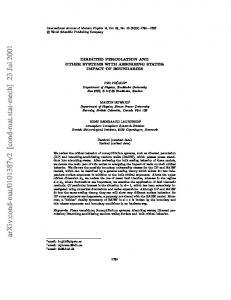
FIG. 2: Comparison between the numerical simulations of the rules in Eqs. (10)–(12) and the theoretical predictions of the probability distribution in Eq. (9) at different times and systems sizes, according to the parameters specified in the top right of the panels. The noisy lines are the numerical profiles obtained by averaging over 106 stochastic simulations. While initially fluctuations are approximately Gaussian, in the sequel they are non–Gaussian and peak at zero. In all cases ν = 0.01 and n0 = 300. (1)

(1)

where we have used that T− (0) − T+ (0) = ν and (1) (1) T− (0) + T+ (0) = 2 − ν (see Eqs. (13) and (14)). In order to test the validity of the methods, we performed extensive numerical simulations of Eqs. (10)–(12) through the Gillespie algorithm [13], which allows one to produce time series which exactly recover the solution of the master equation (1) with the rates in Eqs. (13) and (14). Fig. (1) shows typical results of the stochastic simulations and their comparison with the absorbing van Kampen solution in Eq. (16). For short times the first three profiles overlap well, but as time increases, the probability distribution does not match the numerical simulation, as shown in the last three panels. Furthermore, the agreement does not improve on increasing the size of the system. In contrast, Fig. (2) shows the solution in Eq. (9) with µ = ν and D = (2 − ν)/2. In-

creasing N , while keeping τ fixed, improves the matching as shown in the first three panels. As expected Eq. (9) converges to the numerical profiles as τ increases.

As illustrated in both figures, in the presence of an absorbing state, the system is characterized by at least two temporal scales, τ1 and τ2 , which make fluctuations evolve according to Eq. (7) for τ < τ1 and Eq. (8) for τ > τ2 . It is possible to estimate roughly the two scales by observing that one should expect the generalized van Kampen ansatz to work until the fluctuations are of the same magnitude as the macroscopic part, namely N φ(τ ) ≃ N α σ(τ ) where σ(τ ) is the variance of ξ. When pα = 1/2, this condition translates into N φ0 e−ντ ≃ 2N η(τ ) which gives τ1 ≃ 1/(3ν) ln(n0 ν/(2−ν)) for ντ ≫ 1. p For the expansion with α = 0, we have N φ0 e−ντ ≃ e−ντ (2 − ν)n0 /ν(eντ − 1) which gives τ2 ≃ 1/ν ln(νn0 /(2 − ν) + 1). Note that τ1 < τ2 . The above mentioned condition of validity of the classic van Kampen expansion is confirmed by numerical simulations (data not shown). Finally, for systems with absorbing boundaries, it is interesting to calculate an analytical expression for the survival probability PS (τ ) [14]. In our case, we get the exact n expression PS (τ ) = 1 − [(1 − e−ντ )/(1 − (1 − ν)e−ντ )] 0 which, in the scaling limit ν → 0 with ντ fixed, simplifies to f (ντ )/t with f (z) = zn0 /(ez − 1). Amazingly, the sameR result is also obtainable using Eq. (9), with PS (τ ) = dξΠ(ξ, τ |ξ0 , 0). Summarizing, in the presence of systems with absorbing states, one has to generalize the standard van Kampen ansatz in order to monitor the temporal evolution at large times. As time elapses, fluctuations become more and more important and are no longer Gaussian. However, they still can be analytically treated and lead to the general solution given by Eq. (9). Acknowledgments. We thank Duccio Fanelli for useful discussions. S. A. acknowledges the EU FP7 SCALES project (No. 26852) for financial support. The work is supported by The Cariparo foundation.

[1] C. W. Gardiner, Handbook of Stochastic Methods, 2nd (1993). ed. (Springer, 1985). [10] J. Silvertown, S. Holtier, J. Johnson, and P. Dale, Jour[2] N. G. van Kampen, Stochastic preocesses in Physics and Chemistry nal of Ecology, 80, 527 (1992). (North Holland, Amsterdam, 1992). [11] R. Durrett and S. Levin, Phil. trans. R. Soc. Lond B, [3] T. Tom´e and M. J. de Oliveira, PRE, 79, 061128 (2009). 343, 329 (1994). [4] A. J. McKane and T. J. Newman, PRL, 94, 218102 [12] T. Zillio, I. Volkov, J. R. Banavar, S. P. Hubbell, and (2005). A. Maritan, Phys. Rev. Lett., 95, 098101 (2005). [5] S. H. Lehnigk, J. Math. Phys., 19, 1267 (1978). [13] D. T. Gillespie, J. Comp. Phys., 22, 403 (1976). [6] T. M. Liggett, Interacting Particle Systems (Springer, [14] M. A. Munoz, G. Grinstein, and Y. H. Tu, PRE, 56, 5101 (1997). Berlin, 2004). [15] Suppose that f± (x) are two analytic functions such that [7] V. Sood and S. Redner, PRL, 94, 178701 (2005). f± (0) = 1, λ± two constants rates, l+ ≥ l− > 1 and [8] C. Castellano, M. A. Munoz, and R. Pastor-Satorras, that T (n ± 1|n) = λ± (n/N )l± f± (n/N ) for n/N ≪ 1. In PRE, 80, 041129 (2009). this case in Eq. (8) both the drift and diffusion terms are [9] J. W. Evans and T. R. Ray, Phys. Rev. E, 47, 1018

5 proportional to ξ l− . [16] The master equation (1) with the transition rates as given by Eqs. (13) and (14) can be analytically solved in the

infinite size limit. However the explicit solution can be numerically evaluated only at small n.