We study the response of an attractor neural network, in the ferromagnetic .... At zero temperature, the free energy has four minima, located at the corners ..... [13] Hertz J., Krogh A. and Palmer R., Introduction to the theory of neural computation.
arXiv:cond-mat/0503374v1 [cond-mat.stat-mech] 15 Mar 2005
Europhysics Letters
PREPRINT
System size resonance in an attractor neural network M. A. de la Casa 1 (∗ ), E. Korutcheva 1 (∗∗ ), J. M. R. Parrondo 2 and F. J. de la Rubia 1 1
Dpto. F´ısica Fundamental, Universidad Nacional de Educaci´ on a Distancia, c/Senda del Rey 9, 28040 Madrid, Spain 2 Grupo Interdisciplinar de Sistemas Complejos (GISC) and Dep. F´ısica At´ omica, Molecular y Nuclear, Universidad Complutense, 28040 Madrid, Spain
PACS. 05.70.Ln – Non-equilibrium and irreversible thermodynamics. PACS. 05.40.Ca – Noise. PACS. 07.05.+i – Neural networks.
Abstract. – We study the response of an attractor neural network, in the ferromagnetic phase, to an external, time-dependent stimulus, which drives the system periodically toward two different attractors. We demonstrate a non-trivial dependence of the response of the system via a system-size resonance, by showing a signal amplification maximum at a certain finite size.
Introduction. – The counter-intuitive role of fluctuations as a source of order has attracted much attention for the last years [1, 2]. Particularly interesting is the phenomenon of stochastic resonance where the response of a non-linear system to the action of a weak signal is enhanced, not hindered, by the addition of an optimal amount of noise [3]. Among several potential applications of stochastic resonance, there is evidence that it plays an important role in some cognitive processes, such as perception [4–6]. Another phenomenon that recently appeared in the literature and is closely related to stochastic resonance is system size resonance, or SSR from now on [7]. In SSR, the presence of noise in a system of finite size, close to a second-order phase transition, gives rise to the appearance of an optimal size for the system to adapt to an external field [7–9]. Inspired by the applications of stochastic resonance to cognitive processes, in this Letter we show that SSR can operate in a simple model of associative memory, namely, a Hopfield neural network [10], improving its ability to follow a time-dependent stimulus. We will focus on the simplest case of a Hopfield network storing just two patterns. Model. –
The model is defined by the following Hamiltonian [10]: H=−
X µ(t) 1 X ξi si , Jij si sj − h N i βc,r . Consequently, when the temperature increases from absolute zero the first transition occurs for the variable p, i.e., in the region of distinct bits. This means that for temperatures β ∈ [βc,r , βc,p ], the system only exhibits two minima with p = d/2, i.e., with m1 = m2 [see Eq. (5)]. One of these two minima approximately reproduces the common bits of the two patterns, whereas the distinct bits are completely disordered. The other minima is just the negative image of the first. Consequently, the system has mixed up the two patterns and it is unable to distinguish between them. The free energy landscape corresponding to this situation is plotted in Fig. 2 b). On the other hand, if d > 0, 5, the two patterns are different enough to be distinguished even for intermediate temperatures. In this case βc,r > βc,p , and the first transition occurs at βc,r . Therefore, if β ∈ [βc,p , βc,r ], we have two minima with r = (1−d)/2, i.e., with m1 = −m2 . One of the two minima reproduces the distinct bits of pattern 1 and the other one the distinct bits of pattern 2. For both minima, the common bits are disordered. Although the system does not exactly reproduce the stored patterns, it perfectly distinguish between them. The free energy in this case is plotted in Fig. 2 c). Finally, above the maximum critical temperature, the only equilibrium state is completely disordered: r = (1 − d)/2 and p = d/2, or m1 = m2 = 0, as shown in Fig. 2 d). Along this Letter we will focus only on the third case: patterns with d > 0.5 and temperatures corresponding to the landscape in Fig. 2 c). The reason is that the system still distinguish between the two patterns, but we can reach temperatures high enough to clearly observe SSR.
4
EUROPHYSICS LETTERS
b)
a) -0,35
-0,6
-0,4 -0,64 -0,45 -0,68
-0,5 -0,55
-0,72 0,3
-0,6 0,7
0,25 0,6
0,2 0,5
0,15 0,4
p
0,3
0,1 0,2
0,05 0,1
0
0,3
r
0,25
0,2
0,15
p
0
c)
0,1
0,05
0
0
0,1
0,2
0,3
0,4
0,5
0,6
0,7
r
d) -0,6
-0,6 -0,8 -0,64 -1 -0,68 -1,2 -0,72 0,3 0,25 0,7
0,6
0,2 0,5
0,15 0,4
p
0,3
0,1 0,2
0,05 0,1
0
0
r
0,3 -1,4 0,7
0,25 0,6
0,5
0,15 0,4
p
0,3
0,1 0,2
0,05 0,1
0
0,2
r
0
Fig. 2 – The free energy landscape for h = 0 and N = 10000. a) Low temperature, β = 2, d = 0.7: The free energy presents four minima, corresponding to the two stored patterns and their respective negatives. b) Medium temperature, similar patterns, β = 1, d = 0.3: There are two equilibrium states with p = d/2, i.e., with m1 = m2 . One of the minima reproduces the common bits of the two patterns whereas the other one is its negative. c) Medium temperature, dissimilar patterns, β = 1, d = 0.7: There are two equilibrium states with r = (1 − d)/2, i.e., with m1 = −m2 . Each minima reproduces the distinct bits of each pattern. d) High temperature, β = 0.5, d = 0.7: The only minimum is the disordered state with r = (1 − d)/2, p = d/2, i.e., with m1 = m2 = 0.
Results. – We have performed out-of-equilibrium Monte Carlo simulations [15] at inverse temperature β using the Hamiltonian (1). The dynamics is defined by a standard Metropolis algorithm in which 100000 sweeps have been carried out averaging over 100 realizations for every parameter set. The simulations show a clear evidence of SSR. A relevant example is presented in Fig. 3, with the distinctive features of stochastic resonance. For small N , fluctuations are strong and the system output is too noisy being unable to retrieve the patterns dynamically. The hoping between the attractors is random and not synchronized with the switches of the external stimulus. For very large N , fluctuations are weak and the system is quenched in a given attractor. However, for intermediate values of N , the system follows the oscillations of the external stimulus and the appropriate pattern for every half-period is retrieved very precisely. In order to obtain a more quantitative picture of SSR, we use the power spectrum Sm (ω) of one of the order parameters. We will focus on the power spectrum of m1 (t), but similar results are obtained if m2 (t) is chosen. A measure of the quality of the response of the system to the external input is the so-called signal amplification η [16], defined as the ratio between the power spectrum at the external frequency Ω = π/T and the total power contained in the external stimulus: R Ω+∆ω 2 Ω−∆ω Sm (ω)dω η = lim . (8) ∆ω→0 h2
M. A. de la Casa et al.: System size resonance in an attractor neural network 5
1
1
m1
a)
1
b)
0,5
0,5
0,5
0
0
0
-0,5
-0,5
-0,5
-1 300
500 t
700
-1 300
500 t
700
c)
-1 300
500 t
700
Fig. 3 – Time evolution of the order parameter m1 showing the first evidence of system-size resonance. The solid thin line is the order parameter obtained from numerical simulations. The thick segments show the time intervals in which the external stimulus drives the system to retrieve one or the other pattern. The parameters values are: β = 1.2, d = 0.6, T = 100, h = 0.01. a) N = 20; b) N = 60; c) N = 120.
Following previous work [7, 16], we will use the signal amplification η to locate and assess resonance phenomena. We have also obtained an analytical expression for Sm (ω) reproducing quite well the numerical experiments. The main idea is to approximate the dynamics of the network by a two-state system and follow the calculation performed in [3,17]. The details of the theory will be presented in a forthcoming publication [18]. Here we will only sketch the main steps of the calculation. The starting point is a master equation for the two-state system. The states are the two minima of the free energy, which are located numerically. As shown above, each of these minima reproduces fairly well the two stored patterns, hence we label them as 1 and 2. The transition probabilities between these two states W1→2 and W2→1 depend on time as W1→2 (µ(t)), µ(t) being the pattern shown to the network at time t. We have chosen an Arrhenius-like expression as in [3, 17]: W1→2 (1) = c exp(−β∆F ) exp(−βhd12 N/2) W1→2 (2) = c exp(−β∆F ) exp(βhd12 N/2),
(9)
where d12 is the difference between the values of the order parameter m1 in the two minima, ∆F is the free energy barrier separating, at zero external field, the two minima along the path r = (1 − d)/2, with m1 = −m2 , and c is an arbitrary constant (see panel c in Fig. 2). The transition probabilities Wi→j are chosen to satisfy detailed balance: W1→2 (1) = W2→1 (2). The corresponding master equation for this two-state stochastic process can be solved exactly to get the time-dependent moments < m1 (t) > and < m1 (t)m1 (t + τ ) >. Finally, by using Wiener-Khinchin theorem [19], we obtain the following explicit expression for the power spectra Sm (ω): � � �� d212 2Ω πW 2W 2 Sm (ω) = 1 − tanh (βhd12 N ) 1 − tanh( ) 2 4 πW 2Ω ω + W2 ∞ X W2 2d2 + 12 tanh2 (βhd12 N ) 2 2 π (2k − 1) (W + (2k − 1)2 Ω2 ) k=1
× (δ[ω − (2k − 1)Ω] + δ[ω + (2k + 1)Ω])
(10)
6
EUROPHYSICS LETTERS
with W = W1→2 (1) + W1→2 (2) = c exp(−β∆F ) cosh(βhdN ).
(11)
The resonant behavior of the signal amplification η can be seen in Fig. 4. There is a maximum 4000
2000
b)
1500
3000
1000
2000
η
η
a)
1000
500
0
0
100
50
0
150
0
20
40
60
N
N
Fig. 4 – The signal amplification, η, versus the size of the system, N for h = 0.01. The result of the numerical simulation is represented by dots while the analytical result is the solid line. a) d = 0.6, T = 500, β = 1.2. b) d = 0.75, T = 500, β = 1.2. For larger values of d, the maximum is shifted to the left. The only free parameter in this theory is c, which has been chosen to fit best the Monte Carlo data. In a), c = 0.44; in b), c = 0.65.
of the signal amplification at a finite size. The results of the numerical simulation (dots) correspond very well to the analytical results (solid line) given by Eq. (10). The difference between both panels of Fig. 4 is exclusively due to a difference in the value of the Hamming distance d, keeping the other parameters Ω, h and β equal. A larger value of d implies a higher energy barrier between the attractors which needs a larger noise intensity or smaller N to achieve the best resonance. Consequently, the maximum of η is shifted towards smaller N , and its maximum resonant value is reduced. Finally the dependence of η on the stimulus 150
η
100
50
0
0
0,01
0,02 Ω
0,03
0,04
Fig. 5 – The behavior of η as a function of the frequency Ω of the external stimulus shows the expected Lorentzian form, as in usual stochastic resonance. Again, the dots represent the numerical simulations and the solid line the analytical results. In this plot, d = 0.6, N = 50, β = 1.2 and h = 0.01. c=0.44, as in panel a) in Fig. 4.
frequency Ω is shown in Fig. 5. It shows the Lorentzian dependence expected in SR [3, 20]. A good agreement between theory and numerical simulations is observed as well.
M. A. de la Casa et al.: System size resonance in an attractor neural network 7
Conclusions. – In this paper we have presented numerical simulations and theoretical calculations, based on a two-state model, showing the presence of system size resonance effects in an attractor neural network. These effects are made evident by the resonant behavior of the signal amplification η as a function of the size of the system, as well as by the time evolution of the order parameters. We also point out the good agreement between analytical results and simulations. Our model shows that noise can provide the flexibility that an adaptive memory needs to follow a time-dependent stimulus. Since noise depends on the size of the system, we conclude that there is an optimal size for which there is maximal synchronization of the system to the evolving stimulus. We have explicitly shown this resonant phenomenon in a simple model with two attractors, but it is likely that more complicated models exhibit the same effect. ∗∗∗ This work is financially supported by Ministerio de Ciencia y Tecnolog´ıa (Spain), Projects No. BFM2001-291 and FIS2004-271, and by UNED, Plan de Promoci´on de la Investigaci´on 2002. REFERENCES [1] Horsthemke W. and Lefever R., Noise-induced transitions (Springer-Verlag, Berlin) 1984. [2] Garc´ıa-Ojalvo J. and Sancho J. M., Noise in spatially extended systems (Springer-Verlag, New York) 1999. ¨ nggi P., Jung P. and Marchesoni F., Rev. Mod. Phys., 70 (1998) 223. [3] Gammaitoni L., Ha [4] Riani M., Seife C., Roberts M., Twitty J., and Moss F., Phys. Rev. Lett., 78 (1997) 1186. [5] Russell D.F., Wilkens L.A., and Moss F., Nature, 402 (1999) 291. [6] Hidaka I., Nozaki D., and Yamamoto Y., Phys. Rev. Lett., 85 (2000) 3740. [7] Pikovsky A., Zaikin A. A. and de la Casa M. A., Phys. Rev. Lett., 88 (2002) 050601. [8] Toral R., Mirasso C. R. and Gunton J. D., Europhys. Lett., 61 (2003) 162. [9] Schmid G., Goychuk I., Hanggi P., Zeng S. and Jung P, Fluctuations and Noise Letters, 4 (2004) L33. [10] Hopfield J., Proc. Natl. Acad. Sci. USA, 79 (1982) 2554. [11] Hebb D., The organization of behavior: a neurophysiological theory (Wiley, New York) 1949. [12] Special issue in memory of Elizabeth Gardner, J. Phys. A: Math. Gen., 22 (1989) 19592265. [13] Hertz J., Krogh A. and Palmer R., Introduction to the theory of neural computation (Addison-Wesley, New York) 1991. [14] Privman V., Finite-size scaling and numerical simulations of statistical systems (World Scientific, Singapore) 1990. [15] Newman M. E. J. and Barkema G. T., Monte Carlo methods in statistical physics (Clarendon Press, Oxford) 1999, sect. II. ¨ nggi P., Phys. Rev. A, 44 (1991) 8032. [16] Jung P., and Ha [17] McNamara B. and Wiesenfeld K., Phys. Rev. A, 39 (1989) 4854. [18] de la Casa M. A., Korutcheva E., J.M.R. Parrondo and de la Rubia, F. J.,in preparation. [19] Gardiner C. W., Handbook of stochastic methods (Springer-Verlag, Berlin) 1983. [20] Jung P., Phys. Reports, 234 (1993) 175.