System-Wide Effectiveness of Active Learning in Collaborative Filtering Mehdi Elahi, Francesco Ricci, Valdemaras Repsys, Free University of Bozen-Bolzano Bozen-Bolzano, Italy
[email protected],
[email protected],
[email protected]
Abstract The accuracy of a collaborative-filtering system largely depends on two factors: the quality of the recommendation algorithm and the number and quality of the available product ratings. In general, the more ratings are elicited from the users, the more effective the recommendations are. However, not all the ratings are equally useful and specific techniques, which are defined as rating elicitation strategies, can be used to selectively choosing the items to be presented to the user for rating. In this paper we consider several rating elicitation strategies and we evaluate their system utility, i.e., how the overall behavior of the system changes when new ratings are added. We discuss the pros and cons of different strategies with respect to several metrics (MAE, precision, NDCG and coverage). It is shown that different strategies can improve different aspects of the recommendation quality.
1
Introduction
Choosing the right product to consume or purchase is nowadays a challenging problem due to the growing variety of eCommerce services and the informational globalization. Recommender Systems (RSs) aim at addressing this problem providing personalized suggestions for digital content, products or services, that better match the user’s needs and constraints than the mainstream products [Resnick and Varian, 1997] [Ricci et al., 2011b]. In this paper we are concerned with collaborative filtering (CF) RSs [Koren, 2008] [Li et al., 2008]. A CF system uses ratings for items provided by a population of users to predict, for a target user, what are the items with the highest ratings that he has not considered yet and recommend them to the user. The CF rating prediction accuracy does depend on the characteristics of the prediction algorithm, but also on the ratings known by the system. The more (informative) ratings are available the higher the recommendation accuracy is. Therefore, it is important to keep acquiring from the users new and useful ratings in order to maintain or improve the quality of the recommendations. In this work we concentrate on this aspect: understanding the behavior of several ratings acquisition strategies, such as “provide your ratings for these top ten
movies”. We aim at enlarging the set of available data in the optimal way for the whole system performance by asking the most useful ratings to the right users. We created a software which simulates the real process of rating elicitation in a community of users (Movielens and Netflix), the consequent rating database growth starting from a relatively small one (cold-start), and the system adaptation (retraining) to the new set of data. In this paper we define and test some “pure” strategies, i.e., implementing a single heuristic, but also strategies that we call “partially randomized”, which, in addition to asking to the (simulated) users to rate the items selected by a “pure” strategy, they ask to rate some randomly selected items as well. Randomized strategies can introduce diversity in the item list presented to the user But, more importantly, they have been introduced to cope with the non monotonic behavior of the system effectiveness that we observed during the simulation of certain “pure” strategies. In fact, we have discovered (as hypothesized by [Rashid et al., 2002]) that certain strategies, for instance, requesting to rate the items with the largest predicted ratings, may generate a system-wide bias, and ultimately the addition of the ratings proposed by these strategies can increase, rather than decrease, the system error. In these simulations we used a state of the art Matrix Factorization rating prediction algorithm [Koren and Bell, 2011] [Timely Development, 2008]. Hence the results here presented can provide useful guidelines for managing real RSs that nowadays largely rely on that technique. Rating elicitation has been also tackled in a few previous works [Sean M. McNee and Riedl, 2003; Rashid et al., 2002; Carenini et al., 2003; Jin and Si, 2004; Harpale and Yang, 2008] but these papers focused on a different problem, namely the benefit of the rating elicitation process for a single user, e.g., in the sign up stage [Rashid et al., 2002]. Conversely, we consider the impact of an elicitation strategy on the system-wide behavior, e.g., the overall prediction accuracy (more details are provided in section 6). In general, rating elicitation has been ignored by the mainstream RSs research. A possible explanation is because of the erroneous assumption that a RS cannot control what items the users will rate. Actually this is not true, surely RSs user interfaces can be designed so that users navigating through the existing items can rate them if they wish. But new ratings can also be acquired by explicitly asking users. In fact, it is common
practice for RSs to ask the users to rate the recommended items: mixing recommendation with users’ preferences elicitation. We will show that this approach has a potentially dangerous impact on the system effectiveness, hence a careful selection of the elicitation strategy is in order. The main contribution of our research is the introduction and empirical evaluation of a set of rating elicitation strategies for collaborative filtering with respect to their system-wide utility. Some of these strategies are new and some come from the literature and the common practice. Another important contribution of this paper is due to the fact that we measured the effect of each strategy on several RSs evaluation measures showing that the best strategy depends on the evaluation measure. Previous works focussed only on the rating prediction accuracy (Mean Absolute Error), and on the number of acquired ratings. We analyze those aspects, but in addition we consider the recommendation precision, the coverage and the goodness of the recommendations’ ranking, measured with normalized discounted cumulative gain (NDCG). These measures are more interesting and useful for determining the true value of the recommendations for the user. Moreover, in our work we explore another new aspect, i.e., the performance of the elicitation strategies taking into account the size of the rating database and we show that different strategies can improve different aspects of the recommendation quality at different stages of the rating database development. In fact, we show that in some stages an elicitation strategy may induce a bias on the system and ultimately a decrease of the recommendation effectiveness. In addition, previously conducted evaluations assume rather artificial conditions, i.e., that all the users and the items have some ratings since the beginning of the evaluation process. In other words, they did not faced the new-item and the new-user problem). We instead generate initial conditions for the rating data set in a pure random way, hence, in our experiments, new users and new items are present as it happens in real conditions. In conclusion in this paper we provide a realistic, comprehensive evaluation of several applicable rating elicitation strategies, providing guidelines and conclusions that would help their exploitations in real RSs. The rest of the paper is structured as follow. In section 2 we introduce the rating elicitation strategies that we have analyzed, and in section 3 we present the simulation procedure that we designed to evaluate their effects. The results of our experiments are shown in section 4. In section 6 we review some related researches, and finally in section 7 we summarize the results of this research and we outline some future work.
2
Elicitation Strategies
A rating dataset R is a n × m matrix of real values (ratings) with possible null entries. The variable rui , denotes the entry of the matrix in position (u, i), and contains the rating assigned by user u to item i. rui could store a null value representing the fact that the system does not know the opinion of the user on that item. In the Movielens and Netflix datasets the rating values are integers between 1 and 5 included. A rating elicitation strategy S is a function S(u, N, K, Uu ) = L which returns a list of items L = {i1 , . . . , iM } whose rat-
ings should be asked to the user u, where N is the maximum number of ratings to be elicited, K is the dataset of known ratings, i.e., the ratings (of all the users) that have been already acquired by the RS. K is also a n × m matrix containing entries with real or null values. The not null entries represent the knowledge of the system at a certain point of the RS evolution. Finally, Uu is the set of items whose ratings have not yet requested to u, hence potentially interesting. Hence one must enforce that L ⊂ Uu and an elicitation strategy will not ask to a user to rate two times the same item; hence the items in L, which are returned by S, must be removed from Uu . Every strategy analyzes the dataset of known ratings K and assigns a score to the items in Uu . Then the N items with the highest score are returned, if the strategy can score N different items, otherwise a smaller number of items is returned. It is important to note that the user may have not experienced the items whose ratings are requested; in this case the system will not increase the number of known ratings. Some strategies may collect more ratings, some strategies may be better in collecting useful ratings. These two properties play a fundamental role in a rating elicitation strategy.
2.1
Individual Strategies
We considered two types of strategies: pure and partially randomized. The first ones implement a unique heuristic, whereas in the second type of strategies a pure one is hybridized by adding some random rating requests that are still unclear to the system. As we mentioned in the introduction these strategies add some diversity to the system requests and, as we will show later, can cope with an observed problem of pure strategies: they may in some cases increase the system error. The pure strategies that we considered are: • Popularity: for all the users the score for item i is the number of not null ratings for i contained in K. These are the known ratings for the item i. More popular items are more likely to be known by the user, and hence it is more likely that a request for such a rating will really increase the size of the rating database. • Binary Prediction: the matrix K is transformed in a matrix B with the same number of rows and columns, by mapping null entries in K to 0, and not null entries to 1. A factor model is built using the matrix B as training data, and then a prediction for each entry in B is computed. Finally, the score for the item i in Uu is the predicted value for the entry in position (u, i) in B. This strategy tries to predict what items the user has experienced, in order to maximize the probability that the user know the requested rating (similarly to the popularity strategy). • Highest Predicted: a prediction is computed for all the items in Uu and the scores are set equal to these predicted values. The idea is that the best recommendations could also be more likely to have been experienced by the user and their ratings could also reveal more information on what the user likes. Moreover, this is the default strategy for RSs, i.e., enabling the user to rate the recommendations.
• Lowest Predicted: for all the items in Uu a prediction rˆui is computed. Then the score for i is M axr − rˆui , where M axr is the maximum rating value (e.g., 5). Lowest predicted items are likely to reveal what the user does not like, but are likely to collect a few ratings, since the user is unlikely to have experienced all the items that he does not like. • Highest and Lowest Predicted: for all the items in Uu a prediction rˆui is computed. The score for an item is inr | M axr−M + M inr − rˆui |, where M inr is the min2 imum rating value (e.g., 1). This strategy tries to ask ratings for items that the user may like and not like as well. • Random: the score for an item is a random integer number from 1 to 10. This is just a baseline strategy, used for comparison. • Variance: the score for the item i is equal to the variance of its ratings in the dataset K. This is a representative of the strategies that try to collect more useful ratings, assuming that the opinion of the user on items with more diverse ratings are more useful to the generation of correct recommendations.
2.2
Partially Randomized Strategies
In a partially randomized strategy we modify the list of items returned by a pure strategy introducing some random items. As we mentioned in the introduction, these strategies have been introduced to cope with some problems of the pure ones (see section 4). Precisely, the randomized version Ran of the strategy S with randomness p ∈ [0, 1] is a function Ran(S(u, N, K, Uu ), p) returning a new list of items L0 computed as follow: 1. L = S(u, N, K, Uu ) is obtained 2. if L is an empty list, i.e., the strategy S for some reason could not generate the elicitation list, then L0 is computed by taking N random items from Uu . 3. if |L| < N , L0 = L ∪ {i1 , . . . , iN −|L| }, where ij is a random item in Uu . 4. if |L| = N , L0 = {l1 , . . . , lM , iM +1 , . . . , iN }, where lj is a random item in L, M = dN ∗ (1 − p)e, and ij is a random item in Uu . We note that if S is the highest predicted strategy, there are cases where no rating predictions can be computed by the RS for the user u, and hence S is not able to sort the items to request. This happens for instance when u is a new user and none of his ratings is known. In this case the randomized version of this strategy generates purely random items for the user to rate.
3
Evaluation Approach
In order to study the effect of the considered elicitation strategies we set up a simulation procedure. The goal was to simulate the evolution of a RS’s performance exploiting these strategies. In order to run such simulations we partition all the available (not null) ratings in R into three different matrices with the same number of rows and columns as R:
• K: contains the ratings that are considered to be known by the system at a certain point in time. • X: contains the ratings that are considered to be known by the users but not by the system. These ratings are incrementally elicited, i.e., they are transferred into K if the system asks them to the (simulated) users. • T : contains the ratings that are never elicited and are used only to test the strategy, i.e., to estimate the evaluation measures (defined later). We also note that Uu is the set of items whose ratings, at a certain point in time, are worth acquiring because “unclear” to the system. That means that kui has a null value and the system has not yet asked it to u. That request may end up with a new (not null) rating kui inserted in K, if the user has experienced the item i, i.e., if xui is not null, or in a no action, if xui has a null value in the matrix X. The system, in any case will remove the item i from Uu , to not ask twice the same rating. We will discuss later how the simulation is initialized, i.e., how the matrices K, X and T are built from the full rating dataset R. In any case, these three matrices partition the full dataset R; if rui has a not null value then either kui or xui or tui has that value, and only one of them is not null. The testing of a strategy S proceeds in the following way: 1. The not null ratings in R are partitioned into the three matrices K, X, T . 2. MAE, Precision and NDCG are measured on T , training the rating prediction model on K. 3. For each user u: (a) Only the first time that this step is executed, Uu , the unclear set of user u is initialized to all the items i with a null value kui in K. (b) Using strategy S (pure or randomized) a set of items L = S(u, N, K, Uu ) is computed. (c) The set Le , containing only the items in L that have a not null rating in X, is created. (d) Assign to the corresponding entries in K the ratings for the items in Le as found in X. (e) Remove the items in L from Uu : Uu = Uu \ L. 4. MAE, Precision and NDCG are measured on T , and the prediction model is re-trained on the new set of ratings contained in K. 5. Repeat steps 3-4 (Iteration) for I times. The MovieLens [Miller et al., 2003] and Netflix rating databases were used for our experiments. Movielens consists of 100,000 ratings from 943 users on 1682 movies. From the full Netflix data set, which contains 1,000,000 ratings, we extracted the first 100,000 ratings entered into the system. They come from 1491 users on 2380 items, so this sample of Netflix data is 2.24 times sparser than Movielens data. We also performed some experiments with the larger versions of of both Movielens and Netflix datasets (1,000,000 ratings) and obtained very similar results. However, using the full set of Netflix data required much longer times to perform our experiments since we train and test a rating prediction
model at each iteration: every time we add to K new ratings elicited from the simulated users. After having observed a very similar performance on some initial experiments we focussed on the smaller data sets to be able to run more experiments. When deciding how to split the available data into the three matrices K, X and T an obvious choice is to respect the time evolution of the dataset, i.e., to insert in K the first ratings acquired by the system, then to use a second temporal segment to populate X and finally use the remaining ratings for T . Actually, it is not significant to test the performance of the proposed strategies for a particular evolution of the rating dataset. Since we want to study the evolution of a rating data set under the application of a new strategy we cannot test it only against the temporal distribution of the data that was generated by a particular (unknown) previously used elicitation strategy. Hence we followed the approach used in [Harpale and Yang, 2008] to random split the rating data, but we generated several random splits of the ratings into K, X and T . Besides, in this way we could generate ratings configurations where there are users and items that have no (not null) ratings initially in the known dataset K. We believe this approach provided us with a very realistic and hard experimental setup, letting us to address the new user and new item problems [Ricci et al., 2011a]. Finally, we observe that for both data sets the experiments were conducted partitioning (randomly) the 100,000 not null ratings of R in the following way: 2000 in K (i.e., very limited knowledge at the beginning), 68,000 in X, and 30,000 in T . Moreover, |L| = 10, which means that the system at each iteration asks to a user his opinion on 10 items. The number of iterations was I = 170, and the number of factors in the SVD prediction model was set to 16. All the experiments were performed 5 times and results presented in the following section are obtained as averages of these five repetitions. We considered four evaluation measures: mean absolute error (MAE), precision, coverage and normalized discounted cumulative gain (NDCG) [Herlocker et al., 2004; Manning, 2008]. For computing precision we extracted, for each user, the top 10 recommended items (whose ratings appear in T ) and considered as relevant the items with true ratings equal to 4 or 5. The coverage of a recommender system is measured as the proportion of the full set of items over which the system can form predictions [Herlocker et al., 2004]. Discounted cumulative gain (DCG) is a measure originally used to evaluate effectiveness of information retrieval systems [J¨arvelin and Kek¨al¨ainen, 2002], but also collaborative filtering RSs [Weimer et al., 2008] [Liu and Yang, 2008]. In RSs the relevance is measured by the rating value of the item in the predicted recommendation list. Assume that the recommendations for u are sorted according to the predicted rating values, then DCGu is defined as: DCGu =
N X i=1
rui log2 (i + 1)
(1)
where rui is the true rating (as found in T ) for the item ranked in position i for user u, and N is the length of the recommendation list. Normalized discounted cumulative gain
for user u is then calculated in the following way: DCGu (2) IDCGu where IDCGu stands for the maximum possible value of DCGu , that could be obtained if the recommended items are ordered by decreasing value of their true ratings. We measured also the overall average discounted cumulative gain N DCG by averaging N DCGu over the full population of users. N DCGu =
4
Evaluation of Pure Strategies
4.1
MAE
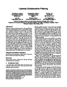
The MAE computed on the test matrix T at successive iterations of the application of the elicitation strategies is depicted in Figure 1. First of all we must observe that the behavior of the considered strategies in the two data sets are very similar. Moreover, there are two clearly distinct groups: 1. Monotone error decreasing strategies: lowest-highest predicted, lowest predicted and random. 2. Non-monotone error decreasing strategies: binary predicted, highest predicted, popularity, variance. Strategies of the first group show an overall better performance (MAE) for all the duration of the test except at the beginning and the end. During the iterations 1-5 the best performing strategy is binary-predicted, the second best being highest predicted, both being non-monotone. During iterations 6-45 random strategy has the lowest MAE value in the Movielens data set, and it is overtaken by the lowest-highestpredicted strategy at iteration 46. This is not observed in the Netflix data set. At the iteration 80 the MAE obtained using the variance, popularity and all the prediction-based strategies stop changing: as K reaches the largest possible size for those strategies. The MAE obtained using the random strategy keeps decreasing until all the ratings in X are moved to K. It is important to note that the prediction based strategies (e.g., highest predicted) cannot elicit ratings for which the prediction can not be made, i.e., for all those movies and users that don’t have (not null) ratings in K. This is reflected by the behavior of the coverage The coverage graph is not shown here for lack of space, but we can summarize these results noting that the coverage of the prediction-based strategies is stable, with value 0.74 (Movielens) throughout the experiment, because the set of users or items with not null ratings in K is not increasing. The system coverage produced by the random strategy is slowly increasing and reaches the full coverage, because ratings for new users and new items are randomly added to K. The coverage obtained by the variance and popularity strategies increases and stabilizes to 0.84 on iteration 10, but it does not reach the full coverage. This is because those strategies are able to elicit ratings from new users, but are not able to elicit ratings for new items. Very similar results are observed in the Netflix data. The non-monotone strategies’ behaviors can be divided into three stages: they decrease MAE at the beginning (approximately iterations 1-5), then they slowly increase it, when MAE reaches a peek (approximately iterations 6-35), and
(a) Movielens
(b) Netflix
Figure 1: MAE of the pure strategies
Table 1: The percentage of the ratings elicited by the Highest Predicted strategy at different iterations Iterations 1 to 5 35 to 40
r=1 2.06% 6.01%
Percentage of elicited ratings (r) r=2 r=3 r=4 r=5 4.48% 16.98% 36.56% 39.90% 13.04% 29.33% 34.06% 17.53%
then they slowly decrease MAE till the end of the experiment (approximately iterations 36-80). The explanation of such a behavior is that the strategies belonging to this second group have a selection bias which can negatively affects MAE. For instance, the highest predicted strategy at the first iterations elicits many more high ratings compared to those elicited later on (Table 1). As a result it ends up with adding more high (than low) ratings to the known matrix (K), which biases the rating prediction. In fact, low rated movies are selected for elicitation by the highest predicted strategy in two cases: 1) when a low rated item is predicted to have a high rating 2) when all the highest predicted ratings have been already elicited or marked as “not available” (they are not present in X and removed from Uu ). Looking into the data we discovered that at iteration 36 the highest-predicted strategy has already elicited most of the highest ratings. Then the next ratings that are elicited are actually average or low ratings, which reduces the bias in K and also the prediction error. The random and lowest-highest predicted strategies do not introduce such a bias, and this results in a constant decrease of MAE.
4.2
Number of Acquired Ratings
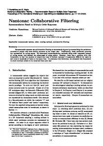
It is important to measure how many ratings are added by the considered strategies. In fact, certain strategies can acquire
more ratings by better guessing what items the user actually experienced. This occurs in our simulation if a strategy asks to the simulated user more ratings that are present in the matrix X. Conversely, a strategy may not be able to acquire many ratings but those actually acquired are very useful to generate better recommendations. Figure 2 shows the size of the system known ratings in K, as the strategies elicit new ratings from the simulated users. It is worth noting, even in this case, the strong similarity of the behavior of the considered strategies in the two data sets. The only strategy that differs substantially in the two data sets is random. This is clearly dependent on the larger number of users and items that are present in our sample of the Netflix data. In fact, here there are 100,000 ratings as in the Movielens data set but the sparsity is higher: there are only 2.8% of the possible ratings (1491*2380) vs. 6.3% of the possible ratings (943*1682) contained in the Movielens data set. This larger sparsity makes more difficult for a pure random selection to pick up items that are known to the user. In general this is a major limitation of any random strategy, i.e., the very slow rate of addition of new ratings. Hence for relatively small problems (items and users) the random strategy may be applicable, but for larger ones this is impractical. In fact, observing Figure 2, one can see that in the Movielens simulations after 70 iterations, which means 70*10*943=660.100 ratings’ requests (iterations * numberof-rating-requests * users) the system has acquired on average only 28.000 new ratings (30.000 is the new size but 2000 were already present at the beginning of the process). This means that only one out of 23 random rating requests could be provided by a user. In the Netflix data set this is even worse. It is interesting to note that even the popularity strategy has a
(a) Movielens
(b) Netflix
Figure 2: Number of elicited ratings poor performance in term of number of elicited ratings; it can elicit the first 28.000 ratings at a speed equal to one rating for each 6.7 rating requests. We also observe that according to our results, quite surprisingly the larger sparsity of the Netflix sample has produced a substantially different impact only on the random strategy. Figure 3 illustrates a related aspect, i.e., how much the acquired ratings are useful for the effectiveness of the system, i.e., how the same number of ratings, acquired by different strategies can reduce MAE. It is clear that in the first stage of the process, i.e., when a small number of ratings are present in the known set K, the random and lowestpredicted strategies collect the more useful ratings for reducing MAE. Successively, the lowest-highest-predicted strategy bring more useful ratings. This is an interesting result, showing that the items with the lowest predicted ratings and random items are bringing more useful information even if it is difficult to acquire these ratings. It is also clear that certain strategies are not able to acquire all the ratings in X. For instance lowest-highest-predicted, lowest-predicted and highest-predicted stop acquiring new ratings when they have collected 50.000 ratings (Movielens). This is due to the fact that these strategies need rating predictions that in some cases (e.g., for new users) cannot be made by the system.
4.3
NDCG
We measured NDCG on the first top 10 recommendations with not null values in T (for each user) (Figure 4). Note that sometime we computed NDCG on a smaller set, i.e., only on the ratings in the user test set whose value can be actually predicted. Popularity is the best strategy at the beginning of the experiment. But at iteration 4 (Movielens) and 15 (Netflix) the ran-
dom strategy passes the popularity strategy and then remains the best one. Excluding the random strategy, popularity and variance are the best in both data sets. Lowest predicted is by far the worst, and this is quite surprising considering how effective it is in reducing MAE. Moreover, another striking difference from the MAE results, is that all the strategies improve NDCG monotonically. Analyzing the experiment data we discovered that lowest predicted is not effective for NDCG because it is eliciting more ratings for the lowest ranked items and this is useless to predict the ranking of the top items. It is also important to note that here the random strategy is by far the best. This is again different from the MAE behavior.
4.4
Precision
In the rest of this paper we focus on the Movielens data. In fact, as we have already observed apropos of MAE and NDCG, very similar results were observed for the system precision using the Netflix data, so for lack of space we omit them. Precision, as it was described in section 3, measures the proportion of items rated 4 and 5 that are found in the recommendation list. Figure 5 depicts the evolution of the system precision when the proposed strategies are applied. Here, highest predicted is the best performing strategy for the largest part of the test. Starting from iteration 50 it is equally good as the binary predicted and the lowest-highest-predicted strategies. It is also interesting to note that all the strategies monotonically increase the precision. Moreover, the random strategy, differently from NDCG, does not perform so well, if compared with the highest predicted strategy. This is again related to the fact that the random strategy increases substantially the coverage and this produces a lower overall precision because precision is significantly smaller for new users.
(a) Movielens
(b) Netflix
Figure 3: MAE vs number of ratings elicited
(a) Movielens
(b) Netflix
Figure 4: NDCG of the pure strategies
(which is not the case if the goal is to improve MAE). It is important to note that the strategies that show good performance at the beginning (partially randomized highest and binary predicted strategies) are those tuned for finding items that a user may know and be able to provide a rating for. Therefore, they are very effective in the beginning when there are many users with very little items in the known dataset K.
6
Figure 5: Precision of pure strategies (Movielens) In conclusion from these experiments one can conclude that there is no single best strategy, among those that we evaluated, that dominates the others for all the evaluation measures. The random strategy is the best for NDCG, whereas for MAE and precision we would suggest using lo-high predicted, performing quite well for both measures.
5
Evaluation of the Partially Randomized Strategies
Among the pure strategies only the random one is able to elicit ratings for items that have not been evaluated by any user already represented in K. Partially randomized strategies address this problem by asking new users to rate random items (see Section 2). In this section we have used partially randomized strategies where p = 0.2, i.e., at least 2 of the 10 rating values elicited from the simulated users are chosen at random. Figure 6 depicts the system MAE evolution during the experimental process. Now all the curves are monotone, i.e., it is sufficient to add some randomly selected ratings to the elicitation lists to reduce the bias of the pure, prediction-based, strategies. The best performing partially randomized strategies, with respect to MAE, are, at the beginning of the process, the partially randomized binary-predicted, and subsequently the low-high-predicted (similarly to the pure strategies case). For lack of space, the behaviors of the system precision and NDCG are not shown here, we just describe them. These two measures behave similarly. The partially randomized highest predicted strategy has the best results for the largest part of the test (for both measures). Interestingly, the worst strategy is the lowest-predicted, i.e., it seems that for improving the recommender precision it does not pay off to ask the user his opinion on items that the system believes are irrelevant
Related Work
The rating elicitation problem can be considered as an active learning problem. Active learning aims at actively acquiring training data to improve the output of the recommender system [Rubens et al., 2011]. [Rashid et al., 2002] proposes six techniques that collaborative filtering recommender systems can use to learn about new users in the sign up process. They considered: pure entropy, i.e., items with the largest entropy are preferred; random selection; popularity, i.e., the items that have the largest number of ratings; items with the largest log(popularity) ∗ entropy, i.e., items that are both popular and have diverse rating values; and finally in “itemitem personalized” the items are proposed randomly until one rating is acquired, then a recommender is used to predict the items that the user is likely to have seen. They studied the behavior of an item-based CF only with respect to MAE, and designed an offline experimental study that simulates the sign up process. Each strategy was used to select a certain number of items (30, 45, 60 and 90) for a user without knowing if they were experienced by that user, i.e., their ratings were present in the dataset or not. Then MAE was measured for the user on the remaining ratings while using the elicited ratings, and the ratings of other training users, as training data. The process was repeated and averaged for all the test users. In this scenario the log(popularity) ∗ entropy strategy is the best. However, popularity and item-item personalized strategies outperformed log(popularity)∗entropy with respect to the user effort. User effort was computed as a fraction of items elicited over total number of items presented. It is worth noting that these results are not comparable with ours as they measured how a varying set of ratings elicited from one user are useful in predicting the ratings of the same user. In our experiments we simulate the simultaneous acquisition of ratings from all the users, by asking in turn to each user 10 ratings, and repeating this process several times. This simulates the long term usage of a recommender system where users come again and again to get new recommendations and the rating provided by a user is exploited to generate better recommendations to others (system performance). [Harpale and Yang, 2008] remarks that the Bayesian active learning approach introduced in [Jin and Si, 2004] makes an implicit and unrealistic assumption that a user can provide rating for any queried item. Hence, they propose a revised Bayesian selection approach, which does not make such an assumption, and introduces an estimation of the probability that a user has consumed an item in the past and is able to provide a rating. Their results show that the personalized Bayesian selection outperforms Bayesian selection and the random strategy
Also in this case, their results are complementary to our findings, since the elicitation process and the evaluation metrics are different.
7
Figure 6: MAE of partially randomized strategies (Movielens) with respect to MAE. Their simulation setting is similar to that used in [Rashid et al., 2002], hence for the same reason their results are not directly comparable with ours. There are other important differences between their experiment and ours: their strategies elicit only one rating per request; they compare the proposed approach only with the random strategy; they do not consider the new user problem, since in their simulations all the users have 3 ratings at the beginning of the experiment, whereas in our experiments, there might be users that have no ratings at all in the initial stage of the experiment; they use a completely different rating prediction algorithm (Bayesian vs. Matrix Factorization). All these differences make the two set of experiments hard to compare. Moreover, their simulations starts from a known ratings data set that is larger than ours. In fact, the MAE they measured initially on Movielens is around 0.83, whereas in our experiments the MAE is almost 1. In [Carenini et al., 2003] again a user-focussed approach is considered. They propose a set of techniques to intelligently select ratings when the user is particularly motivated to provide such information. They present a conversational and collaborative interaction model which elicits ratings so that the benefit of doing that is clear to the user, thus increasing the motivation to provide a rating. Item-focused techniques that elicit ratings to improve the rating prediction for a specific item are proposed. Popularity, entropy and their combination are tested, as well as their item focused modifications. The item focused techniques are different from the classical ones in that popularity and entropy are not computed on the whole rating matrix, but only on the matrix of user’s neighbors that have rated an item for which the prediction accuracy is aimed at being improved. Results have shown that item focused strategies are constantly better than unfocused ones.
Conclusions and Future Work
In this work we have addressed the problem of selecting items to present to the users for acquiring their ratings; that is also defined as the ratings elicitation problem. We have proposed and evaluated a set of ratings elicitation strategies. Some of them have been proposed in a previous work [Rashid et al., 2002] (popularity, random, variance), and some, which we define as prediction-based strategies, are new: binary-prediction, highest-predicted, lowest-predicted, highest-lowest-predicted. Moreover, we have studied the behavior of other novel strategies, partially randomized, which insert some random ratings in the elicitation lists computed by the aforementioned strategies. We have evaluated these strategies for their system-wide effectiveness implementing a simulation loop that models the day-by-day process of rating elicitation and rating database growth. We have taken into account the limited knowledge of the users, i.e., the fact that the users will not know all the possible ratings. During the simulation we have measured several metrics at different phases of the rating database growth. The metrics include: MAE to measure the improvements in prediction accuracy, precision to measure the relevance of recommendations, normalized discounted cumulative gain (NDCG) to measure the quality of produced ranking and coverage to measure the proportion of items over which the system can form predictions. The evaluation has shown that different strategies can improve different aspects of the recommendation quality and in different stages of the rating database development. Moreover, we have discovered that some pure strategies may incur in the risk of increasing the system MAE if they keep adding only ratings with a certain value, e.g., the largest ones, as for the highest-predicted strategy that is an approach often adopted in real RSs. In addition, prediction-based strategies neither address the problem of new users, nor of new items. Popularity and variance strategies are able to select items for new users, but can not select items that have no ratings. Partially randomized strategies, have less problems because they add random items to rate that have no ratings at all. In this case the lowest-highest (highest) predicted is a good alternative if MAE (precision) is the target effectiveness measure. These strategies simulate that some items to rate are deliberately selected by the user, but one can also implement this in a pure elicitation strategy because of the benefits it produces. This research opened a number of new problems that would definitely deserve some more study. First of all, it would be useful to repeat the same experiments using even more diverse datasets to study how the data distribution influences the strategies’ behavior. In fact, we have already observed that the performance of some strategies (random) depends on the sparsity of the rating data. The MovieLens data and the Netflix sample that we used, still have a considerably low sparsity compared to other larger datasets. For example, if the data sparsity was higher, there would be only a very low
probability for random strategy to select an item that a user has consumed in the past and can provide a rating for. So the partially randomized strategies may perform worse in reality or it could be needed a different degree of randomness. Furthermore, there remain many unexplored possibilities for combining strategies that use different approaches depending on the state of the target user. For instance, asking users to rate popular items when a user does not have any ratings yet and using another strategy at a latter stage. Moreover, it is important to consider the noise and inconsistency of the data when designing strategies that search for items that optimally combine the probability that a user has experienced them, and thus can really provide a rating value for them, with the usefulness of obtaining that information.
References [Carenini et al., 2003] Giuseppe Carenini, Jocelyin Smith, and David Poole. Towards more conversational and collaborative recommender systems. In Proceedings of the 2003 International Conference on Intelligent User Interfaces, January 12-15, 2003, Miami, FL, USA, pages 12– 18, 2003. [Harpale and Yang, 2008] Abhay S. Harpale and Yiming Yang. Personalized active learning for collaborative filtering. In SIGIR ’08: Proceedings of the 31st annual international ACM SIGIR conference on Research and development in information retrieval, pages 91–98, New York, NY, USA, 2008. ACM. [Herlocker et al., 2004] Jonathan L. Herlocker, Joseph A. Konstan, Loren G. Terveen, and John T. Riedl. Evaluating collaborative filtering recommender systems. ACM Trans. Inf. Syst., 22(1):5–53, 2004. [J¨arvelin and Kek¨al¨ainen, 2002] Kalervo J¨arvelin and Jaana Kek¨al¨ainen. Cumulated gain-based evaluation of ir techniques. ACM Trans. Inf. Syst., 20(4):422–446, 2002. [Jin and Si, 2004] Rong Jin and Luo Si. A bayesian approach toward active learning for collaborative filtering. In UAI ’04, Proceedings of the 20th Conference in Uncertainty in Artificial Intelligence, July 7-11 2004, Banff, Canada, pages 278–285, 2004. [Koren and Bell, 2011] Yehuda Koren and Robert Bell. Advances in collaborative filtering. In Francesco Ricci, Lior Rokach, Bracha Shapira, and Paul Kantor, editors, Recommender Systems Handbook, pages 145–186. Springer Verlag, 2011. [Koren, 2008] Yehuda Koren. Factorization meets the neighborhood: a multifaceted collaborative filtering model. In KDD ’08: Proceeding of the 14th ACM SIGKDD international conference on Knowledge discovery and data mining, pages 426–434, New York, NY, USA, 2008. ACM. [Li et al., 2008] Ying Li, Bing Liu, and Sunita Sarawagi, editors. Proceedings of the 14th ACM SIGKDD International Conference on Knowledge Discovery and Data Mining, Las Vegas, Nevada, USA, August 24-27, 2008. ACM, 2008.
[Liu and Yang, 2008] Nathan N. Liu and Qiang Yang. Eigenrank: a ranking-oriented approach to collaborative filtering. In SIGIR ’08: Proceedings of the 31st annual international ACM SIGIR conference on Research and development in information retrieval, pages 83–90, New York, NY, USA, 2008. ACM. [Manning, 2008] Christopher Manning. Introduction to Information Retrieval. Cambridge University Press, Cambridge, 2008. [Miller et al., 2003] Bradley N. Miller, Istvan Albert, Shyong K. Lam, Joseph A. Konstan, and John Riedl. Movielens unplugged: experiences with an occasionally connected recommender system. In IUI ’03: Proceedings of the 8th international conference on Intelligent user interfaces, pages 263–266, New York, NY, USA, 2003. ACM. [Rashid et al., 2002] Al Mamunur Rashid, Istvan Albert, Dan Cosley, Shyong K. Lam, Sean M. Mcnee, Joseph A. Konstan, and John Riedl. Getting to know you: Learning new user preferences in recommender systems. In Proceedings of the 2002 International Conference on Intelligent User Interfaces, IUI 2002, pages 127–134. ACM Press, 2002. [Resnick and Varian, 1997] Paul Resnick and Hal R. Varian. Recommender systems. Commun. ACM, 40(3):56–58, 1997. [Ricci et al., 2011a] Francesco Ricci, Lior Rokach, and Bracha Shapira. Introduction to recommender systems handbook. In Francesco Ricci, Lior Rokach, Bracha Shapira, and Paul Kantor, editors, Recommender Systems Handbook, pages 1–35. Springer Verlag, 2011. [Ricci et al., 2011b] Francesco Ricci, Lior Rokach, Bracha Shapira, and Paul B. Kantor, editors. Recommender Systems Handbook. Springer, 2011. [Rubens et al., 2011] Neil Rubens, Dain Kaplan, and Masashi Sugiyama. Active learning in recommender systems. In Francesco Ricci, Lior Rokach, Bracha Shapira, and Paul Kantor, editors, Recommender Systems Handbook, pages 735–767. Springer Verlag, 2011. [Sean M. McNee and Riedl, 2003] Joseph A. Konstan Sean M. McNee, Shyong K. Lam and John Riedl. Interfaces for eliciting new user preferences in recommender systems. In User Modeling 2003, 2003. [Timely Development, 2008] LLC Timely Development. Netflix prize, 2008. http://www.timelydevelopment.com/demos/NetflixPrize.aspx. [Weimer et al., 2008] Markus Weimer, Alexandros Karatzoglou, and Alex Smola. Adaptive collaborative filtering. In RecSys ’08: Proceedings of the 2008 ACM conference on Recommender systems, pages 275–282, New York, NY, USA, 2008. ACM.