repeat some process a set number of times cumsum() produce running total of values for input vector ecdf() builds empiri
Table of Useful R commands Command
Purpose
help() example() c(), scan() seq() rep() ) hist(faithful$eruptions, freq=F, n=15, main="Histogram of Old Faithful Eruption Times", xlab="Duration (mins)")
0.4 0.2 0.0
Density
0.6
Histogram of Old Faithful Eruption Times
1.5
2.0
2.5
3.0
3.5
4.0
Duration (mins)
3
4.5
5.0
R Commands for MATH 143
Examples of usage
library(), require() > library(abd) > require(lattice)
histogram() require(lattice) , xlab="Length") histogram(~ Sepal.Length | Species, ) histogram(~ Sepal.Length | Species, , header=T)
mean(), median(), summary(), var(), sd(), quantile(), > counties=read.csv("http://www.calvin.edu/~stob/) barplot(table(pol$Political04), horiz=T) barplot(table(pol$Political04),col=c("red","green","blue","orange")) barplot(table(pol$Political04),col=c("red","green","blue","orange"), names=c("Conservative","Far Right","Liberal","Centrist"))
Conservative
Liberal
Centrist
60
barplot(xtabs(~sex + Political04, ) boxplot(Sepal.Length ~ Species, , ylab="Sepal length",main="Iris Sepal Length by Species")
6.5 5.5
●
4.5
Sepal length
7.5
Iris Sepal Length by Species
setosa
versicolor
virginica
plot()
90
Old Faithful Eruptions ● ● ● ● ● ● ●● ● ● ● ● ● ● ● ● ● ● ● ● ● ●● ● ● ● ● ●● ●●●● ●● ● ● ● ● ● ● ● ●● ● ●● ●●●●●● ● ●● ●● ● ● ● ● ● ● ● ●● ● ● ● ● ●● ● ● ● ● ●● ● ●● ●● ●● ●●● ● ●● ● ●●●●●●●● ● ● ●● ● ● ● ● ● ● ● ● ● ●● ● ● ● ●● ● ● ● ● ● ●●● ●● ● ● ● ● ● ● ● ● ●●● ● ● ● ● ● ● ●● ● ● ● ●
● ● ●
●
70
● ● ●
50
Time between eruptions
) plot(waiting~eruptions, , main="Old Faithful Eruptions", ylab="Wait time between eruptions", xlab="Duration of eruption")
●
1.5
●
●
● ● ● ● ● ●● ●● ●
● ● ● ●● ●● ● ●●● ● ●●● ●● ● ● ●● ● ●●●●● ● ●●● ● ●● ● ●● ●● ●● ●● ●● ● ● ● ● ●● ● ● ● ● ● ● ● ● ● ● ● ●●●● ● ●● ●
2.0
● ●
●
2.5
● ●
●
●
●
●
● ●
3.0
3.5
4.0
Duration of eruption
8
4.5
5.0
R Commands for MATH 143
Examples of usage
sample() > sample(c("Heads","Tails"), size=1) [1] "Heads" > sample(c("Heads","Tails"), size=10, replace=T) [1] "Heads" "Heads" "Heads" "Tails" "Tails" "Tails" "Tails" "Tails" "Tails" "Heads" > sample(c(0, 1), 10, replace=T) [1] 1 0 0 1 1 0 0 1 0 0 > sum(sample(1:6, 2, replace=T)) [1] 10 > sample(c(0, 1), prob=c(.25,.75), size=10, replace=T) [1] 1 1 1 0 1 1 1 1 1 1 > sample(c(rep(1,13),rep(0,39)), size=5, replace=F) [1] 0 0 0 0 0
replicate() > sample(c("Heads","Tails"), 2, replace=T) [1] "Tails" "Heads" > replicate(5, sample(c("Heads","Tails"), 2, replace=T)) [,1] [,2] [,3] [,4] [,5] [1,] "Heads" "Tails" "Heads" "Tails" "Heads" [2,] "Heads" "Tails" "Heads" "Heads" "Heads" > ftCount = replicate(100000, sum(sample(c(0, 1), 10, rep=T, prob=c(.6, .4)))) > hist(ftCount, freq=F, breaks=-0.5:10.5, xlab="Free throws made out of 10 attempts", + main="Simulated Sampling Dist. for 40% FT Shooter", col="green")
0.15 0.00
Density
Simulated Sampling Dist. for 40% FT Shooter
0
2
4
6
8
Free throws made out of 10 attempts
9
10
R Commands for MATH 143
Examples of usage
dbinom(), pbinom(), qbinom(), rbinom(), binom.test(), prop.test() > dbinom(0, 5, .5)
# probability of 0 heads in 5 flips
[1] 0.03125 > dbinom(0:5, 5, .5)
# full probability dist. for 5 flips
[1] 0.03125 0.15625 0.31250 0.31250 0.15625 0.03125 > sum(dbinom(0:2, 5, .5))
# probability of 2 or fewer heads in 5 flips
[1] 0.5 > pbinom(2, 5, .5)
# same as last line
[1] 0.5 > flip5 = replicate(10000, sum(sample(c("H","T"), 5, rep=T)=="H")) > table(flip5) / 10000 # distribution (simulated) of count of heads in 5 flips flip5 0 1 2 3 4 5 0.0310 0.1545 0.3117 0.3166 0.1566 0.0296 > table(rbinom(10000, 5, .5)) / 10000
# shorter version of previous 2 lines
0 1 2 3 4 5 0.0304 0.1587 0.3087 0.3075 0.1634 0.0313 > qbinom(seq(0,1,.2), 50, .2) [1]
0
8
# approx. 0/.2/.4/.6/.8/1-quantiles in Binom(50,.2) distribution
9 11 12 50
> binom.test(29, 200, .21)
# inference on sample with 29 successes in 200 trials
Exact binomial test , xlab="Sampled values") plot(0:maxX, dpois(0:maxX, 3), type="h", ylim=c(0,.25), col="blue", main="Probabilities for Pois(3)")
0
2
4
6
0.00
0.10
0.20
Probabilities for Pois(3) dpois(0:maxX, 3)
0.15 0.00
Density
0.30
Histogram of poisSamp
0 1 2 3 4 5 6 7
Sampled values
0:maxX
fisher.test() > blood = read.csv("http://www.calvin.edu/~scofield/, main="Sampled values and population density curve") xs = seq(2, 12, .05) lines(xs, dnorm(xs, 7, 1.5), lwd=2, col="blue")
0.00
0.10
0.20
Sampled values and population density curve
Density
> > > >
2
4
6
8
nSamp
14
10
12
R Commands for MATH 143
Examples of usage
qt(), pt(), rt(), dt() > qt(c(.95, .975, .995), df=9)
# critical values for 90, 95, 99% CIs for means
[1] 1.833113 2.262157 3.249836 > pt(-2.1, 11)
# gives Prob[T < -2.1] when df = 11
[1] 0.02980016 > > > > + > > > > +
tSamp = rt(50, 11) # takes random sample of size 50 from t-dist with 11 dfs # code for comparing several t distributions to standard normal distribution xs = seq(-5,5,.01) plot(xs, dnorm(xs), type="l", lwd=2, col="black", ylab="pdf values", main="Some t dists alongside standard normal curve") lines(xs, dt(xs, 1), lwd=2, col="blue") lines(xs, dt(xs, 4), lwd=2, col="red") lines(xs, dt(xs, 10), lwd=2, col="green") legend("topright",col=c("black","blue","red","green"), legend=c("std. normal","t, df=1","t, df=4","t, df=10"), lty=1)
0.2
std. normal t, df=1 t, df=4 t, df=10
0.0
pdf values
0.4
Some t dists alongside standard normal curve
−4
−2
0
2
xs by() > , pch=19, cex=.5) anova( lm( shift ~ treatment, JetLagKnees ) ) Analysis of Variance Table Response: shift Df Sum Sq Mean Sq F value Pr(>F) treatment 2 7.2245 3.6122 7.2894 0.004472 ** Residuals 19 9.4153 0.4955 --Signif. codes: 0 `***' 0.001 `**' 0.01 `*' 0.05 `.' 0.1 ` ' 1
●
shift
0
● ● ●
● ● ● ●
● ● ● ●
−1
● ●
●
● ● ●
−2
● ●
●
●
control
eyes
treatment
17
knee