Tagging Products using Image Classification - Brian Tomasik

Tagging Products using Image Classification Brian Tomasik, Phyo Thiha, and Douglas Turnbull Dept. of Computer Science, Swarthmore College Swarthmore, PA 19081

[email protected], [email protected], [email protected]

ABSTRACT Associating labels with online products can be a laborintensive task. We study the extent to which a standard “bag of visual words” image classifier can be used to tag products with useful information, such as whether a sneaker has laces or velcro straps. Using Scale Invariant Feature Transform (SIFT) image descriptors at random keypoints, a hierarchical visual vocabulary, and a variant of nearestneighbor classification, we achieve accuracies between 66% and 98% on 2- and 3-class classification tasks. We show that we can improve performance over standard k-nearest neighbor (k-NN) by modifying it to consider all other images while giving the most weight to the closest ones. We also increase accuracy by combining information from multiple views of the same product.

Categories and Subject Descriptors H.3 [Information Storage and Retrieval]: H.3.1 Content Analysis and Indexing; H.3.3 Information Search and Retrieval; I.4.8 [Image Processing and Computer Vision]: Scene Analysis—Object recognition

General Terms Algorithms, Measurement, Performance, Experimentation

Keywords Content-based image classification, bag of visual words, distance-weighted k-nearest neighbor

1.

INTRODUCTION

Online merchants like eBay and Amazon.com attach descriptive labels to their products in order to facilitate customer searches. Product suppliers provide much of this metadata: product name, price, weight, etc. However, some potentially interesting features of a product are not labeled. For example, women’s high-heeled shoes on Amazon.com

Permission to make digital or hard copies of all or part of this work for personal or classroom use is granted without fee provided that copies are not made or distributed for profit or commercial advantage and that copies bear this notice and the full citation on the first page. To copy otherwise, to republish, to post on servers or to redistribute to lists, requires prior specific permission and/or a fee. Copyright 200X ACM X-XXXXX-XX-X/XX/XX ...$5.00.

contain no explicit textual information to indicate whether the toe is pointy or rounded; this can only be determined by browsing through the product images. Customers could benefit from a tab filter on traits like toe-pointyness, strap type, and so on. In fact, filters of this type are one of the main features of specialty product-search websites such as Like.com. Using human employees to manually classify products could be expensive, so it would be desirable to annotate these labels automatically. This paper explores the feasibility of describing consumer products through supervised image classification. Some product characterization tasks should be easier than others: For instance, the visual difference between baseball shoes and ballet shoes will likely be more pronounced than that between sneakers with laces and sneakers with velcro straps (see Table 1). Most of the object-classification literature has worked with clearly distinct categories (e.g., bikes vs. airplanes); the main challenge has been scaling up the number of classes, from 4 in the PASCAL Visual Object Classes Challenge 2005 [1], to 20 with the PASCAL VOC 2007 [2], to 101 with the Caltech 101 database [3], to 256 with the recent Caltech 256 [4]. Our task, in contrast, focuses on learning subtle distinctions for a smaller number of classes, often with more “tame” pictures (object centered against a white background) than natural images. Our paper is organized as follows. Section 2 describes previous work with the standard bag-of-visual-words approach to image classification. Section 3 details our method of extracting features and creating visual words for an image, while Section 4 explains our method of classifying products using a variant of k-nearest neighbor (k-NN). Our experimental setup and results are described in the Sections 5 and 6, and Section 7 concludes with suggestions for future research.

2.

RELATED WORK

One of the most popular approaches to the problem of image classification is to use local bag-of-visual-words [5, 6]. Most bag-of-visual-words methods, including [5, 6, 7, 8], begin with Scale Invariant Feature Transform (SIFT) descriptors [9], as well as additional features in some cases. Computing SIFT descriptors for each image produces a set of thousands of 128-dimensional feature vectors at various keypoints. While in theory one could use, say, a na¨ıve Bayes classifier or SVMs with these thousands of vectors as input, computational speed would likely be prohibitive.1 As 1

However, one recent paper [10] presents a contrary view.

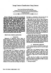
a solution, Sivic and Zisserman [11] demonstrated the feasibility of vector quantization, that is, clustering a sample of feature vectors into groups that can be thought of as “visual words.” Each feature vector in an image can be mapped to the closest of these cluster centers, thus creating a “bag of words” for that image. Sivic and Zisserman proceeded to apply standard text-retrieval methodology to retrieving frames in movies using TF-IDF scoring of word frequencies, cosine similarity between document vectors, and stop lists for very common or uncommon visual words. Nist´er and Stew´enius [12] took this visual-vocabulary scheme one step further. Unlike linguistic words, visual words are arbitrary cluster centers formed by quantizing a set of feature vectors. So instead of creating a single set of several thousand words, Nist´er and Stew´enius pointed out, one can just as well cluster in a hierarchical manner, creating a vocabulary tree. For instance, starting from the raw feature vectors, one can apply the k-means algorithm with, say, k = 10 to generate 10 children and then apply the process recursively on each of them. Continuing for six levels, the authors created 106 leaf nodes and 106 + 105 + . . . + 101 + 100 = 1, 111, 111 total words in the vocabulary. This was two orders of magnitude more than were used in [11], allowing for higher precision and recall of ground-truth movie frames. At the same time, the efficient tree indexing structure allowed for sub-second queries. The standard SIFT approach is to sample descriptors at keypoints identified through an interest-point detection algorithm [9]. For instance, Sivic and Zisserman [11] sampled at affine-covariant locations corresponding to “Shape Adapted” or “Maximally Stable” regions. However, Nowak et al. [7] noted that these locations are not chosen directly to optimize SIFT performance, so the assumption that interest points make good SIFT-descriptor points had not been verified. Nowak et al. compared Laplacian-of-Gaussian and Harris-Laplace keypoints against randomly chosen keypoints and found that the latter performed almost as well for small numbers of locations sampled. However, because there are only so many interest points in an image, the former methods tend to saturate at about 1,000 points per image, while the performance of random keypoints continues to increase with the number of points sampled. On account of this finding, Vedaldi [8] used random sampling of keypoints in his bag-of-visual-words image classifier. Figure 1, inspired partially by [13, p. 24], illustrates the bag-of-visual-words approach.

3.

FEATURE EXTRACTION

We base our feature-extraction and classification system on the open-source Matlab package called “Bag of features” developed by Vedaldi [8]. The program makes use of “SIFT++” [14], an open-source C++ implementation of Lowe’s SIFT feature-extraction method [9].

3.1

Keypoint Selection

We first choose 10,000 candidate keypoint locations at which to evaluate SIFT descriptors. Each location (x, y) is chosen uniformly at random throughout the image and is associated with a random scale σ. Larger scales correspond to more blurring, whereas smaller scales pick out more detailed local structure. Since nearby points with large scales will have similar descriptor values, we need fewer total largeσ points than small-σ points. In particular, we choose a

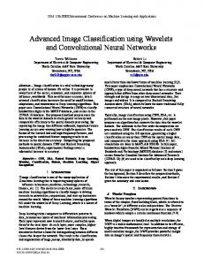
given σ with probability proportional2 to 1/σ over an interval [1, σmax ], σmax equal to one-tenth of the smaller of the width and height of the image. Figure 2a shows an example of random keypoints. While Nowak et al. [7, p. 496] found that the performance of interest-point detectors saturated at around 1,000 keypoints while random sampling showed continued performance improvements with more points sampled, the authors did not consider the possibility of combining the approaches: Starting with keypoints from an interest-point detector and then adding more random points. Though it was not our default approach, we experimented with this idea, using the output of Koo’s Canny edge detector [15] set to its default parameters. This typically gave 1,000-2,000 points, with the remaining 8,000-9,000 keypoints sampled randomly as before (see Figure 2b).

3.2

SIFT Descriptors

Once the keypoints are selected, we convert the input image to grayscale (PGM). This is processed by SIFT++ to give m 128-dimensional descriptor vectors for an image, where m ≤ 10, 000 is the number of accepted keypoints. We use the default parameter settings of SIFT++, with no rejection of points having small values for the Difference of Gaussian function. However, because many product images have quite a huge proportion of white space area–which are not informative for our classification task, we later reject keypoints whose SIFT descriptors have `2 norms smaller than a given threshold, experimentally chosen to be 50. This typically reduces the number of keypoints by 1,000-2,000 (see Figure 2c).

3.3

Constructing Visual Words

Given a collection of feature vectors for all training images, we construct a visual codebook using the method of Nist´er and Stew´enius [12]. This involves recursively applying the kmeans algorithm to the collection of feature vectors in order to generate a tree of visual words. If the number of data points in a group falls below k before we reach the leaf layer of the tree, we stop calling k-means and simply assign each of those points to its own cluster. There are a few questions to consider in constructing the vocabulary tree. • What fraction of the original data points should be included? Vedaldi’s original implementation retained a random 10% of the feature vectors to reduce computational time while clustering. We tried increasing this fraction to 100% and did find slight performance improvement; however, this considerably slowed the process of tree construction and required excessive amounts of RAM. We also experimented with reducing the fraction of feature vectors retained below 10%. In fact, using as few as 0.5% of the original feature vectors, we were able to maintain reasonable accuracy without incurring a large computational burden during cross-validation. We used 0.5% of the feature vectors for the results in this paper. (We do this only during tree construction; for evaluating frequency counts ` ´p 2 In fact, we tried probabilities proportional to σ1 for p between 0.5 and 2.0. Empirically, p between 1.0 and 1.25 gave roughly equally optimal performance, but we settled on p = 1.0 for simplicity.

of visual words in each image, as described in Section 3.4, we always use 100% of the feature vectors.)

Stew´enius [12, p. 6] found it to give better results than cosine similarity.

• In order to ensure “fairness” among the different categories, we include the same number of feature vectors from each category in the set of features that is clustered to form the codebook. For example, if a large class has twice as many images (and hence approximately twice as many feature vectors) as a small class, only about half as many feature vectors are taken from each image of the large class.

• d(s1 , s2 ) = 1 − cos(θ(s1 , s2 )), where cos(θ(s1 , s2 )) := s1 ·s2 . Cosine similarity is standard in information ks1 kks2 k retrieval and was used by Sivic and Zisserman [11, p. 4]. “ ” • d(s1 , s2 ) = 1 − exp − µ1 χ2 (s1 , s2 ) , where χ2 stands for chi-square distance, and µ is the average of all such distances over each pair of images. A chi-square-based kernel was proposed in [16] and used in [17, p. 4].

• What should be the branching factor of the tree, i.e., the k in k-means? Nist´er and Stew´enius [12, p. 10] used 10. We found performance improvements for larger values and settled on 100. • What should be the approximate number of leaves of the tree? After trying values between 250 and 20,000, we settled on 1,000, although using 5,00010,000 tended to give comparable performance. Incidentally, 1,000 leaves was found by Nowak et al. [7, p. 497] to be a rough optimum between having too few visual words on the one hand and overfitting on the other hand.

3.4

Image Signatures

In the tree of feature vectors computed as above, each node (including intermediate and leaf nodes) represents a visual word. Each image (“document”) has a set of m SIFT descriptors; each of these has its own path down the tree and, hence, its own set of words. The words corresponding to intermediate nodes in the tree have higher counts than those corresponding to leaves because more descriptors pass through them. For each image, we compute a signature s, that is, a vector of term frequency-inverse document frequency (TF-IDF) scores, exactly as in [11, p. 4]. The wth entry of the vector is « „ N , sw = nwi ln nw where nwi is the number of times word w appears in image i (the number of SIFT descriptors in i that pass through node w), nw is the number of images containing word w (the number of images with any SIFT descriptor passing through node w), and N is the number of images. We postprocess the signature vectors by cutting off values above a threshold and then normalizing.

4.

CLASSIFICATION

Classification proceeds by a nearest-neighbor algorithm applied to the signatures of each image. Below we describe the design details, including our choice of distance function, our use of a weighting scheme, and our method for combining information from multiple views of a product.

4.1

Distance Functions

We evaluated three functions for the distance d between a pair of signatures, s1 and s2 : P • d(s1 , s2 ) = j |s1 [j] − s2 [j]|, where si [j] is the jth component of the vector si . This is the `1 norm of the difference of the two signature vectors. Nist´er and

While the cosine and chi-square distances performed similarly, cosine was faster to compute, so we used it as the default.

4.2

Weighted Nearest Neighbor

A standard k-NN classifier assigns a test image t to that category with the plurality of votes among the k closest training images. One intuitive extension to this approach is to weight the votes of the training images by their closeness to the test image [18]. While theoretically less accurate on an infinite set of training examples [19], certain distanceweighted k-NN approaches have been found to perform better in practice [20]. We try a weighting scheme that we call “z-score voting.” Let k be a value between 1 and the total number of training images. For each image i among the k closest, image i votes for its own category label with a weight wi given by wi = −z-score(d(st , si )) =

µt − d(st , si ) , σt

where µt and σt are, respectively, the mean and standard deviations of all the distances from image t. Images that are closer to t will have more negative z-scores and hence larger numbers of votes; images that are far will actually get a negative number of votes. As an illustration, consider a two-class problem with training-image classes (1, 1, 2, 2). If the associated negative z-scores were (0.5, 0.5, −1.5, 0.5) and if k = 4, we would give class 1 a total of 0.5 + 0.5 = 1 vote and class 2 a total of −1.5 + 0.5 = −1 votes. Class 1 has more votes, so we predict that t belongs to class 1. We experimentally found best performance when we set k equal to the entire number of training images. In this case, the z-score procedure has an interesting interpretation: it chooses the class c that maximizes X X ´ ` µt − d(st , si ) wi = ∝ µt − d c N c , σt i : class(i)=c

i : class(i)=c

where Nc is the number of images in class c (excluding t) and dc is the average of the d(st , si ) values for c. Thus, the procedure rewards classes with small average distances, and the Nc factor gives more weight to classes with large numbers of labeled examples (helping them if dc < µt and hurting them otherwise).

4.3

Combining Views

A number of products on Amazon.com have multiple associated images, corresponding to views of the object from different orientations. We included all of the views of each product in our database of images, except in cases where the viewpoint available of the image is obviously unhelpful—e.g.,

Ballet shoes with legs

A pair of baseball shoes

Table 3: Examples of non-standard “viewpoints.”

a picture of the underside of a shoe when we were trying to discriminate shoes with lace from velcro, or the back of a high-heeled shoe when we wanted to determine whether the toe was pointy or not. Given this database, one approach is to ignore multiple views entirely, pretending that each image corresponds to a different product.3 However, this fails to take into account information from other viewpoints available and may even lead to inconsistent decisions if one view is assigned to a different category than another view of the same product. One way to combine the information from each view might be the following: Classify each view on its own, pretending that we have only one view of the product available; then, each of those decisions counts as a vote, and we choose the product’s category to be of the one with the most votes. However, this approach fails to consider the fact that some views may be more informative than others because it gives equal weight to every view. To fix this, one might assign weights to the votes of each view in inverse proportion to their distances to their near neighbors. Even after weighting the votes, there remains another problem: If we compare by analogy the different views of an image to different states in the USA, then it’s possible that one category could win the majority of votes among views (“win the electoral vote”), but—on account of “close elections” in those views—still be farther away from its category label than another category would have been when we average over the distances of all views to all training images (“losing the popular vote”). As a result, we take a slightly different approach. We calculate the distance from each view of a given product to all views of other products and concatenate those distances into one long list of distances to which z-score voting can be applied as usual. More informative views will have generally higher z-scores and so will automatically get more say in the final decision.

5. 5.1

EXPERIMENTAL SETUP Data Collection

We downloaded approximately 3,500 product images from the shoe and men’s shirt departments of Amazon.com and 3 Care must be taken to exclude all other images of the same item from the set of neighbor images. Otherwise, we could very well find that, say, the nearest neighbor to a velcro shoe viewed from the left is an image of the very same shoe viewed from the right. Treating the shoe viewed from the right as a neighbor whose label is known would be cheating.

other online stores, manually labeling them with tags for category, viewpoint, and product number. Table 1 shows the categories among which we wanted to distinguish; vertical lines separate the groups within which we wanted to classify images. For instance, we tried classifying “velcro vs. laced” sneakers, “pointy vs. nonpointy” high-heeled shoes, etc. The only one of these classification problem for which Amazon.com already provides separate tags is “ballet vs. boating vs. baseball”. Amazon.com provides multiple images for most of its shoes; examples of various views are shown Table 2. Some of the views were non-standard as Table 3 shows, but we included a few of them in our data sets to make the tasks more realistic.4

5.2

Evaluation

We test our classifier using 5-fold cross-validation; on each fold, we build our vocabulary tree from the first 4/5 of the images and classify on the remaining 1/5. Each image is assigned to the category of its near neighbors among the training images.5 The natural performance metric in this context is classification accuracy. While we could evaluate overall accuracy, doing so gives more weight to classes with smaller total number of images. For this reason, we instead follow Nowak et al. [7, p. 494] in reporting class-size-adjusted accuracies: i.e., a simple average of within-class accuracy over each class. For example, if our classifier predicted 10 out of 100 boating shoes and 5 out of 10 ballet shoes, the overall accuracy 10+5 = 13.6%, while the class-size-adjusted acwould be 100+10 ` 10 ´ 5 + 10 = 30%. curacy would be 21 100

6.

RESULTS AND DISCUSSION

In tables in this section, we report class-size-adjusted accuracies averaged over the five classification tasks in Table 1. (This is despite the fact that some of our problems have a baseline accuracy of 50% and others, 33%.) We combine the standard errors from 5-fold crossvalidation among the in five problems in quadrature as v u 5 X 1u overall SE = t (SE for problem i)2 . 5 i=1 In figures, we report separate standard errors for each problem, but averaged in quadrature over all the parameter settings.

6.1

Number of Keypoints

Various figures in Nowak et al. [7, p. 495] show that accuracy tends to peak at around 10,000 keypoints, which is the default number that we used. Table 4 confirms this finding, showing that varying the number of keypoints in either direction does not make a large difference. 4

If interested in using this data set, please see http://www.sccs.swarthmore.edu/users/09/btomasi1/ tagging-products.html 5 In theory, it would be permissible to use both training and testing images to build the vocabulary tree and then classify in a leave-one-out fashion without cross-validation; this is because construction of the vocabulary tree is unsupervised. However, such an approach requires having all testing images available when the classifier is built, which is unrealistic in many applied settings.

Category

Velcro

Laces

Pointy

Nonpointy

Short Sleeve

Long Sleeve

Sample image Num. products Num. individual images Avg. views per product

75 299 ∼4

75 390 ∼5

77 414 ∼5

63 360 ∼6

150 152 ∼1

147 152 ∼1

Category

Ballet

Boating

Baseball

Collar

V-Neck

Crew

Sample image Num. products Num. individual images Avg. views per product

50 53 ∼1

98 453 ∼5

66 205 ∼3

100 100 ∼1

97 99 ∼1

100 105 ∼1

Table 1: The product categories we collected. Our goal was to distinguish individual categories from among those categories grouped by the vertical lines.

Back

Front

Top Left

Top Right

Bottom Left

Bottom Right

Left-Angled

Right-Angled

Left Lateral

Right Lateral

Table 2: Different viewpoints available for shoes. Not all were available for all products. Moreover, not all of those available were used; for instance, we didn’t include “back” views for the pointy-nonpointy classification even though they were available.

Num. keypoints

Accuracy ± SE (%)

5,000 10,000 15,000

81.5 ± 0.9 81.9 ± 0.9 81.8 ± 0.8

Table 4: Class-size adjusted accuracies as we increase the number of keypoints.

6.2

Number of Training Examples

Our basic z-score-voting procedure uses the distances to all other images, but we could modify it to use only a certain fraction of the closest neighboring images, as with regular kNN. This idea sounds like it might be particularly helpful for those categories (in our case, the shoes) that have multiple views, because we might imagine that very different views of a shoe will have large distances regardless of category and, hence, will contribute little information. However, we found that doing this degraded performance, even for multipleview classification tasks.

6.4

Keypoint Detector Keypoint detector

Avg. acc. ± Avg. SE (%)

Only Canny (∼2,000 keypoints) Only random (∼2,000 keypoints) ∼2,000 Canny, ∼8,000 random ∼10,000 random

82.9 ± 0.9 83.1 ± 1.1 83.8 ± 0.9 81.4 ± 0.7

Table 6: Performance for various choices of keypointdetection method. Table 6 reports the results of using a Canny edge detector combined with random selection of keypoints rather than entirely random keypoints. While the Canny+random approach appears to do well, the variations from task to task are too large to draw firm conclusions, as is evident from the fact that classification with 10,000 random keypoints happened to do worse on average than with only 2,000.

6.5

Multiple Views

Figure 3: Class-size-adjusted accuracies improved as we increased the number of products in our training set. Figure 3 shows how performance improves with increasing numbers of product training examples from each category. We constructed it by artificially reducing the size of our labeled data to random subsets. The problems clearly differ in their difficulty, with some being relatively easy; for instance, we can distinguish short-sleeve vs. long-sleeve shirts to 90% accuracy with only 5 training images.

6.3

z-Score Voting Classification method

Avg. acc. ± Avg. SE (%)

k-NN, k = 5% all products k-NN, k = 10% all products k-NN, k = 20% all products z-score voting, all products

76.8 ± 1.2 71.7 ± 1.3 61.4 ± 1.3 81.6 ± 0.8

Table 5: The z-score voting procedure outperforms standard k-NN for k = 5%, 10%, and 20% of the images. Table 5 shows the performance of a k-NN classifier with k set to 5%, 10%, and 20% of the total number of product images. However, the z-score voting procedure—which takes into account not just whether each training image is a “near neighbor” but how far it is from the test image—results in significantly higher performance.

Figure 4: Accuracy improved as we increased the number of views used for each product. Figure 4 shows the improvement in performance that results from using more and more views of each product, where information from the views is combined as described in Section 4.3. We chose random subsets of the views to artificially reduce the number of views available.

7.

FUTURE DIRECTIONS

We achieved accuracies between 66% and 98% on 2- and 3class classification problems, showing that at least for some tasks, tagging products based solely on their images can be done in an automated fashion. Even though we optimized the parameters of our classifier, its basic structure was relatively simple. Recent work in image classification has begun moving “Beyond bags of features”—as one paper put it [21]—toward methods that preserve information about the locations of features within an image. One simple and popular way to do this is “spatial pyramids,” i.e., dividing an image into sub-rectangles and computing histograms over each of those regions separately in addition to over the entire image [21]. Bosch et al. [17] have recently demonstrated state-of-the-art performance on the Caltech 101 and 256 data sets, including 96.6% accuracy on Caltech 101 (p. 22), using a spatial-pyramid approach with histograms of both visual words computed from SIFT descriptors as well as oriented gradient vectors. It would be interesting to see whether this extension would improve product-image classification. Utilizing information about spatial locations in an image could be particularly helpful in our case because, unlike natural images, product images (at least from the same view) have relatively constant locations for salient points, e.g., the toe of a woman’s high-heeled shoe. Finally, we should note that despite our system’s good performance on some tasks, commercial application of our image classifier could be harder due to our lack of control over image dataset. For instance, when we searched for “sneakers” on Amazon.com in order to find examples of some with laces and some with velcro, we also found a number of products that didn’t fall neatly into either category, such as shoes with no straps at all, and “sneaker balls” for odor removal. We didn’t include such images in our data set, but a real-world classifier would have to deal with them.

Acknowledgments We thank Lorrin Nelson and Wally Tseng at Amazon.com for suggesting this topic and providing guidance about how an image classifier might be used commercially. We also thank A. Vedaldi for making available the original “Bag of features” code, as well as our classmates in the Swarthmore College Fall 2008 Senior Conference for providing feedback on our manuscript.

8.

REFERENCES

[1] M. Everingham, A. Zisserman, C. K. I. Williams, L. Van Gool, M. Allan, C. M. Bishop, O. Chapelle, N. Dalal, T. Deselaers, G. Dorko, et al. The 2005 PASCAL Visual Object Classes Challenge. Lecture Notes in Computer Science, 3944:117, 2006. [2] M. Everingham, L. Van Gool, CKI Williams, J. Winn, and A. Zisserman. The PASCAL Visual Object Classes Challenge 2007 (VOC2007) Results, 2007. [3] Li Fei-Fei, R. Fergus, and P. Perona. Learning generative visual models from few training examples: An incremental bayesian approach tested on 101 object categories. page 178, 2004. [4] G. Griffin, A. Holub, and P. Perona. The caltech-256. Technical report, Caltech, 2007.

[5] Jutta Willamowski, Damian Arregui, Gabriella Csurka, Christopher R. Dance, and Lixin Fan. Categorizing nine visual classes using local appearance descriptors. In In ICPR Workshop on Learning for Adaptable Visual Systems, 2004. [6] Jianguo Zhang, Marcin Marszalek, Svetlana Lazebnik, and Cordelia Schmid. Local features and kernels for classification of texture and object categories: A comprehensive study. In CVPRW ’06: Proceedings of the 2006 Conference on Computer Vision and Pattern Recognition Workshop, Washington, DC, USA, 2006. IEEE Computer Society. [7] Eric Nowak, Fr´ed´eric Jurie, and Bill Triggs. Sampling strategies for bag-of-features image classification. pages 490–503. 2006. [8] A. Vedaldi. Bag of features. http://www.vlfeat.org/∼vedaldi/code/bag/bag.html. [9] D. Lowe. Distinctive image features from scale-invariant keypoints. IJCV ’04, 60(2):91–110. [10] O. Boiman, I. Rehovot, E. Shechtman, and M. Irani. In Defense of Nearest-Neighbor Based Image Classification. In Computer Vision and Pattern Recognition, 2008. CVPR 2008. IEEE Conference on, pages 1–8, 2008. [11] J. Sivic and A. Zisserman. Video google: A text retrieval approach to object matching in videos. In ICCV ’03. [12] D. Nist´er and H. Stew´enius. Scalable recognition with a vocabulary tree. In CVPR ’06, pages 2161–2168. [13] A. Bosch. Image classification for a large number of object categories. PhD thesis, Departament d’Electr` onica, Inform` atica i Autom` atica, Universitat de Girona, 2007. [14] A. Vedaldi. Sift++: A lightweight c++ implementation of sift. http://www.vlfeat.org/∼vedaldi/code/siftpp.html. [15] John Koo. Canny edge detector algorithm and matlab codes. http://black.csl.uiuc.edu/∼yima/imgproc/cacode.html. [16] A. Bosch, A. Zisserman, and X. Munoz. Representing shape with a spatial pyramid kernel. In Proceedings of the 6th ACM international conference on Image and video retrieval, pages 401–408. ACM Press New York, NY, USA, 2007. [17] A. Bosch, A. Zisserman, and X. Munoz. Image classification using rois and multiple kernel learning. IJCV ’08. [18] S. Dudani. The distance-weighted k-nn rule,”. IEEE Trans. Syst, Man Cybern, 6(4):325–327, 1976. [19] T. Bailey and AK Jain. A note on distance-weighted k-nearest neighbor rules. IEEE Transactions on Systems, Man, and Cybernetics, 8(4):311–313, 1978. [20] JES Macleod, A. Luk, and DM Titterington. A Re-Examination of the Distance-Weighted k-Nearest Neighbor Classification Rule. Systems, Man and Cybernetics, IEEE Transactions on, 17(4):689–696, 1987. [21] S. Lazebnik, C. Schmid, and J. Ponce. Beyond bags of features: Spatial pyramid matching for recognizing natural scene categories. In CVPR ’06, volume 2.

Figure 1: Illustration of the bag of visual words approach that we use for classification. The first row shows the process of learning a vocabulary of visual words by (i) selecting keypoints from each image, (ii) - (iii) computing SIFT descriptor vectors at those keypoints, and (iv) clustering the entire collection of SIFT descriptors into groups whose centers will define the visual words. We cluster into k groups (k = 3 shown, k = 100 used) and then recursively cluster each of those groups to create a tree of cluster centers. The second row shows how we use the visual-word tree. (v) Given an image, we (vi) again compute SIFT descriptors at keypoints and then (vii) walk each descriptor down the vocabulary tree using the closest cluster centers. Each time a descriptor walks through a cluster center, we increment the frequency count for that visual word. (viii) The result is a histogram of visual-word counts.

(a) Random

(b) Random plus Canny

(c) Small-SIFT points removed

Figure 2: Illustrations of chosen keypoints by red circles, whose radius is equal to the scale σ. To avoid clutter, these figures 1 show only keypoints with σ ≤ 10 pixels; however, the maximum possible σ is actually 10 min {280, 280} = 28 pixels for this 280 x 280 image. Panel 2a shows roughly 5,000 random keypoints. 2b shows random keypoints plus points found by the Canny edge detector, such that the total number of keypoints is the same as in 2a. 2c is the same as 2b except that points are removed that have SIFT descriptors with `2 norm less than 50. This removes about 1,000 keypoints in pure white space. Some points remain on white space in the figure because their descriptor values are influenced by pixels that lie outside of the one-σ radius shown.