arXiv:nlin/0106022v1 [nlin.CD] 15 Jun 2001. Taming chaos by impurities in two-dimensional oscillator arrays. M. Weiss, Tsampikos Kottos, and T. Geisel.
Taming chaos by impurities in two-dimensional oscillator arrays
arXiv:nlin/0106022v1 [nlin.CD] 15 Jun 2001
M. Weiss, Tsampikos Kottos, and T. Geisel Max-Planck-Institut f¨ ur Str¨ omungsforschung, and Institut f¨ ur Nichtlineare Dynamik der Universit¨at G¨ottingen, Bunsenstraße 10, D-37073 G¨ottingen, Germany The effect of impurities in a two-dimensional lattice of coupled nonlinear chaotic oscillators and their ability to control the dynamical behavior of the system are studied. We show that a single impurity can produce synchronized spatio-temporal patterns, even though all oscillators and the impurity are chaotic when uncoupled. When a small number of impurities is arranged in a way, that the lattice is divided into two disjoint parts, synchronization is enforced even for small coupling. The synchronization is not affected as the size of the lattice increases, although the impurity concentration tends to zero.
In order to observe spatio-temporal patterns for smaller couplings, the geometrical arrangement of the impurities is shown to play a crucial role. Specifically we show that an impurity configuration that divides the lattice into at least two disjoint parts is most appropriate for the creation of synchronized solutions. Such configurations will always produce patterns that locally can be identified as lines, provided the coupling is above a threshold value. The resulting spatio-temporal patterns are stable with respect to an increase of the system size, indicating that an impurity concentration that tends to zero may suffice to lead to synchronization.
I. INTRODUCTION
Coupled arrays of oscillators are studied extensively in many fields of science because of their prevalence in nature. They are used as models for coupled arrays of neurons [1], chemical reactions [2], coupled lasers [3] or Josephson junctions [4], charge-density-wave conductors [5], crystal dislocations in metals [6], and proton conductivity in hydrogen-bonded chains [7]. Various models and coupling schemes have been proposed and analyzed previously [8]. A particular class are arrays of coupled oscillators, which exhibit chaotic motion when uncoupled. This class includes the forced Frenkel-Kontorova model [9], which finds a straightforward physical realization in an array of diffusively coupled Josephson junctions [10,11], in which the applied current of each junction is modulated by a common frequency. The possibility to obtain synchronized motion in such systems has been investigated recently by Braiman et al. for the case of one- (1D) and two-dimensional (2D) chaotic arrays of forced damped nonlinear pendula [12] and coupled Josephson junctions [13]. They observed the emergence of complex but frequency-locked spatio-temporal patterns, in which the chaotic behavior was completely suppressed, when a certain amount of disorder had been introduced by randomizing the lengths of the pendula. In Ref. [14] the same phenomenon has been investigated from a completely different point of view: It was shown for 1D arrays of coupled chaotic pendula, that introducing a single impurity at a particular site is sufficient to lead to complete synchronization. In this paper we study 2D arrays of coupled chaotic pendula. We ask for the minimal coupling as well as the influence of concentration and arrangement of impurities, needed to observe spatio-temporal patterns. Although for geometrical reasons one might expect that a single impurity cannot play the role it plays in 1D arrays, we find that it is able to tame the chaotic behavior of an arbitrarily large 2D array, provided that the coupling is strong enough. A single impurity can produce synchronized spatio-temporal patterns, even though all oscillators and the impurity are chaotic when uncoupled.
II. MODEL
We will focus our analysis on the model examined in Refs. [12,14]: 2 θ¨n,m + γ θ˙n,m = −gln,m sin θn,m + τ ′ + τ sin ωt ln,m +k(θn+1,m + θn−1,m − 4θn,m + θn,m+1 + θn,m−1 ), (1)
where n, m = 1, 2...N . Thus, there is a damped, driven pendulum with unity mass and length lnm on each site (n, m) of the lattice, subject to an ac and a dc torque. The parameters used are the gravitational acceleration g = 1, the dc torque τ ′ = 0.7155, the ac torque τ = 0.4, the angular frequency ω = 0.25, and the damping γ = 0.75. Neighbouring pendula are coupled via a discrete Laplacian, where k denotes the coupling strength. We have chosen free boundary conditions, i.e. θ0,m = θ1,m , θN,m = θN +1,m , θn,0 = θn,1 , θn,N = θn,N +1 and used a fourth order Runge-Kutta routine with a time step dt = 0.01 to numerically integrate Eq. (1). We carefully checked that decreasing the time step to dt = 0.001 did not alter our results. A very convenient measure that allows a quick visualization of the average global spatio-temporal behavior of the lattice, is the average velocity σ(jT ) =
1
N ·M X 1 θ˙n (jT ) N · M n=1
(2)
at multiple times of the driving period T = 1/ω. Using this quantity [15] to obtain a bifurcation diagram not only can ascertain if chaotic or periodic behavior is obtained, but in addition helps to identify the maximum period of a pattern: Computing σ(t) at each period t = jT of the driving, will lead to a periodic sequence σ1 , ..., σp , σ1 , ..., when transients have died out and a spatio-temporal pattern of periodicity p (’Pp attractor’) has emerged. In practice we inspect the last 20 values of σ(jT ) with j = 1, ...170, so that transients have died out. Thus, P20 attractors or attractors of larger periodicity are not recognized as such but rather appear as chaotic attractors. Applying this strategy to an isolated pendulum, a bifurcation analysis with respect to the pendulum length l was performed in Ref. [14]. This approach revealed that each isolated pendulum is chaotic for values l = 1 ± 0.002 and that three more chaotic windows exist: Two narrow ones at l ≈ 0.84, and l ≈ 0.52, and a broad one for l < 0.35. Thus we know whether a chosen pendulum with length l is chaotic or not. Furthermore, for the above chosen parameter values it is known, that pendula with ln,m > 1 and ln,m < 1 show libration and rotation, respectively, apart from the windows, where chaotic motion appears.
1.0
σ
(a)
(b)
(c)
(d)
0.5
0.0 1.0
σ
0.5
0.0
0
0.2 0.4 0.6
0.8
limp1
0
0.2 0.4 0.6
0.8
limp1
FIG. 1. Bifurcation diagram for a 50 × 50 lattice of coupled pendula with length ln,m = 1. A single impurity with length limp is located at lattice site (25,25). For each limp the values of σ(151T ), ..., σ(170T ) are shown, where T is the period of the driving. The coupling is (a) k = 1, (b) k = 2, (c) k = 3, and (d) k = 5. In (c) the first windows of synchronization can be observed, which enlarge for bigger couplings (d).
In order to illustrate the occurence of this P4 pattern in a better way, we show in Fig. 2 a typical gray scale plot of the velocities θ˙n,m as a function of the lattice coordinates (n, m). The stroboscopic snapshots are taken with a time lag of one period of the driving T ; darker shading indicates higher velocity. In this example we used 64 × 64 oscillators having ln,m = 1 and located an impurity of length limp = 0.1 in the middle of the lattice at (32, 32). The coupling constant is k = 5. After some transient (not shown) the synchronization is maintained and a P4 attractor is clearly visible. We neglect edge effects except to remark that they are strictly confined to the last few pendula near the boundaries. Moreover, they become very regular if the calculation is carried on for longer times.
III. RESULTS AND DISCUSSION
The simplest configuration of a 2D lattice described by Eq. (1), is that of a single impurity in a sea of identical chaotic pendula with length ln,m = 1. We fixed the lattice size to be 50 × 50, with the the impurity located at site (25, 25) and made a bifurcation analysis with respect to the impurity length limp for various values k of the coupling. In Fig. 1 the obtained bifurcation diagrams for k = 1, 2, 3, 5 are plotted versus limp . For convenience we normalized σ to take on values in the unit interval [0, 1]. Similarly to 1D arrays we find, that one impurity is able to organize the 2D arrays. However, our bifurcation analysis shows that the coupling constant has to be larger than kcr ≃ 3, whereas in the 1D case k ≥ 0.1 was sufficient [14] to produce spatio-temporal patterns. We would like to point out the appearance of a P4 attractor for k = 5, limp < 0.15 in Fig. 1d. Here an array of chaotic pendula is synchronized by a single impurity, which itself is chaotic, when isolated.
t=180T
t=181T
t=182T
t=183T
t=184T
t=185T
t=186T
t=187T
FIG. 2. Snapshots of θ˙n,m for a 64 × 64 lattice with ln,m = 1, limp = l32,32 = 0.1 and k = 5 at multiple times of the driving period T .
In many applications, however, one is interested in the weak coupling limit [16]. In this limit, our analysis shows 2
It is thus natural to ask wether a line of impurities is the only geometry that can produce spatio-temporal patterns for relatively small values of the coupling constant. In Fig. 3b,c we report the P1 attractors of a lattice of 128 × 128 coupled pendula with lengths ln,m = 1, limp = 0.7 and coupling k = 0.5, where the impurities are arranged like a cross (Fig. 3b) or as a ring (Fig. 3c). In both cases the observed pattern geometries consist locally of stripes as was also observed for the ’line-geometry’ in Fig. 3a. What is the common geometrical feature of the above impurity configurations that allow them to control the chaotic lattice? From the above analysis we draw the conclusion, that it is sufficient for synchronization, that the impurites divide the lattice into at least two disjoint subregions. In that way the critical coupling needed to observe a spatio-temporal pattern is decreased by an order of magnitude. Reducing the coupling below kcr ≈ 0.1, however, suppresses the formation of spatio-temporal patterns even for these lattices. This finding is consistent with earlier investigations on 1D arrays, which revealed a critical coupling k ≈ 0.1, below which no pattern formation could be observed. Furthermore, the observed P1 pattern for the ’line geometry’ (Fig. 3a) is analogous to the 1D case, where the introduction of a single impurity caused the same topology of the array, i.e. a division into two disoint sets, and a similar pattern was observed [14]. Thus, the results of the 1D case define the limiting kvalue also for the 2D lattice.
that one impurity is not able to create spatio-temporal organization of a chaotic lattice. Therefore, it is meaningful to ask whether spatio-temporal patterns can emerge at all and under which conditions they may be obtained. To this end we increase the number of impurities introduced in the lattice and investigate the importance of their geometrical arrangement as well as their concentration. In Fig. 3a we report the P1 pattern emerging for a 128 × 128 lattice with coupling constant k = 0.5, when 128 impurities were arranged along a line in the middle of the lattice, dividing it into two disjoint parts. The same behavior could be observed even for smaller couplings. We verified this for coupling constants as small as kcr = 0.1. Moreover, we found that increasing the size of the lattice to N = 256 (the limit of our computational capability), but maintaining the line-like geometry of impurities and the parameter-values, did not affect the formation of a pattern. In all cases we observed synchronization to a P1 pattern after an initial transient. Thus, increasing the size of the lattice will not affect the pattern formation although the percentage of the impurities will tend to zero in the limit of infinite systems. This indicates that the concentration of impurities is not of primary importance. To test the influence of the special arrangement of impurities, we considered a 128 × 128 lattice with k = 0.5 and 128 impurities of length limp = 0.7 located at random positions of the lattice. In all cases we have studied we obtained chaotic patterns. Even an increase of their concentration by more than a factor of 3 did not produce any spatio-temporal pattern. (a)
(b)
(a)
0.5
0.5
σ
0.0 0 20 40 60 80
0.0 0 20 40 60 80
20
40
60
80
j
0.0 0
20
40
60
80
j
(c) t=150T
t=151T
t=152T
t=153T
t=154T
t=155T
t=156T
t=157T
t=158T
t=159T
t=160T
t=161T
0.5
σ
j
0.5
σ
(c)
0.0 0
0.5
(b)
σ
σ
j
0.0 0 20 40 60 80
FIG. 4. (a) Chaotic sequence σ(jT ) for a 128 × 128 lattice (k = 0.5) with ln,m ∈ [0.998, 1.002]. (b) Periodic sequence σ(jT ) for a 128 × 128 lattice (k = 0.5) with ln,m ∈ [0.8, 1.2]\[0.998, 1.002] revealing a P6 pattern. (c) Snapshots at multiple periods T of the driving confirm the existence of a P6 pattern as predicted in (b).
j
FIG. 3. Snapshots of θ˙n,m for a 128 × 128 lattice with ln,m = 1, limp = 0.7 and k = 0.5. The impurities are positioned as indicated in the upper panel: (a) on a line along n = 64, (b) on a cross along the lines n = 64 and m = 64, (c) on a square with (n, m) = (63, 63) the lower left and (66, 66) the upper right corner. In the lower panel, the corresponding σ(jT ) is shown.
We finally examined the effect of disorder and the possibility of obtaining self-organization or frequency locking. For a 128 × 128 lattice we randomly varied the 3
lengths of the pendula but restricted the range of the disorder such, that each individual pendulum is chaotic, i.e. ln,m ∈ [0.998, 1.002]. We found that the emerging pattern was always chaotic for a large number of different realizations of disorder and initial conditions. The lacking synchronization can be observed in a better way by inspecting σ(jT ), which does not show any periodicity (see Fig. 4a for an example). If the range of disorder is increased to include also regular moving pendula, i.e. ln,m ∈ [0.8, 1.2], self organization is possible in agreement with findings of Ref. [12]. This can be understood by the observation that synchronization already occurs, when choosing the disorder from an interval of pendulum lengths associated with regular motion, i.e. ln,m ∈ [0.8, 1.2]\[0.998, 1.002]. A particular example for this is shown in Figs. 4b,c, where the occurence of a P6 pattern can be observed. Thus, taking the lengths from the entire interval ln,m ∈ [0.8, 1.2] on average yields only 1% chaotic pendula, whose motion will be overdominated by the synchronizing regular ones, explaining the spatio-temporal pattern observed in Ref. [12].
[3] G. Kozyreff, A G. Vladimirov, and P. Mandel, Phys. Rev. Lett. 85, 3809 (2000); H.G. Winful and L. Rahman, Phys. Rev. Lett. 65, 1575 (1990); J. Terry, K.S. Thornburg, A.D.J. DeShazer, G.D. VanWiggeren, S. Zhu, and P. Ashwin, Phys. Rev. E 59, 4036 (1999); A. Hohl, A. Gavrielides, T. Erneux, V. Kovanis, Phys. Rev. Lett. 78, 4745 (1997). [4] A.V. Ustinov, M. Cirillo, and B. Malomed, Phys. Rev. B 47, 8357 (1993); K. Wiesenfeld, P. Colet, and S. Strongatz, Phys. Rev. Lett. 76, 404 (1996). [5] S.H. Strogatz-SH, C.M. Marcus, R.M. Westervelt, R.E. Mirollo, Physica D 36, 23 (1989). [6] E.N. Economou, Green’s Functions in Quantum Physics, Springer Series in Solid State Physics, Vol. 7 SpringerVerlag, Berlin, (1979). [7] A.V. Ustonov, B.A. Malomed, and S. Sakai, Phys. Rev. B 57, 11691 (1998); O.M. Braun and Yu.S. Kivshar, Phys. Rep. 306, 1 (1998); E. Nylund, K. Lindenberg, G. Tsironis, J. Stat. Phys. 70, 163 (1993). [8] J.F. Heagy, L.M. Pecora, and T.L. Carrol, Phys. Rev. Lett. 21, 4185 (1995); J.F. Heagy, T.L. Carrol, and L.M. Pecora, Phys. Rev. E 50, 1874 (1994). [9] L.M. Floria and J.J. Mazo, Adv. in Phys. 45, 505 (1996). [10] A.V. Ustinov, M. Cirillo and B.A. Malomed, Phys. Rev. B 47, 8357 (1993). [11] S. Pagano, M.P. Soerensen, R.D. Parmentier, P.L. Christiansen, O. Skovgaard, J. Mygind, N.F. Pedersen, and M.R. Samuelsen, Phys. Rev. B 33, 174 (1986). [12] Y. Braiman, J.F. Lindner, and W.L. Ditto, Nature 378, 465 (1995). [13] Y. Braiman, W.L. Ditto, K. Wiesenfeld, and M.L. Spano, Phys. Lett. A 206, 54 (1995). [14] A. Gavrielides, Tsampikos Kottos, V. Kovanis, and G.P Tsironis, Phys. Rev. E 58, 5529 (1998); Europhys. Lett. 44, 559 (1998). [15] There is a variety of related quantities, that may be defined in a similar way. However, we use σ(jT ) as a particular intuitive measure, that furthermore is easy to calculate. [16] H.G. Winful and L. Rahman, Phys. Rev. Lett. 65, 1575 (1990).
IV. CONCLUSION
In conclusion we have demonstrated that a lattice of chaotic pendula can be frequency locked into a spatiotemporal pattern by introducing impurities in the lattice. In the strong coupling limit, a single impurity can tame chaos. Decreasing the coupling constant requires more impurities in order to observe self-organization. In this case the geometry of the impurity configuration plays an important role. Our results suggest that if the impurity configuration divides the lattice into at least two disjoint parts then the coupling constant may be decreased without affecting the synchronization of the chaotic array. Moreover, the induced spatio-temporal patterns are then unaffected by the size of the lattice. Below the critical coupling kcr ≈ 0.1 no synchronization is observed. The value of this critical coupling is dictated by the minimum coupling which leads to the formation of spatio-temporal patterns in the 1D case. We are grateful to T. Gavrielides, V. Kovanis, A. Politi, and G Tsironis for helpful discussions.
[1] D. Amid, Modelling Brain Function, Cambridge University Press, Cambridge, UK 1989; J. Hertz, A. Krogh, R. Palmer, Introduction to the theory of Neural Computation, Addison-Wesley, Redwood City (1991). [2] A. Arneodo, J. Elezgaray, J. Pearson, T. Russo, Physica D 49 141, (1991); G.K. Schenter, R.P. McRae, B.C. Garrett, J.Chem. Phys. 97, 9116 (1992).
4