Absrract - The finite element solution of the vector wave equation often results in non-physical behavior known as spurious modes. It is shown that the ...
IEEE TRANSACTIONS ON MAGNETICS, VOL. 27, NO. 5 , SEPTEMBER 1991
4032
TANGENTIAL VECTOR FINITE ELEMENTS FOR ELECTROMAGNETIC FIELD COMPUTATION J. F. Lee Electromagnetic Communication Lab. 1406 W Green St. Department of Electrical and Computer Engineering University of Illinois at Urbana-Champaign Urbana, IL 61801
D. K. Sun and Z. J. Cendes Ansoft Corporation Four Station Square Pittsburgh, PA 15219
Absrract - The finite element solution of the vector wave equation often results in non-physical behavior known as spurious modes. It is shown that the occurrence of spurious modes is due to the improper modeling of the nullspace of the curl operator. One approach t o eliminating spurious modes is the use of tangential vector finite elements. With tangential vector finite elements, only the tangential components of the vector field a r e made continuous across the element boundaries. The use of this type of element has the following advantages: (1) The physical continuity requirements of the electric and magnetic fields a r e satisfied; (2) The interfacial boundary conditions are automatically obtained through the natural boundary conditions built into the variational principle; and (3) Dirichlet boundary conditions a r e easily set along curved boundaries. Edge-elements a r e the simplest example of tangential vector finite elements. However, edge-elements provide only t h e lowest-order of accuracy in numerical computations since in this approach the tangential component of the field is assumed to be constant along each edge of the element. I n this paper, t h e configurations of the tangential vector finite elements which a r e of higher-order approximations on twodimensional triangular elements as well a s on threedimensional tetrahedral elements a r e presented. The vector-valued basis functions a r e written explicitly, and the interpolatory meanings of the unknowns a r e also derived.
is of higher-order approximation in two- and three-dimensions. This family of TVFEM is complete to the fist-order in the range of the curl operator. Therefore, we denote this type of TVFEM as Hl(cur1) elements. Our contributions are: (1) The extension of the work of Kotiuga [4] to derive the estimation of the number of unknowns based upon the mesh information; (2) The presentation of the unknowns of the Hl(cur1) elements in two-dimensional triangular elements and three-dimensional tetrahedral elements; (3) The derivation of the corresponding vector basis functions makes the evaluation of element matrices possible; and (4) The description of the interpolatory meanings of the scalar unknowns. In this way, the post processing of the finite element solution can be done in much the same way as in conventional nodal finite element approaches. The remainder of this paper is organized as follows: Topological identities which are the extensions of reference [4] are presented in section 11. The configuration and the vector basis functions of the Hi(cur1) elements in R2 and R3 are discussed in section 111 and section IV, respectively. In section V, numerical experiments are used to verify theorectical predictions of matrix size. Finally, the conclusion and brief discussions are given in section VI.
INTRODUCTION As early as 1979, Nedelec introduced (reference [ 11) some
families of finite elements in R3, one of which conforms in the function space H(cur1). This family of finite elements has a very important property. The tangential component of the vector unknown is continuous across the element boundaries; this is not necessarily true for the normal component. Therefore, in this paper, we refer to this type of vector finite element methods as tangential vector finite element methods (TVFEM). By using the TVFEM, the nullspace of the curl operator in the discretized form is modeled exactly, and therefore no spurious modes are generated. Unfortunately, in reference [l], Nedelec addressed neither the constructions of such elements nor the corresponding vector basis functions. Consequently, the application of these elements has been limited. Independently, Bossavit [2] proposed using the so-called edgeelements for electromagnetic computation in R3. The edge-elements are the 1-form of the Whitney elements [3] and also tum out to be the same as the lowest order of H(cur1) elements in reference [ 11. In the current study, we present one family of TVFEM which
TOPOLOGICAL IDENTITIES In the application of the finite element methods, it is useful to know the total number of unknowns from the discretization of the problem domain before generating the matrix equation. With this information, the computation time as well as the memory requirement of the current problem can be estimated. In this section, we present some topological relations and an observation which is based upon the Delaunay triangulation (tessellation) [5]. From these relations, in the later sections, we are able to determine the total number of unknowns of the Hl(cur1) elements from the discretization. Most of the framework of this section is based upon the work of Kotiuga [4].
Two-dimensionalCase For a given triangulation in R2, the geometric entities are related by the following equations [6]: V -E + F = x2 2E - B = 3F (1)
G318-9464/91$01.00 0 1991 IEEE
lEEE TRANSACTIONS ON MAGNETICS, VOL. 27, NO.5, SEPTEMBER 1991
4033
where V is the number of vertices, E is the number of edges, B is the number of edges on the boundary, and F is the number of triangles of the triangulation. Here x2 is the Euler characteristicsin R2.
the set of piecewise linear functions in the discretized problem domain R. We also define uT = uxax+uyay and Vz=axax + ayay. The two-dimensional Hl(cur1) element has been applied in reference
Three-dimensionalCase
[7] to analyze the dispersions of dielectric waveguides. Unknowns in the Hi (curl) element are assigned as shown in Fig. 2. The tangential projection of the vector field uT along edge ( i j ) is determined by two unknowns U{ and uf . In addition, two
J
facial unknowns fo and f l are added to provide a quadratic approximation of the normal component of the field along two of the three edges. Therefore, there are eight degrees of freedom in a triangular element to describe the transverse components of a vector Figure 1: An ideal Delaunay triangulation around a vertex
For a tessellation of a three-dimensional region R, the Euler formula [6]states that V -E + F - T = x3 where T is the number of tetrahedra of the tessellation in R3. Here,
x3 is the Euler characteristicsof the three-dimensional region R.
However, in three dimensions, except for the faces on the boundaries, each triangular face is shared by two tetrahedra. Furthermore, one tetrahedron is formed by four triangular faces, which results in 4T = 2F - D (3) where D is the total number of boundary faces. In practical applications, the discretization (or the finite element mesh) is usually generated by using the Delaunay tessellation [ 5 ] . In two-dimensions, the Delaunay triangulation is the mangulation which maximizes the sum of minimum angles of the mangles. In Fig. 1, we show an ideal Delaunay triangulation around a vertex point. From Fig. 1, we expect, on average, that one vertex point is shared by six edges. Based upon this observation, we make the following assumption: For a Delaunay tessellation in three dimensions, a vertex point, on average, is shared by 6312 edges. Since one edge is formed by two vertices, we obtain 2E = G3I2V. (4) From equations (2), (3) and (4), we are able to determine the number of edges E from T and D, i.e. E = 1.16T + 0.579D (5) Notice that equation ( 5 ) is an approximation and holds true asymptotically. The expression on the right-hand-side of equation (5) should be rounded to the nearest integer to give the estimated E.
field. Note that in Fig. 2, the edge variables
4
and ui are common
J
unknowns across element boundaries. Thus, the tangential continuity of the field uT is assured. However, the facial variables fo. f l are local unknowns associated with each triangular element. These two facial variables are included to provide a complete linear approximation for V,xuz. 0
0
U2 1
2
U1
U:
Figure 2 Two-dimensionalHl(cur1) tangential finite element
The two vector basis functions of edge ( i j ) are