summarizes the famous Whitney elements, both 1-forms and 2-forms; the extension of the Whitney. (edge) elements to higher-order vector nite elements which ...
TANGENTIAL VECTOR FINITE ELEMENTS AND THEIR APPLICATION TO SOLVING ELECTROMAGNETIC SCATTERING PROBLEMS Jin-Fa Lee ECE Dept., WPI Worcester, MA 01609
1 INTRODUCTION The problem of computing electromagnetic wave scattering, either in a semi-closed domain like a waveguide discontinuity, or in an open domain such as RCS calculations, has been a topic of much theoretical and practical importance. To address this issue, Finite Element Methods (FEMs) have been applied extensively. Furthermore, some recent breakthroughs are also helping the development of a user-friendly CAD/CAE environment for design engineers to simulate EM scattering problems on his/her computer. Of particular interest in this paper, closely tied with the research activities in the author's laboratory, are the automatic mesh generation process [3]; tangential vector nite element basis functions [9]; and, the perfectly matched absorber (PMA) for use as an absorbing boundary condition [1]. These research topics are the main subjects herein, and the paper is organized as follows: Section II describes some of the basic algorithms that are employed in the implementation of the automatic tetrahedral mesh generator developed at the Worcester Polytechnic Institute; a brief explanation of the spurious modes using the Helmholtz decomposition diagram is presented in section III; Section IV summarizes the famous Whitney elements, both 1-forms and 2-forms; the extension of the Whitney (edge) elements to higher-order vector nite elements which are free of spurious modes is discussed in section V; a preliminary result of a perfectly matched anisotropic absorber for use as an ABC in FEM application is included in section VI; and, nally, the author concludes and points out areas that in his opinion require intensive research e�orts.
2 AUTOMATIC MESH GENERATION Due to recent improvements in computer technology, in particular massively parallel machines, the size of engineering problems which are practical to analyze using the nite element method is dramatically larger than before. This makes it increasingly important to automate the mesh generation process, so that creation of a mesh does not become a bottleneck in the analysis of a 1
product design. Furthermore, if mesh generation can be fully automated, then it becomes feasible to embed the entire nite element analysis (including the mesh generation) in a feedback loop in which the mesh can be selectively re ned to ensure accurate numerical solutions. For the purpose of automating the mesh generation process, triangles and tetrahedra have overwhelming advantages over other types of elements because they are simplices in 2 and 3 dimensions, respectively. Delaunay tessellation [4] is a convenient and proven way to automatically discretize any arbitrary problem geometry into a group of triangles and tetrahedra in two and three dimensions, respectively. Commercial software based upon the use of the Delaunay algorithm and its variants are now commonly employed in the nite element analyses with reasonably satisfactory results. However, the standard Delaunay tessellation has several drawbacks. They are: the di�culties in resolving degenerate situation (more than four vertex points sharing the same circumsphere); the creation of slivery tetrahedra (tetrahedra that are almost at); and, sometimes due to bad point distribution, hot spots (points that are connecting too many other points) are abundant. Herein, we present some techniques which deviate from the strict Delaunay tessellation aiming to circumvent the above mentioned di�culties in 3D mesh generation. The techniques that we use which enable us to fully automate the mesh generation process are mainly face swapping algorithms, and the constrained gradient smoothing technique.
2.1 Face Swapping Algorithm In general, swapping the diagonal of two neighboring facets in 2D mesh generation can not be extended to 3D. However, there are a few local modi cations in 3D based on the swapping concept which can be used to improve the quality of an existing mesh. Here, only the 2-to-3 modi cation and its counterpart 3-to-2 modi cation are discussed, although, many other similar swappings are also performed in the present implementation [7]. By performing the swappings, the 3D mesh is modi ed locally so that the overall quality measure of a set of neighboring tetrahedra is increased. It is also required that the outer surface of the set of tetrahedra is not changed. This is necessary to ensure that the swapping will not create an invalid tessellation. Shown in Fig. 1 is the 2-to-3 modi cation. Two tetrahedra having a common facet can be replaced by three tetrahedra which have a common edge connecting the two nodes not on the common facet. Thus the common facet is removed. The 3-to-2 modi cation is simply the opposite of the 2-to-3 modi cation.
2.2 Constrained Gradient Smoothing Technique Although, Delaunay tessellation can be used to generate a FEM mesh automatically, it does not guarantee that bad elements are avoided. Particularly, in three dimensions, the occurrences of the slivery tetrahedra are frequent. The quality of the resultant mesh strongly depends on the given point distribution. Theoretically, there are three approaches to help ease this problem. They are: (i) to compute , a-priori, an optimal points distribution for a given problem geometry (too expensive and maybe too di�cult); (ii) to adjust the location of the points in the add-a-point process 2
1
1
5
5 2-to-3
2
2 4
3-to-2
4
3
3
T-1245
T-1234
T-2345
T-1345 T-1235
Figure 1: 2-to-3 and 3-to-2 triangular face swappings. dynamically in the hope of generating a good quality tessellation; and, (iii) to move the mesh points to new locations after a FEM mesh is created in order to improve the mesh quality. The process of moving mesh points around to new locations but maintaining the topology of the mesh is referred to as smoothing in the literature [4]. In our implementation, we combine both the second and the third approaches. When a new point is added in the mesh re nement process, a local smoothing is performed which is then followed by a local face swapping procedure to result in a local optimal tessellation. Moreover, once the entire mesh is obtained, a global smoothing in conjunction with face swappings are employed to give a much better quality FEM mesh. However, unlike the most commonly used Laplacian smoothing [4] algorithm which simply places the point at the geometric center of its neighboring (connected) points, we formulate the mesh smoothing as a constrained optimization problem.
Quality De nition For a given FEM mesh, its quality must be assessed in order to determine whether the mesh is satisfactory. Although the de nition of mesh quality is not unique, and usually depends also on the solution procedures used for the FEM, nonetheless a good de nition based upon engineering sense will serve as a useful tool in our discussion of mesh smoothing algorithms. The quality factor that is used in this work is de ned as a normalized ratio of the in-radius Rin to the circum-radius Rout of a tetrahedron. In-radius and circum-radius are the radii of the inner-scribe sphere and the circum-scribe sphere, respectively. For an ideal tetrahedron Rout = 3Rin , therefore, we normalize 3
the ratio of these two radii to range from 0 to 1. Consequently, the quality factor for a tetrahedron is de ned as 3R (1) Q = in : Rout
Mesh Smoothing
In the current approach, we formulate the mesh smoothing as a constrained optimization problem. Using the de nition of the quality factor in the previous section, it can be stated as For a mesh point P, nd X; Y; Z such that
F (X; Y; Z ) = (x;y;z max F (x; y; z ) = max � Q(Ti ) )2S (x;y;z)2S
(2)
where Q(Ti) is the quality factor for the tetrahedron formed by face i, and the point P. The constraints are set in such a way that the resultant mesh will always be a valid mesh, namely, there are no overlapping tetrahedra. Note that the derivatives of the objective function thus de ned in Eq. 2 can not be evaluated analytically, and the exact optimal solution to Eq. 2 will be di�cult to nd. Therefore, we have adopted an engineering approach to come up with a satisfactory, not necessarily optimal, solution with a�ordable computation time. Our approach starts by rst calculating the radius of a constraint sphere S , centered at the current location of a point P, whose radius is the minimum distance of P to the side faces. In this way, it can be guaranteed that for all the points inside S , we will have a valid tessellation. Secondly, we nd the search direction for optimization by applying nite di�erences to approximate the gradient of the objective function F at P. Finally, the optimal location which optimizes F along the gradient direction is obtained using a bisection method. Once the new/better location is identi ed, the point P is subsequently placed there.
2.3 Sample Mesh Results Table I:
Q 0:0 � Q(T ) � 0:1 0:1 � Q(T ) � 0:2 0:2 � Q(T ) � 0:3 0:3 � Q(T ) � 0:4 0:4 � Q(T ) � 0:5 0:5 � Q(T ) � 0:6 0:6 � Q(T ) � 0:7 0:7 � Q(T ) � 0:8 0:8 � Q(T ) � 0:9 0:9 � Q(T ) � 1:0
Coax-to-Waveguide Microstrip Filter # of Tetrahedra # of Tetrahedra 19 62 13 360 30 1215 389 2883 1172 4060 3798 5334 8885 7236 11152 7743 7663 5784 2273 1618 4
Figure 2: The FEM mesh for a coax-to-waveguide discontinuity. In the present automatic mesh generation, the implementation starts by employing the Watson algorithm to construct a minimum valid tetrahedral mesh [3]. It is then followed by adding points in the mesh using a series of local swapping and smoothing operations until the problem domain is discretized su�ciently ne. Finally, a few iterations of global swapping and smoothing operations are performed to further improve the mesh quality. Two sample mesh results obtained by using this approach are shown in Fig. 2 and Fig. 3 for a coax to waveguide transition and a microstrip lter structure, respectively. Moreover, Table I summarizes the quality distribution of these two FEM meshes. Overall, the distributions show that the resultant meshes are more or less satisfactory.
3 MORE ON SPURIOUS MODES It is well known that in modeling electromagnetic problems using vector nite element methods (FEMs), many formulations give spurious modes, or non-physical solutions. Furthermore, as observed by many previous authors, these spurious modes [19] do not satisfy r � �E~ = 0 (or r� �H~ = 0) which is required for physical solutions. In this paper, we will show that so long as the FEM formulation allows for a discrete Helmholtz decomposition, as described in more detail later, the numerical procedure will be stable and spurious modes will not occur. Moreover, for a stable FEM formulation, all the computed eigenmodes for microwave cavities with k2 6= 0, will satisfy r � �E~ = 0, at least in the weak sense [11]. 5
Figure 3: The FEM mesh for a microstrip lter structure. To facilitate the discussion, the notations that will be employed throughout is given below.
3.1 Notation
h
: problem domain. : a tetrahedral discretization of with largest mesh size h, h = fKig. Ki : a�tetrahedron belonging to the discretization h . R 2 2 L ( ) = � j R � d < 1 L2( ) = f~v j ~v � ~vd < 1g Pk ( h) : the collection of piece-wise polynomial functions de ned over h with orders at most k. � H(curl, ) = �~v; r � ~v 2 L2( ) : � �3 � �3� Hk (curl, h) = ~v j ~v 2 H(curl; h) \ Pk+1( h) ; r � ~v 2 Pk ( h) : rh : the projection operator.
Hn ( ) = fu j R j @ �u j d < 1; j � j� ng. Vh : a nite dimensional vector function space of vector elds de ned over the Sh
discretization h . : a nite-dimensional space of scalar functions de ned over h . 6
3.2 Galerkin Formulation for Cavity Problems In the analysis of microwave cavities, it usually starts with the following boundary value problem (B.V.P.): r � 1 r � E~ ? k2� E~ = 0 in
�r
r
n^ � E~ = 0 on @
(3) The discussions in this paper is based on the E- eld formulation, however, a straightforward modi cation can be made to analyze the H- eld formulation. For the B.V.P. in Eq. 3, the corresponding Galerkin formulation can be stated as
De nition 1 (Galerkin Formulation) Find k 2 R and E~ 2 H(curl; ) such that
?k2 < �r E; ~ ~ >= 0 �
(4)
r
8 ~ 2 H(curl; ): The application of the FEM is to replace H(curl; ) in this weak formulation by a nite-dimensional subspace V , or more precisely by a sequence of nite-dimensional subspaces V h � H(curl; ) [16]. Over each space V h , the Galerkin procedure leads to the solution of a generalized eigenmatrix equation, with the dimension of V h . Ultimately, the Galerkin procedure for the B.V.P. Eq. 3 over a nite-dimensional subspace V h can be formulated as Find kh 2 R and E~ h 2 V h such that
? kh 2 < �r E~ h; ~ h >= 0 � r
(5)
8 ~ h 2 V h:
3.3 Discrete Helmholtz Decomposition Theorem 1 Assuming that for a chosen nite-dimensional subspace V h � H(curl; h), the Helmholtz decomposition diagram (HDD) shown in Fig. 4 holds. Then it can be shown that
8E~ h 2 V h 9sh 2 S h such that E~ h = rsh + w~ h ;
rsh ; w~ h 2 V h
(6) 7
r � Gh � 0 r� " Vh
� G h = rh (rS )
r� # r � Vh
rh
? rS # r�
�
r2 S
Figure 4: Helmholtz Decomposition Diagram. Equation 6 implies that
V h = (rS h) � (rS h)?:
(7)
Remarks: � The projection operator rh is de ned as � � rh : L2 h ?! V h
(8)
namely, for a vector ~v 2 L2 ( h), we say ~v h is its projection in V h i�
D
~v ? ~v h ; w~ h
E
� 0; 8w~ h 2 V h
(9)
and write ~v h = rh (~v ).
Proof: � Since E~ h 2 V h is a vector eld, we can apply the Helmholtz theorem, and decompose E~ h into a linear combination of solenoidal and irrotational elds. Namely, E~ h = rs + w; ~
r � w~ = 0
(10)
Note, that in general, as a result of this decomposition, rs and w~ may no longer be in the subspace V h . � Applying the projection operator rh to both sides of Eq. 10, we have E~ h = rh (rs) + rh (w~ )
(11)
In Eq. 11, we have already made use of the fact rh (E~ h ) = E~ h. 8
� � � From the Helmholtz decomposition diagram, it states that rh (rs) 2 G h and r� rh (rs) = 0. Therefore, we conclude that there exists a scalar function sh 2 L2 ( h ) such that rh (rs) = rsh :
(12)
Namely, when the Helmholtz decomposition diagram holds for V h , a gradient eld will be mapped into a gradient eld in V h . � The collection of such functions sh forms a nite-dimensional subspace S h � L2( h), and we can write
V h = (rS h) � (rS h)?:
(13)
Note also, that in general, the projection of the solenoidal component w~ h = rh (w~ ) is not necessarily solenoidal anymore. But, for certain vector FEMs (e.g. edge elements), the decomposition goes one step further and it becomes
V h = (rS h) � (r � F h)
(14)
which means that a solenoidal eld will be projected to a solenoidal eld in V h as well. We shall elaborate on this point later.
3.4
~ r � �E
= 0 Condition
As shown in the previous section, a FEM formulation which satis es the Helmholtz Decomposition Diagram also permits a discrete version of the Helmholtz decomposition. In this section, we will show that the existence of a discrete Helmholtz decomposition allows control over the divergence ~ h = rph in Eq. 5, with ph 2 S h , and use the fact of the electric ux density, �E~ h . By picking h that r � rp = 0, we see that 2 ki < �r E~ ih ; rph >= 0; 0
8ph 2 S h :
(15)
Equation 15 has two possible consequences: 1. ki = 0; (trivial solutions), and, 2. < �r E~ ih ; rph >= 0; 8ph 2 S h . This implies that r � �r E~ ih = 0, at least in the distributional sense. 0
Therefore, we conclude that for any FEM formulation, which satis es the Helmholtz Decomposition Diagram, all of its non-trivial eigenpairs will satisfy r � �r E~ ih = 0, in the weak sense, and consequently, no spurious modes will occur. 9
4 WHITNEY ELEMENTS In previous section, we have seen that a vector FEM formulation in which a discrete Helmholtz decomposition exists will be stable and free of spurious modes. There are such nite element formulations, the most widely adopted so far is the Whitney 1-forms or edge elements. The development of the edge elements, or more general the Whitney forms, started long before the nite element methods. The Whitney forms were de ned original from a topological point of view, however, they also provide a natural discrete approximation of Maxwell's equations. The Whitney 0-forms and 3-forms, which are the usual scalar interpolations on the node and within the tetrahedron are familiar [17]. Therefore, let us focus only on the 1-forms and 2-forms.
4.1 Whitney 1-Forms and 2-Forms In 1957, Whitney [18] described a family of polynomial forms on a simplicial mesh with the following properties: 1. They are polynomials of, at most, the rst degree on tetrahedra. 2. They "match" on the facets, in a sense to be clari ed later. 3. They are uniquely determined from their integrals on p-simplices. We say that two p-forms \match", or \conform", on a surface if they take the same values at any given set of p vectors tangent to the surface. In particular, Whitney elements of 1-forms require that the tangential components of the vector eld, ~u, be continuous, and for the Whitney 2forms, the normal components of the eld ~u must agree on both sides of the surface. Moreover, the Whitney elements are de ned in such a way that p-forms are determined by integrals on p-simplices. Therefore, 1-forms are correctly represented with edge-variables, 2-forms by facet-variables, and so on. Whitney 1-forms are associated with mesh edges and thus can be physically interpreted as the circulation of the vector eld ~u along a particular edge fi, jg. In the case of Whitney 2-forms, the facet variable, de ned on facet fi, j, kg, is the integral of ~u across the facet. Consequently, it is the
ux of ~u through facet fi, j, kg. We now describe the basis functions that de ne the Whitney 1- and 2-forms. For the Whitney 1-forms, each edge in the tetrahedral mesh contributes an independent basis function. In other words, the degrees of freedom are de ned on the edge. Thus, Whitney 1-forms are also called edge-elements [2]. As shown in Fig. 5(a), the corresponding vector eld, w~ ij , attached to edge fi, jg is w~ ij = �i r�j ? �j r�i;
(16)
where the �'s are the bary-centric (or simplex) coordinates. Since r�j is orthogonal to facet fi,k,lg and r�i to facet fj,k,lg, the eld turns around the axis k-l, its \central axis". It can be shown that the tangential part of w~ ij is continuous across facets like fi,j,kg, and that its circulation is 1 along 10
∇λi
∇λk×∇λi j
j
l
∇λj
k
i ∇λj×∇λk
i k l
(a)
(b)
∇λi×∇λj
Figure 5: (a) 1-form w~ i;j , and (b) 2-form w~ i;j;k edge fi,jg and 0 along all other edges [2]. Any vector eld ~u, can now be approximated by a linear combination of Whitney 1-forms as ~u =
X
fi;j g
uij w~ ij ;
(17)
where uij , as mentioned earlier, is the circulation of ~u along edge fi,jg. Similarly, as shown in Fig. 5(b), the vector eld for the Whitney 2-forms (or facet elements) associated with a particular facet fi, j, kg can be written as: w~ ijk = �i r�j � r�k + �j r�k � r�i + �k r�i � r�j :
(18)
Now, instead of an axial eld, we have a central eld (the center is the fourth vertex) on each of the two tetrahedra which have facet fi,j,kg in common. It can be shown that the eld has normal continuity, and its ux across facet fi,j,kg is equal to 1. Such uxes relate to the degrees of freedom of the element. Any vector eld ~u, can then be approximated by a linear combination of Whitney 2-forms as ~u =
X
fi;j;kg
uijk w~ ijk ;
(19)
where ui;j;k is the ux of ~u through facet fi,j,kg. 11
Finally, it is important to note that the relationship between the edge elements and facet elements is such that
� � r � W 1 � W 2;
(20)
where W 1 ; W 2 are the vector spaces generated by edge elements and facet elements, respectively.
4.2 Whitney 1-Form (Edge Elements) & Helmholtz Decomposition Within each element, the electric eld can be expressed as
X E~ = eij (�ir�j ? �j r�i )
(21)
ij
To nd the corresponding S , the set of scalar functions whose gradient form the irrotational components, for the edge elements, we shall rst evaluate r � E~ . The result is r � E~ jK = 0 r � E~ = � on @K (22) The notation r� E~ = � on @K means that there could be point charges exist on element boundaries resulted from the fact that the normal component of E~ could be discontinuous across element boundaries for edge elements. From Eq. 22, it can be shown that
n o S = s j s 2 P1( h) \ H1 ( h) :
(23)
Furthermore, by noting that
� � � �3 rS = ~v j ~v 2 P0( h) \ H(curl; h); r � ~v = 0; ~v is tangentially continuous over h ;(24)
is a subset of V h , i.e. rS � V h . Therefore, we have rh (rS ) = rS
(25)
for edge elements. Moreover, 8E~ h 2 V h , and by applying the Helmholtz theorem, we have E~ h = rs + w~
(26)
where w~ is a solenoidal eld. Applying the projection operator to both sides of the equation, we have rh (E~ h) = rh (rs) + rh (w~ )
(27) 12
P0 3
e0
1
e0 2
f1 e
e0
3
e 03
0 2
1
f
P1
f0
3
f
0
e
P3
1
1
2
2
e3
1 0
e2 e
1 3
2
P2
e2
Figure 6: H1 (curl) TVFEM. From Eq. 25 and the fact that rh (E~ h) = E~ h , we conclude w~ h = rh (w~ ) = w: ~
(28)
This implies the following decomposition for the edge elements
V h = (rS h) � (r � F h):
(29)
5 HIGHER-ORDER TVFEMs Despite its beauty, the Whitney 1-forms (edge elements) have one serious drawback. In using edge elements, the interpolation errors in both E~ and H~ elds are only rst order. Subsequently, it requires many unknowns to model a typical scattering problem with acceptable accuracy. In this section, we shall discuss two higher order TVFEMs, one is the H1 (curl) TVFEM (by Nedelec in 1980 [12]), and the other is the second-order TVFEM (by Nedelec in 1986 [13]).
5.1
H1(curl)
TVEFM
As early as 1980, Nedelec introduced a family of mixed nite elements in R3 that is unisolvent as well as conforming in H(curl). It is interesting to notice that the Whitney 1-forms (edge elements) are also the lowest order realization of the mixed nite elements that Nedelec described in his 1980 contribution. The next higher order scheme which is incomplete to second-order for the vector eld 13
~ . In this E~ , but is complete to rst-order in the range of the curl operator, i.e. the magnetic eld H
case, the vector elds are interpolated/approximated by components in the vector function space
H1(curl; h). Consequently, we shall refer to this nite element as H1(curl) TVFEM. The unknowns in the three-dimensional H1 (curl) TVFEM are assigned as shown in Fig. 6. In
each tetrahedron there are two unknowns on each edge, and two unknowns associated with each triangular face. Therefore, a tetrahedral element has total twenty degrees of freedom to describe the vector eld. The vector basis functions for the H1 (curl) TVFEM is subsequently divided into two groups, the edge basis functions and the face basis functions. Moreover, let us write, 8E~ h 2 H1(curl; h) h +E h ; ~ face E~ h = E~ edge
(30)
h and E h are the vectors spanned by edge and face vector bases, respectively. ~ face where E~ edge
Edge Vector Basis Functions The two vector basis functions for the two unknown coe�cients, for example, e10 and e01 are �0r�1 and �1r�0, respectively. Subsequently, h = E~ edge
XX i
j
eji �i r�j ;
i 6= j:
(31)
The physical meaning of the unknown eji can be seen simply by noting that h � ~tj j = ej : E~ edge i i Pi
Face Vector Basis Functions
(32)
The two vector basis functions associated with unknowns, say, f03 and f13 , are ~ 03 = 4�0 (�1r�2 ? �2r�1) W ~ 13 = 4�1 (�2r�0 ? �0r�2) ; W (33) respectively. The other six vector basis functions can be obtained simply by index rotations. The h can now be written as vector E~ face i h = X X f iW E~ face j ~ j:
3 1
(34)
i=0 j =0
Finally, the physical meanings of the unknown coe�cients are E~ h � ~tlk j�i=�k =0;�j =�l =0:5 = f0i + 0:5ejl (35) E~ h � ~tjl j�i=�l =0;�j =�k =0:5 = f1i + 0:5ekj where i; j; k; l form cyclic indices. The existence of a discrete Helmholtz decomposition for the H1(curl) elements along with other nite elements are discussed in a recent article by Monk [11]. 14
0
6
4
5
1
3
9
7 2
Figure 7: Second-Order TVFEM.
5.2 Second-Order TVFEM Shown in Fig. 7 is the unknown con guration of the second-order TVFEM. Note the similarity in this FEM with the conventional nodal FEM. Namely, for each node there are three unknowns associated with it. Therefore, within each element, we start by writing the vector eld E~ as it would be in the nodal FEM case, i.e.
X E~ h = E~ i Wi ; 9
(36)
i=0
where E~ i is the eld value at node i and Wi is the usual second-order nodal nite element basis function for node i. However, instead of using the Ex; Ey ; Ez components as the unknown coe�cients, in the second-order TVFEMs the unknown coe�cients are the eld projections along edges or faces. For example, at node 0, we have E~ 0 � t^10 = e00 E~ 0 � t^20 = e01 E~ 0 � t^30 = e02 : (37) By solving E~ 0 in terms of these three projections, we have t^2 � t^3 E~ 0 = e00 1 �0 2 0 3 � t^0 � t^0 � ^t0 ^3 ^1 + e01 2 t�0 �3 t0 1 � t^0 � t^0 � ^t0 15
+ e02
t^�10 � t^20 � : t^30 � t^10 � ^t20
(38)
The other nodal vector values can be derived in a similar way.
Second-Order TVFEM and Helmholtz Decomposition Once again, let V h represent the trial and test vector function spaces for the second-order TVFEM. By taking the divergence of V h as suggested by Fig. 6, we have r � V h jK = P1( h) r � V h = � on @K: (39) The corresponding scalar function space S in Fig. 6 is therefore determined to be n o S = s j s 2 P3( h) \ H1 ( h) ; (40) the set of continuous, piece-wise cubic polynomial functions over h . Furthermore, the gradient operator maps S into
�
�
rS = ~v j ~v 2 P2
�3 ( h ) \ H(curl; h); r � ~v
= 0; ~v is tangentially continuous over
h
�
:(41)
From Eq. 41, we see that rS � V h and rh (rS ) = rS . Therefore, similar to edge elements, we conclude a discrete Helmholtz decomposition exists for the second-order TVFEM as
V h = (rS h) � (r � F h)
(42)
6 PERFECTLY MATCHED ABSORBER Traditionally, the truncation of nite element solution domains has been accomplished through the application of local or global boundary operators to the outer surface of the nite element mesh [6, 10]. There is a tradeo� involved between the accuracy of global operators (boundary integral solutions) and the e�ciency of local operators (ABC's). Alternative methods of truncation based on placing a layer of absorbing material at the outer boundary of the solution domain have been widely investigated in the past [8]. These absorbers posses the same desirable property as local boundary operators: they preserve the sparse structure of the system matrix generated by the nite element method. Unfortunately, their accuracy is also similar to that of local boundary operators. Recently, J.P. Berenger [1] introduced a high performance absorbing layer for FDTD simulations based on a non-physical generalization of Maxwell's equations. By splitting Cartesian eld components into two subcomponents (i.e. Hz = Hzx + Hzy ), this \Perfectly Matched Layer" (PML) approach yields a re ectionless interface between free space and the absorbing material. Berenger and others [5] have demonstrated that PML provides a much more accurate truncation scheme for 16
Region 1
Region 2 x
µ 0, ε 0
[µ] = µ 0
[ε] = ε 0
µx
εx
σM x
µy
µz
,
[σM ] = µ 0
σE
σM y
σM z
x
εy
εz
θi
,
[σE ] = ε 0
σE y
σE z
z
Figure 8: Re ection of a plane wave between free space and a \diagonal anisotropic" medium. FDTD grids. A re ectionless interface between free space and a lossy material absorber can also be achieved when the bulk properties of the material, � and �, are anisotropic [15]. Speci cally, if � and � are appropriately chosen complex diagonal tensors, the impedance of the medium will be independent of the frequency, polarization, and incident angle of the wave at the interface. A similar approach can also be found in Ref. [14].
6.1 Waves in Diagonally Anisotropic Media Referring to Fig. 8, the time-harmonic form of Maxwell's equations can be written as r~ � [�]E~ = 0 r~ � [�]H~ = 0 r~ � E~ = ?j![�]H~ ? [�M ]H~ r~ � H~ = j![�]E~ + [�E ]E~ (43) where [�] and [�] are the e�ective permeability and permittivity of Region 2, respectively. In this paper, we concentrate on materials with [�] and [�] diagonal in the same coordinate system.
0 x 0 �x + �j!M y B B [�] = �0 @ 0 �y + �j!M 0
0
0 x 0 �x + �j!E y B B [�] = �0 @ 0 �y + �j!E 0
0
1
0 C 0 C z A �z + �j!M 1 0 C: 0 C A z �z + �j!E 17
(44)
Furthermore, we select [�] and [�] such that
1 0 a 0 0 [�] = [�] = [�] = B 0 b 0 C : A @ �0 �0
(45)
0 0 c
Consequently, Eq. 43 reduces to r~ � [�]E~ = 0 r~ � [�]H~ = 0 r~ � E~ = ?j!�0[�]H~ ~ r~ � H~ = j!�0[�]E:
(46)
To derive the dispersion relation (DR) for Eq. 46, we start by assuming a plane wave solution, E~ (~r; t) = E~e?j (~k �~r?!t) ~ (~r; t) = H~ e?j (~k �~r?!t) ; H (47) where ~k = kx x^ + ky y^ + kz z^, and E~ and H~ are constant vectors. Substituting Eq. 47 into Eq. 46 results in ~k � [�]E~ = ~k � [�]H ~ =0 ~k � E~ = !�0 [�]H ~ ~k � H ~ = ?!�0 [�]E~: (48) An easy way to derive the DR and expression for the elds of wave solutions is to employ the following change of variables E~0 = [�] 21 E~ H~ 0 = [�] 21 H~ ~k0 = p 1 [�] 21 ~k: (49) abc
Eq. 48 then becomes ~k0 � E~0 = ~k0 � H~ 0 = 0 ~k0 � E~0 = !�0 H~ 0 ~k0 � H~ 0 = ?!�0 E~0 : Since ~k0 is perpendicular to both E~0 and H~ 0 , the DR is obtained as ~k0 � ~k0 = k02 = ! 2 �0 �0
(50) (51)
Finally, by combining Eqs. 49 and 51, the DR becomes kx2 ky2 kz2 + + = k02 : bc ac ab
(52)
The solution of Eq. 52 describes an ellipsoid in k space. 18
6.2 TE and TM Modes in Region 2 In the xz plane, as shown in Fig. 8, the DR of Eq. 52 reduces to p kx = k0 bc sin � ky = 0 p kz = k0 ab cos �: (53) Furthermore, we can decompose any plane wave into a linear combination of TEy (E~ has only a y component) and TMy (H~ has only a y component) modes. The detailed derivation of these modes in Region 2 is presented in this section. We start by writing the E~ eld as E~ (~r) = E y^e?j (kx x+kz z) :
(54)
From Eq. 48 we have ?1 k E H = x
Hz =
z
!�0 a
1 k E: !� c x
(55) (56) Therefore, for TEy modes in Region 2, the complete description for the elds can be written as 0
p
p
E y^e?jk00 ( sbc sin �x+ ab coss�z) 1 r �0 p p b b ~ (~r) = @? cos �x^ + sin �z^A e?jk0 ( bc sin �x+ ab cos �z) : H � a c E~ (~r) =
0
(57)
Similarly, the complete description of the elds for TMy modes is
1 0 s s p p b b sin �z^A E e?jk0 ( bc sin �x+ ab cos �z) E~ (~r) = @+ cos �x^ ? a c r �0 p p ~ (~r) = H E y^e?jk0 ( bc sin �x+ ab cos �z) : � 0
(58)
6.3 Re ection Coe�cient In this section we will derive the re ection coe�cient for both TE and TM polarizations. For TE modes, the electric elds are written as E~ i(r) = E y^e?jk0 (sin �i x+cos �i z) E~ r (r) = RT E E y^e?jk0 (sin �i x?cos �i z) p p (59) E~ t(r) = T T E E y^e?jk0 ( bc sin �t x+ ab cos �t z) 19
where RT E and T T E are the re ection and transmission coe�cients for TEy polarization. Continuity of the electric eld across the interface requires 1 + RT E = T T E ;
(60)
and phase matching,
p
bc sin �t = sin �i :
(61)
Using the DR (Eq. 53), continuity of the x component of the magnetic eld across the interface gives cos �i
? RT E cos �
i
= TTE
s
b cos �t : a
(62)
Solving for RT E using Eqs. 60 and 62 gives
q
cos �i ? ab cos �t q : RT E = cos �i + ab cos �t
(63)
A similar procedure may be followed for nding the re ection coe�cient of the TM polarizations,
RT M .
RT M =
qb
t ? cos �i a cos �q : cos �i + ab cos �t
(64)
In Eqs. 63 and 64, �t is not independent of �i as shown by Eq. 61 and the equivalent in the TM derivation. p For the phase matching condition Eq. 61, we choose bc = 1 so that the re ection coe�cient will not be function of the incident angle. It follows that �i = �t . Eqs. 63 and 64 imply that in order for zero re ection to occur a = b, which is expected by the geometry of the problem. This zero re ection condition is independent of incident angle, polarization, and frequency. Furthermore, since the complex constants a,b, and c are not independent (as shown above), only one complex number is required to specify the material properties of each medium. For example, the tensor required to provide a re ectionless interface in the xy plane and damp in the z direction is given by:
0 � ? j 0 [�r ] = [�r ] = B @ 0 � ? j 0
0
0 0
�+j (�2+ 2 )
1 CA
(65)
The wavelength in this absorbing medium is determined by � and the rate of attenuation in this medium is determined by . 20
PEC truncation
Absorber PEC plate
Air
1.0λ
0.2λ
PEC plate
0.2λ 1.0λ y excitation E=1.0x
z x
Figure 9: Geometry of the parallel plate TEM waveguide terminated with an anisotropic absorbing layer
6.4 Numerical Results Numerical studies were conducted using one example problem. TEM wave propagation in a simple parallel plate waveguide was considered. The geometry of this example problem is shown in Fig. 9 below. The side walls of the structure are perfectly conducting. The structure is terminated by a metal backed absorbing layer. A TEM wave is excited at the opposite end. Two example results for this problem are shown in Fig. 10 and compared to the exact solutions. The TEM waveguide problem revealed a drawback of using the anisotropic absorber for mesh truncation. Speci cally, the matrix condition number grew signi cantly as the parameter was increased. This led to unacceptable rate of convergence in the iterative matrix solver. Further investigation revealed that the matrix condition is sensitive to the value of � as well as . For this example problem, the rate of convergence as a function of � is plotted for several values of in Fig. 11. Based on these observations, a near optimal choice of the parameter � is � = . Varying � along with improved convergence rates considerably over using � = 1:0, as shown in Fig. 12.
7 CONCLUSIONS AND LOOK-AHEAD In this paper, several recent developments, based on the author's experiences, related to tangential vector nite element methods are presented. Although, in the past few years, we have witnessed many signi cant advancements in these areas, much still remains to be done. A robust/e�cient automatic mesh generator and its relationship to the FEM solvers deserves much more attention. 21
Sample result for 1D example beta = 1.0, result beta = 1.0, exact beta = 1.5, result beta = 1.5, exact
E (x component)
1.0
0.0
-1.0
-1.0
-0.5
0.0 z
0.5
1.0
Figure 10: Result and exact solutions for = 1:0 and = 1:5 Convergence vs. alpha 6000 beta = 1.0 beta = 2.0 beta = 3.0 beta = 4.0 beta = 5.0
iterations
5000
4000
3000
2000
1000 1.0
2.0
3.0
4.0
alpha
Figure 11: Number of iterations required for convergence of the matrix solution vs. �.
22
Convergence vs. beta 6000 alpha = 1.0 alpha = beta
iterations
5000
4000
3000
2000
1000 1.0
2.0
3.0 beta
4.0
5.0
Figure 12: Number of iterations required for convergence of the matrix solution vs. for � = and � = 1:0. It is the author's experience (and others too) that bad FEM meshes usually result in inaccurate solutions and poor convergence in solving the matrix equation using conjugate gradient methods. Exactly how element shapes a�ect the matrix condition is not only theoretical challenging but practically important. Also, in generating the FEM meshes, should one pay attention to average mesh quality or to the worst case scenario? Linking together the mesher with the FEM solver in a feedback loop to perform adaptive mesh re nement is another subject of paramount signi cance. A good/accurate error analysis will be crucial in both the adaptive FEM process and the quality control of EM simulation software. Moreover, the continuing issue of mesh truncation techniques for open-region problems is still pressing. The PML/PMA technique is promising, but signs of problems are also appeared. The nal verdict of this technique is yet to come.
References [1] Berenger, J.P. \A Perfectly Matched Layer for the Absorption of Electromagnetic Waves," J. Comp. Physics, 114 : 185-200, 1994. [2] A. Bossavit, "Simplicial nite elements for scattering problems in electromagnetism," Computer Methods in Applied Mechanics and Engineering, 76, pp. 299-316, 1989. [3] A. Bowyer, "Computing Dirichlet tessellations," The Computer Journal, vol. 24, no. 2, pp 162-166, 1981. [4] J. C. Cavendish, D. A. Field, and W. H. Frey, \An approach to automatic three-dimensional nite element generation," Int. J. Numer. Methods Engg., vol. 21, pp. 329-347, 1985. 23
[5] Chew, W. C. and W. H. Weedon, \A 3-D Perfectly Matched Medium From Modi ed Maxwell's Equation With Stretched Coordinates." Microwave and Optical Technology Letters, Vol. 7, No. 13, pp. 599-604, Sept. 1994. [6] B. Engquist and A. Majda, "Absorbing boundary conditions for the numerical simulation of waves," Mathematical Computation, vol. 31, pp. 629-651, 1977. [7] K. Forsman and L. Kettunen, \Tetrahedral Mesh Generation in Convex Primitives by Maximizing Solid Angles", IEEE Trans. Magn., MAG-30, pp. 3535-3538, 1994. [8] J. Jin, The Finite Element Method in Electromagnetics, John Wiley & Sons Inc., 1993. [9] J. F. Lee, \Analysis of passive microwave devices by using three-dimensional tangential vector nite elements," International Journal of Numerical Modeling, pp. 235-246, 1990. [10] R. Mittra and O. Ramahi, \Absorbing boundary conditions for the direct solution of partial di�erential equations arising in electromagnetic scattering problems," PIER 2: Finite Element and Finite Di�erence Methods in Electromagnetic Scattering, New York: Elsevier Science Publishing Co., Inc., 1990, chapter 4. [11] P. Monk, \Analysis of a Finite Element Method for Maxwell's Equations", SIAM J. Numer. Anal., vol. 29, pp. 714-729, June, 1992. [12] J. C. Nedelec, "Mixed Finite Elements in R3," Numerical Mathematics, vol. 35, pp. 315-341, 1980. [13] J. C. Nedelec, "A New Family of Mixed Finite Elements in R3," Numerical Mathematics, vol. 50, pp. 57-81, 1986. [14] U. Pekel and R. Mittra, \A Finite Element Method Frequency Domain Application of the Perfectly Matched Layer (PML) Concept", Preprint. [15] Z. S. Sacks, D. M. Kingsland, R. Lee, J. F. Lee, \A Perfectly Matched Anisotropic Absorber for Use as an Absorbing Boundary Condition", Submitted to IEEE Trans. Antenna Prop. [16] G. Strang and G. J. Fix, An Analysis of the Finite Element Method, Englewood Cli�s, N.J,: Prentice-Hall, Inc. 1973. [17] P. P. Silvester and R. L. Ferrari, Finite Elements for Electrical Engineers, Cambridge, U. K.: Cambridge University Press, 1983. [18] H. Whitney, Geometric Integration Theory, Princeton U.P., 1957. [19] S. H. Wong and Z. J. Cendes, \Combined nite element-modal solution of three-dimensional eddy current problems," IEEE Trans. Magn., vol. 24, pp. 2685-2687, 1988.
24