Tardiness Project Scheduling Problem - Semantic Scholar

Annals of Operations Research 102, 179–196, 2001  2001 Kluwer Academic Publishers. Manufactured in The Netherlands.

An Exact Procedure for the Resource-Constrained Weighted Earliness–Tardiness Project Scheduling Problem MARIO VANHOUCKE, ERIK DEMEULEMEESTER and WILLY HERROELEN

{mario.vanhoucke, erik.demeulemeester, willy.herroelen}@econ.kuleuven.ac.be Operations Management Group, Department of Applied Economics, Katholieke Universiteit Leuven, Naamsestraat 69, B-3000 Leuven, Belgium

Abstract. In this paper we study the resource-constrained project scheduling problem with weighted earliness–tardinesss penalty costs. Project activities are assumed to have a known deterministic due date, a unit earliness as well as a unit tardiness penalty cost and constant renewable resource requirements. The objective is to schedule the activities in order to minimize the total weighted earliness–tardinesss penalty cost of the project subject to the finish–start precedence constraints and the constant renewable resource availability constraints. With these features the problem becomes highly attractive in just-in-time environments. We introduce a depth-first branch-and-bound algorithm which makes use of extra precedence relations to resolve resource conflicts and relies on a fast recursive search algorithm for the unconstrained weighted earliness–tardinesss problem to compute lower bounds. The procedure has been coded in Visual C++, version 4.0 under Windows NT. Both the recursive search algorithm and the branch-and-bound procedure have been validated on a randomly generated problem set. Keywords: resource-constrained project scheduling, weighted earliness–tardinesss costs, branch-andbound

1.

Introduction

Most of the work in project scheduling has focused on regular measures of performance. A regular measure of performance is a nondecreasing function of the activity completion times (in the case of a minimization problem), with the minimization of the project duration as the most popular one. Other examples are the minimization of the mean flowtime, the mean lateness, the mean tardiness and the percentage of jobs tardy. In recent years scheduling problems with nonregular measures of performance have gained increasing attention. A nonregular measure of performance is a measure for which the above definition does not hold. A popular nonregular measure of performance in the literature is the maximization of the net present value (npv) of the project. In this case, a positive or negative cash flow is assigned to each activity and the objective is to schedule the activities in order to maximize the total net present value of the project. We can distinguish between procedures for the unconstrained max-npv project

180

VANHOUCKE ET AL.

scheduling problem and those for the resource-constrained max-npv project scheduling problem. For an overview of the literature, we refer to Herroelen et al. [6] and De Reyck and Herroelen [3]. Another nonregular measure of performance, which is gaining attention in JIT environments, is the minimization of the weighted earliness–tardinesss penalty costs of the activities in a project. In this problem, a due date, a unit earliness penalty cost and a unit tardiness penalty cost are assigned to the activities and the objective is to schedule the activities to minimize the weighted penalty cost of the project. This problem often occurs in practice since many project schedulers have to deal with due dates and penalty costs. Costs of earliness include extra storage requirements and idle times and implicitly incur opportunity costs. Since we consider the project scheduling problem from the point of view of a subcontractor who is in charge of the execution of the project, due dates imposed by the project owner can also result in tardiness penalties. Tardiness leads to customer complaints, loss of reputation and profits, monetary penalties or goodwill damages. Moreover, tardiness can cause penalties due to delays in the project completion, which is often faced by many firms hiring subcontractors, maintenance crews as well as research teams. In this paper we present a branch-and-bound algorithm to minimize the weighted earliness–tardinesss penalty costs in project networks subject to zero-lag finish–start precedence constraints and renewable resource constraints (m, 1|cpm|early/tardy, according to the classification scheme of Herroelen et al. [7] and subsequently denoted as RCPSPWET, i.e., the Resource-Constrained Project Scheduling Problem with Weighted Earliness–Tardiness costs). The RCPSPWET extends the NP-hard resourceconstrained project scheduling problem under the minimum makespan objective (problem m, 1|cpm|Cmax ) to the nonregular early/tardy performance measure. To the best of our knowledge, no exact procedure has yet been suggested for its solution. The solution procedure proposed in this paper computes lower bounds using an exact recursive search algorithm for the unconstrained weighted earliness–tardinesss project scheduling problem (denoted as cpm|early/tardy and subsequently denoted as WETPSP, i.e., the Weighted Earliness–Tardiness Project Scheduling Problem). The branching strategy resolves resource conflicts through the addition of extra precedence relations based on the concept of minimal delaying alternatives developed by Demeulemeester and Herroelen [4,5] and further explored by Icmeli and Erengüç [8]. The organisation of the paper is as follows. In section 2 we present a formulation for the WETPSP. Section 3 describes an exact solution procedure for this problem. In section 4 we present a conceptual formulation of the RCPSPWET. Section 5 describes the logic of the branch-and-bound algorithm developed for its solution. Section 6 illustrates the algorithm on a numerical example and in section 7 we report detailed computational results on two randomly generated problem sets. In section 8 we give our overall conclusions.

EXACT PROCEDURE FOR PROJECT SCHEDULING

2.

181

The deterministic unconstrained weighted earliness–tardinesss project scheduling problem (WETPSP)

The WETPSP involves the scheduling of project activities in order to minimize the weighted earliness–tardinesss penalty costs in the absence of resource constraints. The project is represented by an activity-on-the-node (AON) network G = (N, A) where the set of nodes, N, represents activities and the set of arcs, A, represents finish–start precedence constraints with a time lag of zero. The activities are numbered from the dummy start activity 1 to the dummy end activity n, such that j > i for each arc (i, j ). The duration of an activity is denoted by di (1 i n) and its known deterministic due date by hi . The completion time of activity i is denoted by the nonnegative integer variable fi (1 i n). The earliness of activity i can be computed as Ei = max(0, hi − fi ) and its tardiness as Ti = max(0, fi − hi ). If ei and ti , respectively, denote the per unit earliness and tardiness penalty cost of activity i, its total earliness–tardinesss cost is ei Ei + ti Ti . In the sequel we assume, without loss of generality, that h1 = 0 and hn = ∞ while e1 = t1 = ∞ and en = tn = 0. The WETPSP can be formulated as follows: Minimize

n−1

(ei Ei + ti Ti ),

(1)

i=2

subject to

fi fj − dj , ∀(i, j ) ∈ A, Ei hi − fi , ∀i ∈ N, Ti fi − hi , ∀i ∈ N, f1 = 0, fi ∈ int+ , Ei ∈ int+ , Ti ∈ int+ ,

i = 1, 2, . . . , n.

(2) (3) (4) (5) (6)

The objective in equation (1) minimizes the weighted earliness–tardinesss cost of the project. The constraint set given in equation (2) maintains the finish–start precedence relations among the activities. Equations (3) and (4) compute the earliness and tardiness of each activity. Equation (5) forces the dummy start activity to end at time zero and equation (6) ensures that the activity finishing times as well as the earliness and tardiness assume nonnegative integer values, denoted by the set int+ . In the next section we describe an efficient exact recursive search algorithm for the WETPSP as formulated above. 3.

The exact solution procedure for the WETPSP

3.1. Description The proposed recursive algorithm consists of two steps. Step 1 determines the so-called due date tree, DT, using a forward pass procedure. The forward procedure forces the finishing time fj of each activity j to be greater than or equal to its due date hj . Upon terminating step 1 each node in the due date tree, except the dummy end activity n (this will be clarified later on in the text), has at most one incoming arc.

182

VANHOUCKE ET AL.

In step 2 the due date tree is the subject of a recursive search (starting from the dummy end activity n) in order to identify sets of activities (SA) that might be shifted backwards in time (towards time zero) in order to decrease the weighted earliness– tardinesss cost of the project. Due to the structure of the recursive search it can never happen that a forward shift of a set of activities (away from time zero) can lead to a decrease of the weighted earliness–tardinesss cost. In fact, all the activities are scheduled in step 1 at their due date or later, therefore it can never be advantageous to increase the completion times of these activities. When a set of activities SA is found for which a backward shift leads to a reduction in the earliness–tardinesss cost, the algorithm computes its minimal displacement interval and updates the due date tree DT as follows. The arc (i, j ) which connects a node i ∈ SA to a node j ∈ / SA in the due date tree DT is removed from it. The minimal displacement interval of the set of activities SA under consideration is computed as follows. Compute vk∗ l ∗ =

min

(k,l)∈A k∈ / SA, l∈SA

{fl − dl − fk } and

w = min {fy − hy }. y∈SA fy >hy

If vk∗ l ∗ < w and node k ∗ does not belong to an arc of the due date tree DT then arc (k ∗ , n) is added to the due date tree DT. Moveover, since vk∗ l ∗ < w, arc (k ∗ , l ∗ ) is also added to the due date tree DT. If vk∗ l ∗ w and the set of activities SA consists of more than one activity, then arc (i, n) is added to the due date tree DT. In doing so, we make sure that the due date tree DT is never disconnected into two subtrees during the performance of the recursive search. The completion times of the activities in the set of activities SA for which the displacement has been computed are decreased by the minimal displacement min{vk∗ l ∗ , w} and the algorithm repeats the recursive search. If no further shift can be accomplished, the algorithm stops and the completion times of the activities of the project with its corresponding weighted earliness–tardinesss cost are reported. 3.2. The algorithm When fj denotes the finishing time of activity j , when Pj denotes the set of its immediate predecessors, when DT denotes the due date tree, when SA denotes a set of activities for which the per unit earliness–tardinesss cost will be denoted by ET and CA denotes the set of already considered activities, the two steps and the recursive algorithm can be written as follows: Step 1. Compute due date tree DT = ∅; f1 = h1 = 0; Do for j = 2 to n fmax = −1; Do ∀i ∈ Pj If fi > fmax then fmax = fi and i* = i;


183

fmax = fmax + dj ; If j < n then fj = max{hj ; fmax } else fj = fmax ; If fmax > hj then DT = DT ∪ (i∗ , j ); Do for j = 1 to n − 1 If ¬∃(i, j ) ∈ DT and ∃(j, k) ∈ DT then DT = DT ∪ (j, n); Step 2. CA = ∅; Do Recursion(n) → SA , ET (parameters returned by the recursive function); Report the optimal completion times of the activities and the weighted earliness– tardiness cost of the project. Recursion(newnode) SA = {newnode} and CA = CA ∪ {newnode}; If fnewnode > hnewnode then ET = −tnewnode else ET = enewnode ; Do ∀i | i ∈ / CA and i precedes newnode in the due date tree DT: Recursion(i) → SA , ET If ET 0 then Set SA = SA ∪ SA and ET = ET + ET ; Else DT = DT\(i, newnode); min {fl − dl − fk } and w = min {fy − hy }; Compute vk∗ l ∗ = (k,l)∈A k∈ / SA , l∈SA

y∈SA fy >hy

If vk∗ l ∗ < w then If ¬∃(r, k ∗ ) ∈ DT and ¬∃(k ∗ , s) ∈ DT then DT = DT ∪ (k ∗ , n); DT = DT ∪ (k ∗ , l ∗ ); else If |SA | > 1 then DT = DT ∪ (i, n); Do ∀j ∈ SA : set fj = fj − min{vk∗ l ∗ , w}; Go to Step 2; Do ∀i | i ∈ / CA and i succeeds newnode in the due date tree DT: Recursion(i) → SA , ET If ET < 0 then Set SA = SA ∪ SA and ET = ET + ET ; Else DT = DT\(newnode, i); If |SA | > 1 then DT = DT ∪ (i, n); Return; Notice that the due date tree DT contains several subtrees, each connected with the dummy end activity n. When a particular subtree is subject to a recursive search and no displacement can be found, we make the link between that subtree and the dummy end activity n inactive. In doing so, the recursive search procedure will dominate this link

184

VANHOUCKE ET AL.

and will not search for a set of activities of that particular dominated subtree. When later during the performance of the recursive search procedure, due to the displacement of a set of activities, an arc is added between an activity of the inactive subtree and another activity, the inactive subtree will be activated again by making its link with the dummy end activity n active again. The subtree can now again be subject to a recursive search and eventually a set of activities that will be shifted towards time zero can be found. For more details and an example illustrating the recursive search algorithm, we refer to Vanhoucke et al. [14]. 4.

The deterministic RCPSPWET

The RCPSPWET is identical to the WETPSP, except for the renewable resource constraints. There are K renewable resources with ak (1 k K) as the availability of resource type k and with rik (1 i n, 1 k K) as the resource requirements of activity i with respect to resource type k. The RCPSPWET can be conceptually formulated as follows: Minimize

n−1 (ei Ei + ti Ti ),

(7)

i=2

subject to fi fj − dj , Ei hi − fi , Ti fi − hi , rik ak ,

∀(i, j ) ∈ A, ∀i ∈ N, ∀i ∈ N,

(8) (9) (10)

k = 1, 2, . . . , K, t = 1, 2, . . . , T ,

(11)

i∈S(t )

f1 = 0, fi ∈ int+ , Ei ∈ int+ , Ti ∈ int+

i = 1, 2, . . . , n,

(12) (13)

where S(t) denotes the set of activities in progress in period ]t − 1, t]. Equation (11) represents the renewable resource constraints. 5.

The branch-and-bound algorithm for the RCPSPWET

5.1. Description of the search tree and branching strategy It is clear that the optimal solution to the WETPSP provides a lower bound on the corresponding RCPSPWET. We exploit this fact by computing, at the root of the branch-andbound tree, an initial lower bound lb on the weighted earliness–tardinesss cost using the recursive procedure of section 3. If this solution is resource feasible, we have the optimal solution for the RCPSPWET and the procedure terminates. If, however, a resource conflict can be detected, we branch into the next level of the branch-and-bound tree to generate a set of delaying alternatives. A resource conflict occurs when there is at least one period ]t − 1, t] for which ∃k K: i∈S(t ) rik > ak .


185

According to Demeulemeester and Herroelen [4,5], it is sufficient to consider only a set DS of minimal delaying alternatives to resolve a resource conflict, i.e., DS contains minimal sets of activities which, when delayed, release enough resources to resolve the resource conflict and which do not contain any other delaying alternative as a subset. Each of these minimal delaying alternatives is delayed by each of the remaining activities in progress in period ]t ∗ − 1, t ∗ ] (the period of the first encountered resource conflict). Therefore, each minimal delaying alternative can give rise to several minimal delaying modes (De Reyck [1]). For each delaying mode we impose additional precedence relations to resolve the resource conflict (Icmeli and Erengüç [8]) and compute a new lower bound using the recursive search procedure. If, for example, a resource conflict is caused in period ]t ∗ − 1, t ∗ ] by the set of activities S(t ∗ ) = {1, 2, 3} and the delaying set contains two minimal delaying alternatives, i.e., DS = {{1, 2}, {3}}, then the three different delaying modes are (1 ≺ 3), (2 ≺ 3) and (3 ≺ 1, 2) corresponding to four additional precedence relations. Each delaying mode corresponds with a node in the branch-and-bound tree which will be further explored during the branching process. We select among these nodes the delaying mode with the smallest lb. If the lower bound of a node corresponds to a solution which is resource feasible, we update the upper bound ub of the project (initially ub = ∞) and search for the following delaying mode at this level. If, however, the lower bound of a node is greater than or equal to the current upper bound, we fathom this node and select also the following delaying mode at this level. If the lower bound is smaller than the current upper bound, we generate a new set of delaying alternatives at the next level of the tree. If there are no delaying modes left, we backtrack and proceed in the same way at the previous level. The algorithm stops when we backtrack to the initial level of the branch-and-bound tree. 5.2. Node fathoming rules Essentially, each node in the branch-and-bound tree represents the initial project network extended with a set of zero-lag finish–start precedence constraints to resolve resource conflicts. Therefore, it is possible that a certain node represents a project network which has been examined earlier at another node in the branch-and-bound tree. One way of checking whether two nodes represent the same project network is to check the added precedence constraints. If a node is encountered for which the set of added precedence constraints is identical to the set of precedence constraints associated with a previously examined node, the node can be fathomed. Moreover, the subset dominance rule developed by De Reyck [1] for the resource-constrained project scheduling problem with generalized precedence relations also holds for the RCPSPWET, and can be applied when a node is compared to a previously examined node in another path in the branch-and-bound tree: Subset dominance rule: If the set of added precedence constraints which leads to the project network in node x contains as a subset another set of precedence constraints

186

VANHOUCKE ET AL.

leading to the project network in a previously examined node y in another branch of the search tree, node x can be fathomed. Since the detection of a dominated subset is much faster than the calculation of a lower bound, we first check if the node can be dominated by a previously examined node. Only if the node cannot be fathomed due to the subset dominance rule, we calculate a lower bound. Clearly, as mentioned earlier, a node can also be fathomed when its lower bound is greater than or equal to the current upper bound. 5.3. The algorithm When ACz denotes the set of added precedence constraints in node z (with respect to the original set of precedence constraints A) and x always denotes the current node in the branch-and-bound tree, the detailed steps of the branch-and-bound algorithm can be written as follows: Step 1. Initialisation • Let ub = ∞ be the upper bound of the weighted earliness–tardinesss cost. • Initialize the level of the branch-and-bound tree: p = 0. • Compute a lower bound lb on the weighted earliness–tardinesss cost using the recursive solution procedure described in section 3.2. • If this solution is resource feasible, i.e., for each period ]t − 1, t] and ∀k K: i∈S(t ) rik ak STOP. • Go to Step 2. Step 2. Minimal Delaying Alternatives • Increase the level of the branch-and-bound tree: p = p + 1. • Determine the minimal delaying set DS which contains the minimal delaying alternatives DA: DS = DA | DA ⊂ S(t) and ∀k K:

i∈S(t )\DA

and ¬∃j ∈ DA |

rik ak

rik + rj k ak

i∈S(t )\DA

(remark that t equals the first period in which a resource conflict occurs, i.e., i∈S(t ) rik > ak and ¬∃t < t | i∈S(t ) rik > ak ). Determine the corresponding set of delaying modes MS which contains the delaying modes DM: MS = DM | DM = (k ≺ DA), k ∈ S(t) \ DA and DA ∈ DS .


187

• Delete all minimal delaying modes satisfying the subset dominance rule, i.e., MS = MS \ {DM | ACy ⊂ (ACx ∪ DM)} with y a previously examined node in the branch-and-bound tree. • Compute for each non-dominated delaying mode a lower bound lb on the weighted earliness–tardinesss cost using the recursive solution procedure. • Delete all minimal delaying modes for which lb ub, i.e., MS = MS \ {DM | lb ub}. • Go to Step 3. Step 3. Resource Analysis • Do for each non-dominated delaying mode: – Determine the first period in the optimal schedule in which a resource conflict occurs, i.e., the first period ]t − 1, t] for which ∃k K: i∈S(t ) rik > ak . – If there is no resource conflict and lb < ub, update ub = lb. • Go to Step 4. Step 4. Branching • If there are no delaying modes left at this level p with lb < ub, go to Step 5. • Select the delaying mode DM ∈ MS with the smallest lb and add the additional precedence relations, i.e., ACx = ACx ∪ DM. • Go to Step 2. Step 5. Backtracking • Delete the additional precedence relations inserted at level p, i.e., ACx = ACx \ DM. • Decrease the level of the branch-and-bound tree: p = p − 1. • If the branching level p > 0, go to Step 4 else STOP. 6.

An example

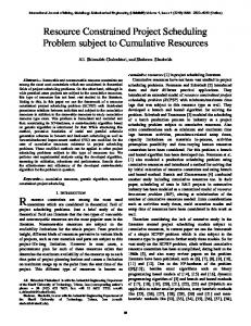
In this section we will compute the optimal solution by means of an instance adapted from the Patterson set (Patterson [12]). The corresponding AON project network is shown in figure 1. There are 7 activities (and two dummy activities) and one resource type with an availability of 5. The number above the node denotes the activity duration, while the numbers below the node denote the due date, the unit penalty cost (the unit earliness costs equals the unit tardiness costs) and the resource requirements, respectively. The branch-and-bound tree for the example is given in figure 2. At the initial level p = 0, the value of the optimal solution using the recursive procedure is lb = 5 with finishing times f2 = 4, f3 = 3, f4 = 6, f5 = 8, f6 = 6, f7 = 9 and f8 = 4. Since there is a resource conflict at time instant 1 caused by activities 2, 3 and 8, we determine the

188

VANHOUCKE ET AL.

Figure 1. A project network from the Patterson set.

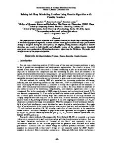
Figure 2. The branch-and-bound tree.

minimal delaying set at the next level of the branch-and-bound tree. DS = {{2}, {3}, {8}} and therefore, we create 6 delaying modes (with six additional precedence relations) corresponding to the six nodes at level p = 1. We compute for each node a lower bound by the recursive procedure for the unconstrained weighted earliness–tardinesss project scheduling problem. Now we select the delaying mode with the smallest lower bound, i.e., node 3 with lb = 15 and finishing times f2 = 4, f3 = 3, f4 = 6, f5 = 8, f6 = 6,


189

Figure 3. The optimal resource profile.

f7 = 9 and f8 = 6. Activities 4, 6 and 8 cause a resource conflict at time instant 5. We generate DS = {{4}, {6}} and 4 delaying modes corresponding to nodes 8, 9, 10 and 11 at the level p = 2. Remark that the solution of node 9 is resource feasible. We update the current upper bound ub = 27. We continue with the delaying mode with the smallest lower bound, i.e., node 8 with lb = 22 and finishing times f2 = 4, f3 = 3, f4 = 6, f5 = 8, f6 = 5, f7 = 9 and f8 = 6. Since the resource requirements at time instant 3 exceed the resource availibilities, the solution of this node is not resource feasible either. Again, we generate DS = {{2}, {6}} and 4 delaying modes corresponding to nodes 12, 13, 14 and 15 at level p = 3. Node 12 can be fathomed by node 10 due to the subset dominance rule (this is denoted by D10 in figure 2). We compute a lower bound for nodes 13, 14 and 15. All three nodes can be fathomed because the lower bound is greater than the current upper bound. The procedure now backtracks to level p = 2 and selects node 11 which has the smallest lower bound. The algorithm continues this way until it returns at the initial node at level 0. The optimal solution of the example has a weighted earliness–tardinesss cost of 27 as shown in node 9 of figure 2. The resource profile of the optimal solution is given in figure 3. Notice that an optimal solution with respect to the makespan objective does not necessarily correspond to the optimal solution of the RCPSPWET. The minimal makespan of this example is 8 while the optimal weighted earliness–tardinesss-schedule corresponds to a makespan of 9. 7.

Computational experience

Both the recursive search algorithm for the WETPSP and the branch-and-bound algorithm for the RCPSPWET have been coded in Visual C++ Version 4.0 under Windows NT 4.0 on a Dell personal computer (Pentium 200 MHz processor). In order to validate both algorithms, we used the problem generator ProGen/Max (Schwindt [13]) to generate two different problem sets. The first problem set for the WETPSP contains 1,680 problem instances while the second problem set for the RCPSPWET consists of 7,560 problem instances. The settings of these instances in activity-on-the-node format are described in the sequel of this paper.

190

VANHOUCKE ET AL.

Table 1 Parameter settings used to generate the test instances for the WETPSP. Number of activities Activity durations Number of initial and terminal activities Maximal number of successors and predecessors Order strength OS (Mastor [10]) Due dates Unit penalty cost

30, 60, 90 or 120 randomly selected from the interval [1,10] randomly selected from the interval [2,4] 4 0.25, 0.50 or 0.75 randomly selected with factor 1.00, 1.25, 1.50, 1.75, 2.00, 2.25 or 2.50 randomly selected from the interval [1,10] or [1,50]

Table 2 Impact of the number of activities. # activities

# problems

Average CPU-time

Standard deviation

30 60 90 120

420 420 420 420

0.075 0.289 0.585 1.043

0.042 0.162 0.296 0.628

Both problem sets were extended with unit penalty costs and due dates for each activity. The due dates were generated as follows: first, we obtained a maximum due date for each project by multiplying the critical path length with a factor as shown in table 1. Then we randomly generated numbers between 1 and the maximum due date. Finally, we sorted these numbers and assigned them to the activities in increasing order, i.e., activity 1 has the lowest due date, activity 2 the second lowest, etc. 7.1. Computational experience for the WETPSP Table 1 represents the parameter settings used to generate the test instances for the WETPSP. The parameters used in the full factorial experiment are indicated in bold. Using four settings for the number of activities, three settings for the order strength, seven settings for the due date generation and two settings for the unit penalty costs, we obtained a dataset with 168 problem classes, each consisting of 10 instances. Table 2 represents the average CPU-time and its standard deviation in milliseconds (actually, we have solved 1,000 replications for each problem and reported the time in seconds). Even instances with 120 activities can be solved within a very small amount of computation time. We should keep in mind that the unconstrained weighted earliness–tardinesss project scheduling problem is probably not a goal by itself. Its solution will be used by a branch-and-bound procedure to compute bounds on the weighted earliness–tardinesss cost of a resource-constrained weighted earliness–tardinesss problem where the activities are also subject to renewable resource constraints (problem m, 1|cpm|early/tardy). In that case the unconstrained problem should be solved efficiently in every (undominated) node of the branch-and-bound tree, which may run in the thousands (even millions). The reported CPU-times indicate that the recursive search


191

procedure may well be used for that end. Notice also the relatively small standard deviations, reflecting the rather robust behaviour of the procedure over the different problem instances. Table 3 shows a positive correlation between the OS of a project and the required CPU-time, i.e., the more dense the network, the more difficult the problem. Figure 4 illustrates the effect of the due date on the average required CPU-time. When the factor used for the due date generation is small, the problems contain many binding precedence relations and their solution will require an extensive search to shift many sets of activities SA to solve the problem. Problems with a large factor for the due date generation contain only few binding precedence relations in the due date tree. In that case, many activities will be scheduled on their due date and only a small number of shifts will be needed to solve the problem. As expected, the earliness and tardiness penalty costs of the activities have no significant impact on the required CPU-time, as shown in table 4. Table 3 Impact of the order strength. OS

# problems

Average CPU-time

Standard deviation

0.25 0.50 0.75

560 560 560

0.403 0.478 0.613

0.378 0.440 0.647

Figure 4. Effect of the due date. Table 4 Impact of the unit penalty cost. Unit penalty cost

# problems

Average CPU-time

Standard deviation

[0,10] [0,50]

840 840

0.495 0.501

0.508 0.510

192

VANHOUCKE ET AL.

7.2. Computational experience for the RCPSPWET Table 5 represents the parameter settings used to generate the test instances for the RCPSPWET. The parameters used in the full factorial experiment are indicated in bold. We obtained 756 problem classes, each consisting of 10 instances. Table 6 represents the average CPU-time and its standard deviation in seconds for a varying number of activities and a time limit of 100 seconds. The number of activities has a significant effect on the average CPU-time and on the number of problems solved to optimality, as displayed in table 6 and figure 5, respectively. All problems with 10 activities can be solved to optimality within 1 second of CPU-time. For problems containing 20 activities, 93.8% of the number of problems can be solved to optimality when the allowed CPU-time is 1 second, whereas 99.8% of the number of problems can be solved when the time limit is 100 seconds. For problems with 30 activities, 79.4% of the number of problems can be solved within 1 second of CPU-time whereas 90.8% of the number of problems can be solved to optimality when the allowed CPU-time is 100 seconds. The effect of OS on the number of problems solved to optimality is displayed in figure 6. As expected, the order strength has a negative correlation with the problem hardness, that is, the higher OS, the easier the problem. We have observed that for the WETPSP the opposite is true. That means that, although OS has a positive correlation with the problem hardness for the WETPSP, the overall effect for the RCPSPWET remains negative. Table 5 Parameter settings used to generate the test instances for the RCPSPWET. Number of activities Activity durations Number of initial and terminal activities Maximal number of successors and predecessors Order strength OS (Mastor [10]) Number of resource types Number of resources used per activity Activity resource demand Resource factor RF (Pascoe [11]) Resource strength RS (Kolish et al. [9]) Due dates Unit penalty cost

10, 20 or 30 randomly selected from the interval [1,10] randomly selected from the interval [2,4] 4 0.25, 0.50 or 0.75 4 randomly selected from the interval [1,4] randomly selected from the interval [1,10] 0.25, 0.50, 0.75 or 1.00 0.00, 0.25 or 0.50 randomly selected with factor 1.00, 1.25, 1.50, 1.75, 2.00, 2.25 or 2.50 randomly selected from the interval [1,10]

Table 6 Impact of the number of activities. # activities

# problems

Average CPU-time

Standard deviation

10 20 30

2520 2520 2520

0.001 0.508 11.391

0.006 4.128 29.962


193

Figure 5. Effect of the number of activities.

Figure 6. Effect of the order strength (OS).

Figures 7 and 8 display the effect of the resource factor (RF) and the resource strength (RS), respectively, on the number of problems solved to optimality within an allocated CPU-time. The higher the resource factor, the more difficult the instances. An opposite effect can be observed for the resource strength. The number of problems solved to optimality increases when RS increases. These results were also observed by Kolisch et al. [9] and De Reyck and Herroelen [2]. Table 7 illustrates the effect of the due date for a different number of activities on the CPU time with a time limit of 100 seconds. The negative correlation between the due date factor and the hardness of the problem is due to two reasons. First, this effect was also observed for the WETPSP: when the factor used for the due date generation is small, the problem contains many binding precedence relations and an extensive search will be needed to shift a large number of sets of activities to solve the problem. Problems with a large factor for the due date generation contain only few binding precedence relations

194

VANHOUCKE ET AL.

Figure 7. Effect of the resource factor (RF).

Figure 8. Effect of the resource strength (RS). Table 7 Impact of due date factor on the CPU-time.

10 activities 20 activities 30 activities

1.00

1.25

1.50

1.75

2.00

2.25

2.50

0.002 1.221 22.684

0.002 1.103 17.135

0.001 0.723 12.508

0.001 0.212 9.828

0.001 0.139 7.651

0.001 0.107 5.455

0.001 0.05 4.475

in the due date tree. In that case, many activities will be scheduled on their due date and only a small number of shifts will be needed to solve the problem. Second, when the due date factor is large, the number of nodes in the search tree will decrease dramatically since the probability of a resource conflict will decrease. Both the number of nodes in the search tree and the time spent per node are negatively correlated with the due date factor.


195

Table 8 Impact of the subset dominance rule on the number of subproblems solved.

10 activities 20 activities 30 activities

With dominance rule

Without dominance rule

78 20,992 355,358

89 23,813 414,560

Table 8 shows the effect of the subset dominance rule on the average number of nodes in the search tree without exceeding a time limit of 100 seconds. In each node a call to the recursive search algorithm is performed to solve the WETPSP. The table reveals that the subset dominance rule reduces the number of subproblems solved during the search process with, on the average, 14%. 8.

Conclusions

In this paper, we presented a branch-and-bound procedure for the resource-constrained project scheduling problem with weighted earliness–tardinesss penalty costs (RCPSPWET; m, 1|cpm|early/tardy) based on a fast exact recursive search algorithm for the unconstrained weighted earliness–tardinesss problem (WETPSP; cpm|early/tardy). Activities have a known deterministic due date, a unit earliness as well as a unit tardiness penalty cost and renewable resource requirements. The objective is to schedule the activities in order to minimize the total weighted earliness–tardinesss penalty cost subject to both the precedence and resource constraints. To the best of our knowledge, our procedure is the first exact algorithm for solving the RCPSPWET. The branching strategy of the depth-first branch-and-bound algorithm makes use of a fast recursive search algorithm for the unconstrained weighted earliness–tardinesss problem to compute the lower bounds. The resource conflicts are solved by generating minimal delaying alternatives and by introducing extra precedence relations. A subset dominance rule is used for additional node fathoming. Both the recursive search procedure for the WETPSP and the branch-and-bound procedure for the RCPSPWET have been coded in Visual C++, version 4.0 under Windows NT and have been validated on a randomly generated problem set generated by ProGen/Max (Schwindt [13]). The results of the extensive computational tests obtained on a Dell personal computer (Pentium 200 MHz) are rather encouraging. The results for the WETPSP reveal that the recursive search algorithm is very fast which makes it very useful for the calculation of a lower bound in the branch-and-bound procedure for the RCPSPWET. The results for the RCPSPWET are promising. Although the number of activities is found to have a significant effect on the required average CPU-time and the number of problems solved to optimality, the procedure is rather robust. Problems with 30 activities can be solved in an average CPU-time of 11 seconds (some 80% of the problems can be solved within 1 second of CPU-time; while this percentage goes up to 90% when the CPU-time allowance is increased to 100 seconds). An investigation

196

VANHOUCKE ET AL.

of the impact of the topological structure of the network reveals that problems become easier to solve as the order strength goes up. The higher the resource factor, the more difficult the problem. An opposite effect has been observed for the resource strength. The tighter the due date, the more difficult the problem. The subset dominance rule allowed to fathom on the average 14% of the nodes in the search tree. The procedure holds the promise to handle other types of nonregular objective functions (such as the maximization of the net present value of the project) with similar performance. References [1] B. De Reyck, Scheduling projects with generalized precedence relations, exact and heuristic procedures, Ph.D. Dissertation, Katholieke Universiteit Leuven, Belgium (1998). [2] B. De Reyck and W. Herroelen, A branch-and-bound procedure for the resource-constrained project scheduling problem with generalized precedence relations, European Journal of Operational Research 111 (1996) 125–174. [3] B. De Reyck and W. Herroelen, An optimal procedure for the resource-constrained project scheduling problem with discounted cash flows and generalized precedence relations, Computers and Operations Research 25 (1998) 1–17. [4] E. Demeulemeester and W. Herroelen, A branch-and-bound procedure for the multiple resourceconstrained project scheduling problem, Management Science 38 (1992) 1803–1818. [5] E. Demeulemeester and W. Herroelen, New benchmark results for the resource-constrained project scheduling problem, Management Science 43 (1997) 1485–1492. [6] W. Herroelen, P. Van Dommelen and E. Demeulemeester, Project network models with discounted cash flows: A guided tour through recent developments, European Journal of Operational Research 100 (1997) 97–121. [7] W. Herroelen, E. Demeulemeester and B. De Reyck, A classification scheme for project scheduling problems, in: Project Scheduling Recent Models, Algorithms and Applications, ed. J. W¸eglarz (Kluwer Academic, 1999) pp. 1–26. [8] O. Icmeli and S.S. Erengüç, A branch-and-bound procedure for the resource-constrained project scheduling problem with discounted cash flows, Management Science 42 (1996) 1395–1408. [9] R. Kolisch, A. Sprecher and A. Drexl, Characterization and generation of a general class of resourceconstrained project scheduling problems, Management Science 41 (1995) 1693–1703. [10] A.A. Mastor, An experimental and comparative evaluation of production line balancing techniques, Management Science 16 (1970) 728–746. [11] T.L. Pascoe, Allocation of resources – CPM, Revue Française de Recherche Opérationelle 38 (1966) 31–38. [12] J.H. Patterson, A comparison of exact procedures for solving the multiple resource-constrained project scheduling problem, Management Science 30 (1984) 854–867. [13] C. Schwindt, A new problem generator for different resource-constrained project scheduling problems with minimal and maximal time lags, WIOR-Report-449, Institut für Wirtschaftstheorie und Operations Research, University of Karlsruhe, Germany (1995). [14] M. Vanhoucke, E. Demeulemeester and W. Herroelen, An exact procedure for the unconstrained weighted earliness–tardinesss project scheduling problem, Research Report 9907, Department of Applied Economics, Katholieke Universiteit Leuven, Belgium (1999).