IEEE TRANSACTIONS ON APPLIED SUPERCONDUCTIVITY, VOL. 14, NO. 2, JUNE 2004
1317
Target Field Approach for Spherical Coordinates Ye Bai, Qiuliang Wang, Yunjia Yu, and Keeman Kim
Abstract—Using the method of separation of variables and expanding the magnetic field generated by currents flowing on a sphere by means of Fourier-Legendre expansion, we can obtain the inverse relationship between the current density and magnetic flux density. The current density required to generate a specified target field inside the sphere may be evaluated. This approach develops Turner’s target field method and can generate axially directed field in large usable volumes inside the sphere, which can satisfy the requirement of high-energy physics, medical treatment, spatial detection etc. Using this method we can generate uniform or gradient magnetic field that vary linearly along the z or y direction. The commercial finite element method software also verifies the validation of this approach. Index Terms—Gradient field, spherical coils, stream function, target field approach.
I. INTRODUCTION
I
N FUSION research, high-energy physics, particle accelerators, space detectors and medical imaging devices [1], we often need to generate specific magnetic field in spatial positions according to its application. This type of problem belongs to an inverse method that leads to design the shape of coils knowing the magnetic field distribution. The design of gradient coil is the most common problem. There are two methods of designing gradient coils. One is to adjust the coil position by means of optimum methods step by step until an acceptable design is obtained. Although it is easy to apply for an arbitrary shape of coils, this method has the disadvantage to require heavy mathematical calculations and an exhaustive research of global optimum result. The other method is called the target field approach [2] that was originally discussed by Turner. It is a noniterative technique which sets predetermined values of magnetic flux density at given spatial positions, and then uses the inverse calculating method to calculate a find back desired current density distribution. Finally by applying the stream function technique to the continuous current distribution, we can generate the discrete current pattern. This approach is mathematically based on Fourier-Bessel expansion of the magnetic field generated by current, thus the relationship between current and field may be inverted. The most typical gradient coil geometry is a cylindrical one where the target field method was used at first. The disadvantages of cylindrically shaped gradient coils are high levels of the dissipated magnetic energies leading to higher values of inductances. Since the stored magnetic energy is proportional to
the fifth power of the coil radius, more compact geometries are preferable, such as the biplanar, elliptical, and spherical coils. In some applications we need to generate specific magnetic field over a spherical volume such as in high-energy physics and MRI [3]. The ideal situation is the spherical coil geometry. In comparison with the cylindrical coils, the spherical coils have the advantage of smaller values of inductances, lower energy storage and less magnetic flux leakage. In Turner’s article, the target field method is used in cylindrical or shim coils’ design. The subject of generation magnetic field over a spherical volume was studied only by a few researchers. In this paper, Turner’s approach is developed and used in the design of spherical coils. This approach allows the modeling of particular uniform or gradient magnetic fields inside the sphere. II. FORMULAS OF SPHERICAL COORDINATES In source-free region, the magnetostatic field sented as:
In spherical coordinates, Laplace equation be written as:
can be repre-
, can
(1) Using the method of separation variables, we find the expresto be [4]: sion for
(2) To find the magnetic field everywhere, we first note that the field outside the sphere must decay as and the field . Therefore the field inside the sphere must be finite as outside the sphere can be represented by:
Manuscript received October 20, 2003. Y. Bai, Q. Wang, and Y. Yu are with the Institute of Electrical Engineering Chinese Academy of Sciences, Beijing, CO 100080 China (e-mail:
[email protected]). K. Kim is with Korea Basic Science Institute, Taejon, Korea. Digital Object Identifier 10.1109/TASC.2004.830565 1051-8223/04$20.00 © 2004 IEEE
(3)
1318
IEEE TRANSACTIONS ON APPLIED SUPERCONDUCTIVITY, VOL. 14, NO. 2, JUNE 2004
and the field inside the sphere can be represented by: (14) The value of z component of magnetic flux density inside the sphere can be written as: (15) The associated Legendre functions are subject to the following recurrent relationship [6]: (4) As we can see, the three respective directions component , , and . values are: The boundary conditions across the spherical surface are as follows:
(16) Substituting (4), (16) into (15), multiplying both sides of (15) and then integrating it from 0 to with respect to , by we get:
(5) After vector calculation, (5) can be written as[5]: (6) (7) (8) Substituting (3), (4) into (6), (7), (8) and multiplying both and then integrating it from 0 to sides of (7) and (8) by with respect to [2], we get:
(9)
(17) The associated Legendre functions are also subject to the following orthogonal relationship [6]:
(18) Considering the orthogonal relationship (18), we substitute (12) into (17), multiply both sides of (17) by and then integrate it from 0 to with respect to . After simplification, we finally obtain an important relationship: (19) where
(10)
(20)
The associated Legendre functions are subject to the following orthogonal relationship [6]:
Equation (19) is the general Fourier transform relationship between the axially z-directed field inside the sphere and the spherical surface current density. The value of y component of magnetic flux density inside the sphere can be written as: (21) By means of a similar derivation method, we can obtain the following relationship:
else. Using (9), (10) and (11) we finally obtain [7]:
(11) (22) (12)
where
where
(23) (13) and
,
are as defined earlier.
BAI et al.: TARGET FIELD APPROACH FOR SPHERICAL COORDINATES
1319
According to the above derivation, the general principles of this approach is first to specify a desired magnetic field inside the spherical volume, then using (19) or (22) to obtain the general Fourier transform of the surface current density. At last, we can perform the general inverse Fourier transform to find the and on the sphere. desired surface current values of III. FORMULAS APPLICATION We assume the desired distribution of the z component of magnetic flux density to be
that means a uniform magnetic flux density. represents the value of the current density. According to (13), (14), (18), (19) and (20) we can finally obtain:
Resorting to the above results and (22), (23), we also obtain
Another example is to assume the desired gradient field along the z-axis as
Fig. 1.
Distribution of flux lines inside the sphere.
Then by integrating the expression over the line segments, we determine the position component of the individual loops as: (25) The number of wires in each region is determined using the relation:
Applying the same technique we finally get:
By means of the above method, we can generate spherical coils that are capable of producing an axially directed field, that is uniform or vary linearly along the z direction or y direction. This conclusion can also be partly verified from [5]. IV. DISCRETE APPROXIMATION OF THE CONTINUOUS CURRENT DENSITY Following the target field approach, the outcome is the continuous current distribution for the spherical coils. In order to get the actual axially uniform or gradient coils, we must generate the discrete current distribution patterns to fabricate the coils. To use this method we must know information about the number of the individual current loops in each section, their position relative to the center of the sphere and the magnitude of the current in the current loops. This is feasible by using the stream function technique that was originally presented by W. A. Edelstein [8]. Since the current density satisfies the continuity equation, there exists a vector function , such that
In the case of spherical coils mentioned above, the current density is confined to lie on the surface of the sphere and is directed along the direction. Expressing the curl of a vector in spherical coordinates, we obtain: (24)
where (26) stands the whole number of the current loops on the sphere surface, which is determined before the coil’s construction. Symbol means the magnitude of a current loop. Using this method, we can use discrete coils to substitute the continuous current density on the sphere surface. Although it will bring out some errors, we can diminish them by increasing the current loops. V. VERIFICATION OF THE APPROACH BY FINITE ELEMENT METHOD To verify this approach we used a commercial finite element method analysis software [9] to simulate the spherical coils mentioned above. For succinctness only a semi sphere is shown. Fig. 1 shows the flux lines inside the sphere generated by the current density
on the surface of the sphere. The z component of flux density inside the sphere is shown in Fig. 2. As we can see, the z-axis uniform magnetic field has been generated. Because the y component of flux density is zero, we do not plot this figure.
1320
IEEE TRANSACTIONS ON APPLIED SUPERCONDUCTIVITY, VOL. 14, NO. 2, JUNE 2004
Fig. 2. Z-axis uniform field B inside the sphere.
Fig. 3. Distribution of flux lines inside the sphere.
Fig. 3 shows the flux lines inside the sphere generated by the current density
on the spherical surface. The z and y components of the flux density inside the sphere are shown in Figs. 4 and 5. As clearly shown, we can generate gradient field that vary linearly along the z-axis and y-axis inside the sphere.
Fig. 4.
Z-axis gradient field B inside the sphere.
Fig. 5.
Y-axis gradient field B
inside the sphere.
the sphere surface by the means of discrete coils. This technique is appropriate for engineering design. In particle accelerators, electron beam devices, source for biasing fields and today’s ultra fast MRI applications, a highly uniform or linearly gradient field is often required in a spherical volume. The method, described in this article, develops Turner’s target field approach and can greatly simplify the design process of spherical coils. Finally, we use the commercial finite element method software ANSOFT to verify this approach and obtain satisfactory simulating results. NOMENCLATURE
VI. CONCLUSION The target field approach for spherical coordinates provides a powerful tool in the design of spherical coils. Applying an inverse calculating method, given the z or y component of magnetic flux density inside the sphere we can obtain the surface current density on the sphere. Then by using the stream function technique, we substitute the continuous current density on
Symbols
Quantity SI Magnetic scalar potential. [A] Arbitrary constants to be determined by specific problems. Arbitrary constants to be determined by specific problems. Associated Legendre Function.
BAI et al.: TARGET FIELD APPROACH FOR SPHERICAL COORDINATES
Vector of Magnetic flux density. [T] Magnetic permeability of free
1321
space.
Unit vector along the radial direction. Unit vector along the direction. Unit vector along the direction. Radius of the sphere [m] Column matrix of flux density components. [T] Unit vector defining the normal direction of sphere. Vector of current density. component of current density. component of current density. Dirac’s symbol. Hamilton operator. General Fourier transform of . General Fourier transform of . General Fourier transform of . Derivative of associate Legendre polynomial.
General Fourier transform of Vector stream function Number of wires in each region Value of the current function in each region Desired magnitude of the current in the loop [A] REFERENCES [1] D. I. Hoult et al., “Electromagnet for nuclear magnetic resonance imaging,” Rev. Sci. Instrum., vol. 52, no. 9, pp. 1342–1351, Sept. 1981. [2] R. Turner, “A target field approach to optimal coil design,” J. Phys. D, Appl. Phys, vol. 19, pp. 147–151, 1986. [3] H. Liu and L. S. Petropoulos, Spherical Gradient Coil for Ultrafast Imaging, vol. 81, no. 8, pp. 3853–3855, Apr. 15, 1997. [4] K. M. Liang, “Math physics method,” in Higher Education Press, 3rd ed., Jun. 1978. [5] R. S. Elliot, Electromagnetic. New York: McGraw-Hill, 1966. [6] M. Abramowitz and I. Stegun, Handbook of Mathematical Functions, Washington: National Bureau of Standards, reprinted by New York: Dover Publications, 1968. [7] W. C. Chew, Waves and Fields in Inhomogeneous Media. New York: IEEE Press, 1995, p. 187. [8] W. A. Edelstein and F. Schenck, “Current Streamline Method for Coil Construction,” U. S. Patent 4 840 700, 1989. [9] ANSOFT User’s Manuals and Procedures Guides Revision 7.0, ANSIOFT Inc., Pittsburgh, PA, 1998.