Technical note: Querying SQLite databases in R Stuart K. Grange∗a,b a
School of Environment, the University of Auckland, Auckland, New Zealand
b School
of Population Health, the University of Auckland, Auckland, New Zealand
September 4, 2014
1
Introduction
R is a free and open-source statistical programming language which has exploded in popularity and is ideal for many statistical and numerical computing applications.[1,2] The first step for almost any analyses undertaken in R, or any other statistical/numerical environment, is getting data read and loaded into the application. In many situations this will involve the use of relational databases. The term ‘database’ is used in many situations and its definition is ambiguous. However, in this note, the database definition is one which is concerned with relational databases which are nearly always interacted with the use of SQL (Structured Query Language).[3,4] 1.1
Relational databases and SQL
Relational databases are a collection of things, generally rectangular data tables which have been designed to be related to one another.[4] Relational databases are often used when the storing of data in a ‘flat’ form creates too much redundancy, when it becomes impractical to read and load an entire dataset at once, or when there are multiple users of the same dataset. Relational databases are almost always discussed alongside SQL. SQL does not refer to the database itself, rather a specialised programming language which allows a data user to manipulate the database with intuitive verbs.[4] However, rather confusingly, many database systems contain SQL in their name because it is a critical piece of the database’s design. Many programming languages, such as R, allow you to use the SQL language directly, or indirectly within them so databases can be used easily and efficiently.[5] Relational databases can be extremely useful when subsets of an entire dataset want to be looked at or when there are many different observational units which are impractical to store as a single table. For example, I am an air quality scientist and I generally deal with large amounts of time-series data. Air quality data is usually stored as hourly averages (if the instrumentation allows) and sites are often online for decades. When we consider ∗
[email protected]
1
that a city, region, or country has many monitoring sites (in some situations hundreds), dealing with this amount of data quickly becomes unwieldy. Most data users attempt to keep subsets of the data to avoid confusion and manage work-flow. However, it is often useful, or necessary, to compare sites, times, and pollutants with one-another and this cannot be done conveniently if pieces of the data are separate and stored in different files and in different locations. Furthermore, there is often some amount of ‘metadata’ such as site features and descriptions, site history, service information, and instrumentation details which can be extremely useful to have easy access to when analysing pollutant concentrations. Relational databases allow for a tidy and efficient way to deal with these sorts of (and many other) data issues. 1.2
The usage of relational databases
The mechanics of using relational databases are different than other data types such as plain text files or Microsoft Excel workbooks. Rather than opening or reading a file and then doing something with it, the database is first connected to, and then it is queried. A database query tells the database service to do something, and for data users, this is usually the retrieval of data. These database queries are almost always written in SQL. Queries range from being simple, such as returning the entire contents of a single data table, to complicated versions where multiple matches are desired and multiple tables are joined together in some fashion. For most data users, the most relevant SQL verbs are SELECT, FROM, WHERE, BETWEEN, and JOIN. For database management, there are other verbs such as DELETE and INSERT which can be used too. DELETE and INSERT cannot be considered as querying verbs however, rather manipulation verbs. To explain how these SQL verbs work, a few examples using an air quality database will be given in this note. Basic knowledge and usage of R is assumed, but the examples discussed are simple so this note maybe able to be used as an R introduction too. 1.3
The example SQLite database
The database which will be used as an example is a SQLite database which contains hourly atmospheric pollutant and meteorological data from 26 monitoring locations in and around the Lower Fraser Valley, British Columbia, Canada. The source of these data is the British Columbia air quality data website (http://envistaweb.env.gov.bc.ca/). These data required a moderate amount of cleaning and tidying before being transformed into a database. These ‘data-wrangling’ steps will not be discussed here. SQLite is the simplest implementation of a relational database and it has numerous drawbacks when compared to some other databases. Some of these limitations will be encountered in this note. However, critically, a SQLite database is contained within one file and this file is as portable as a .pdf or .txt file. This allows SQLite databases to be moved around and shared with others easily which I believe is a huge advantage over the more complex, bonafide client-service models used by other databases such as MySQL and PostgreSQL which usually require dedicated systems, and other technical skills to set-up. 2
1.4
Objectives
This note’s primary objective is to get data users familiar to using SQL within R quickly so they can use databases they have encountered, or have already received. Although the example database which will be used is a SQLite version, the commands and philosophy are similar for other relational database types. 1.5
Set-up and dependences
The use of relational databases with R requires additional packages to be loaded. The DBI package is the main database driver for R, and extensions are necessary to interact with a specific type of database.[5] The RSQLite package will be used in this note and the installation of this package will force R to install DBI.[5,6] There will also be dependence on the openair, plyr, lubridate, ggplot2, and stringr packages.[7,8,9,10,11,12] If these are not installed on your system, I would recommend that this is done before tackling the following examples. Also notable is that this document has been produced with knitr[13] and the code chunks will display the steps discussed within the note, for example: # Let's load the packages which will be used # A package for SQLite usage library(RSQLite) ## Loading required package:
methods
## Loading required package:
DBI
# A package for air quality data analysis library(openair) # Plotting library(ggplot2) # A packages which makes working with dates easy library(lubridate) # A package which allows split-apply-combine analyses to be done easily library(plyr) ## ## Attaching package:
’plyr’
## ## The following object is masked from ’package:lubridate’: ## ##
here
# Make string processing constant library(stringr)
3
2
Creating a database connection
The first step of working with a SQL relational database is connect to it with the dbConnect function. In the case of SQLite, the database is a single file so it is intuitive how this is done. In this example, the database has the .sqlite extension but often they take the file-form .db. # The RSQLite package has been loaded # Now connect to the database file.name = 2005.
10
Jan
Apr
Jul
bkp
bmt
ha
rob
Oct
80 60 40 20
O3
0
80 60 40 20 0 Jan
Apr
Jul
Oct
O3
Figure 2: Hourly ozone data for four sites in the Lower Fraser Valley, British Columbia for 2005.
11
4.3
Joining different tables with JOIN
Figure 2 looks good, but the conditioning variable, site, is rather opaque and not very clear. It would be better if these plots had the sites’ full names and their surrounding landuse zones for presentation purposes. As shown in Section 3, the table named data does not contain these variables; but the info_sites table does. SQL queries can be built which combines or joins tables together and returns variables/columns from each separate observational unit. Joins like this demonstrate the relational model which SQL databases are based upon. For joins to be possible, we need common variables among the different tables which can be matched and these are usually called the key variables. To command a SQL database to return columns from different tables, we use the verb JOIN. There are a few usages of JOIN but we will use the version with no extra arguments which is equivalent to an INNER JOIN. # Select ozone, data, and site data from the table named data # and join the sites' names and landuse zone with site as the key # variable data.o3