Technique for 3D shape reconstruction of spherical and aspheric

EPJ Web of Conferences 48, 00016 (2013) DOI: 10.1051/epjconf/20134800016 © Owned by the authors, published by EDP Sciences, 2013

Technique for 3D shape reconstruction of spherical and aspheric surfaces using deflectometric principle A. Mikš, J. Novák, and P. Novák Czech Technical University in Prague, Faculty of Civil Engineering, Department of Physics, Thakurova 7, 16629 Prague, Czech Republic

Abstract. We provide a description and analysis of a deflectometric technique for 3D measurements of optically smooth surfaces. It is presented that a surface reconstruction problem leads to a theoretical description by a nonlinear partial differential equation. Then, a surface shape can be calculated by solution of a derived equation. The presented method is noncontact and no reference surface is needed as in interferometry.

1 Introduction Various methods were developed for surface topography measurements in recent years, which find many applications in different parts of science, engineering, and biomedicine. The existing measurement and evaluation methods are based on different physical principles. Generally, it is possible to divide these methods into contact 1,2 and noncontact techniques 2-8. One type of optical methods is based on deflectometry 7,9-15, which is used frequently for noncontact surface measurements. This work presents a deflectometric approach to solving a 3D surface reconstruction problem, which is based on measurements of a surface gradient of optically smooth surfaces. It is shown that a description of this problem leads to a nonlinear partial differential equation, from which the surface shape can be reconstructed numerically. The reconstruction process is presented on an example.

vector n of the surface normal in the point P(x,y,z). After the reflection from the surface the ray intersects the plane  in the point Q, which is located in the distance t from the point C. The distance t = t(x,y) depends on the position of the point P(x,y,z) at the measured surface. The direction of the reflected ray is characterized by the unit vector s' and the angle ' with respect to the unit surface normal vector n.

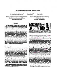
2 Description of surface reconstruction Consider an optical surface, mathematically described by the formula z  f ( x, y) . The principle of the gradient deflectometric method is shown in figure 1, where O is the origin of a chosen coordinate system and P(x,y,z) is a point at the surface. Further, assume that the axis z is perpendicular to the plane , which is located at the distance a from the plane xy. The ray described by its unit direction vector s, which is parallel to the z axis, intersects the plane  in the point C and the measured surface in the point P(x,y,z). The incidence angle  is defined as an angle between the direction vector s and the unit

Fig.1. Principle of deflectometric method

Corresponding to the law of reflection the vectors s, s' and n as well as the points P, C and Q lie in one plane. It holds due to the reflection law 16,17

s  s  2n(sn) and

cos   sn ,

(1)

   .

(2)

We obtain for the normal vector 17

This is an Open Access article distributed under the terms of the Creative Commons Attribution License 2.0, which permits unrestricted use, distribution, and reproduction in any medium, provided the original work is properly cited. Article available at http://www.epj-conferences.org or http://dx.doi.org/10.1051/epjconf/20134800016

EPJ Web of Conferences where

s  s

n

21  (ss)

.

(3)

 ( x, y , z )  b  b 2  1 2

 1  2 / K  2 1  1/ K / K

Corresponding to figure 1 we can write

t PC

t 2 tan  .  tan 2  az 1  tan 2 



z , x

q

z . y

(5)

3 Analysis and examples

Then, it is well known that the unit normal vector to the surface z  f ( x, y) can be expressed as 18,19

q 1  p n   ,  ,  , N N  N

Figure 2 presents a principal scheme of a possible technical realization of the sensor head for the measurement of distance t. The ray with the direction vector s propagates through the semitransparent mirror M and reflects at the measured surface S ( x, y, z )  0 in the point P. The reflected ray, which is characterized by the direction vector s, is reflected by the mirror M and intersects the plane of the CCD sensor in the point Q. The position of the point Q is evaluated and the distance t of the point Q from the center of the sensor C can be determined.

(6)

where N  1  p 2  q 2 . Assuming that the direction vector s of the incident ray is identical with the z axis direction, then

s  (0,0,1) .

(15)

The nonlinear partial differential equation of the first order (14) is a general solution of the problem of the reconstruction of the surface z  f ( x, y) using the deflectometric method. Due to the fact, that the general solution of Eq.(14) cannot be found in an explicit form, equation (15) must be solved numerically 18-19.

(4)

Moreover, we denote the derivatives of the function z  f ( x, y) as

p

2

(7)

and we obtain from previous equations

tan 2  

2 p2  q2 1  p2  q2

.

(8)

By substitution of previous formula into Eq.(4) we have

K

2 p2  q2 t  . az 1 p2  q2

(9)

Equation (11) can be also written in the form

K (1  p 2  q 2 )  2 p 2  q 2 .

(10)

By squaring the previous equation we can write the final equation ( p 2  q 2 )2  2b( p 2  q 2 )  1  0 , (11) where we denoted b  (1  2 / K 2 ) . (12)

Fig.2. Principal scheme of measuring sensor

During the measurement the surface is scanned and the distance t(x,y) is measured for different scanned points at the surface. The measuring process leads to a solution of a nonlinear partial differential equation of the first order 2

 z   z  F ( x, y )        x   y 

The solution of Eq.(14) has the following form

p 2  q 2  b  b2  1 .

(13)

2

(16)

 (1  2 / K 2  2 1  1 / K 2 / K )  0, where

Equation (13) can be generally expressed in the form

K

2

 z   z        ( x, y, z ) ,  x   y 

2

(14)

00016-p.2

t . az

(17)

Optics and Measurement 2012 To find a solution z  f ( x, y) of Eq.(16), the unknown function z  f ( x, y) can be expressed in the form of twodimensional polynomials, for example M

z  f ( x, y ) 

z  f ( x, y ) 

N

 c

mn x

m

y . n

(18)

m 0 n 0

M

 M

q

N

z  mc mn x m1 y n , x m0 n0

z (19)

N

z nc mn x m y n1 .  y m0 n 0



p

q

ik (c 00 , c10 , c 01 , c 20 , c11 , c 02 ,.....) .

(21)

5

 c (x s

2

 y2 )s .

(22)

(20)

i 1 k 1

The goal is to find such values of unknown coefficients cmn in order the function (20) was minimized. Different optimization techniques can be used of the mentioned optimization problem. Knowing coefficients cmn one can calculate coordinates ( xi , y k , z ik ) of the measured surface. A general problem of mathematical optimization techniques is a strong dependence on the starting point (initial values of coefficients cmn ). In many cases these method will not converge. However, in the case of testing spherical or rotationally symmetrical aspherics, which are fabricated in optics industry, one knows the nominal shape of the test surface very-well and thus a good starting point for the optimization procedures can be found. As an example we present a numerical simulation of the described reconstruction method for the case of a spherical shape surface. Consider that the radius of the spherical surface is R = - 50 mm, x   20, 20 ,

y   20, 20 . The step of the changes in coordinates x and y are chosen as x  1 mm and y  1 mm . For the

z  x

z  y

5

 2sxc ( x

2

s

 y 2 ) s 1 ,

s 1

(23)

5

 2syc ( x s

2

 y 2 ) s 1 .

s 1

As a starting point for the optimization we choose a parabolic surface with the following coefficients: c1  1 / 80 , c2  c3  c4  c5  0 . By solving a given optimization problem (20) we obtain c1 = -1.0000e-02, c2 = -9.9839e-07, c3 = -2.0762e-10, c4 = -3.3223e-14, c5 = -3.0350e-17.

K

 F

.

The derivatives with respect to x and y are given by

value t ( xi , y k ) is measured using the detector ( i  1,2,...,I , k  1,2,...,K ). By substitution into (16)(19), we obtain values Fik (c00 , c10 , c01, c20 , c11, c02 ,.....). We can create, for example, the following merit function for the formulation of the optimization problem I

1  1  c2 (x2  y 2 )

s 1

Other possibility is to use different type of polynomials (e.g. Legendre or Zernike polynomials) or the rotationally symmetrical aspheric surface description [5]. By the substitution of derivatives of the chosen function z  f ( x, y) into differential equation (16), we obtain the optimization problem instead of the solution of the partial differential equation. The measured area of the surface can be discretized into a grid of points ( xi , yk ) , where the

F

c( x 2  y 2 )

where c  1/ R is the surface curvature. The approximation polynomial for z coordinate is chosen in the form

One can calculate derivatives with respect to x and y as

p

simplicity, we chose a = 0. The spherical surface can be described by the following formula

Figure 3 presents the shape of the surface. Figure 4 shows an approximation error of the shape using the coefficients obtained from the solution of the optimization procedure.

Fig.3. Shape of surface

The proposed measurement method and the approach to find the solution of the partial differential equation (16), which describes theoretically the problem of surface reconstruction, give very good results and can be principally used for measurements of spherical and aspheric surfaces.

00016-p.3

EPJ Web of Conferences 8. 9. 10. 11. 12. 13. 14. 15. Fig.4. Approximation error of surface shape

16. 17. 18.

4 Conclusion The previous theoretical analysis and numerical simulations had shown that a general solution of the 3D shape reconstruction of the optical surface is given by a nonlinear partial differential equation of the first order, which is a completely original mathematical approach in surface topography. The shape of the measured surface can be numerically calculated from the derived equation. We presented a possible mathematical technique for the solution of the derived differential equation. We performed a numerical simulation of the presented method, which confirmed a good possibility for measurements and reconstruction of the shape of spherical and aspheric surfaces.

19.

Acknowledgment This work has been supported by the grant FR−TI2/074 of the Ministry of Industry and Trade of the Czech Republic.

References 1. 2. 3. 4. 5. 6. 7.

J.A.Bosch, Coordinate Measuring Machines and Systems, (CRC Press, 1995). D.J.Whitehouse, Handbook of Surface and Nanometrology, (Institute of Physics Publishing, 2003). T.Yoshizawa, Handbook of Optical Metrology: Principles and Applications, (CRC Press, 2009). F.M.Santoyo, Handbook of Optical Metrology, (CRC Press, 2008). D. Malacara, Optical Shop Testing, (John Wiley & Sons, 2007). J. Geng, Adv. Opt. Photon. 3, 128-160 (2011). R.Leach, Optical Measurement of Surface Topography, (Springer, 2011).

00016-p.4

A.Mikš, J.Novák, P.Novák, Proceedings of SPIE 6609 (2007). T. Bothe, W. S. Li, C. von Kopylow, W. Juptner, Proc. SPIE 5457 (2004). M. Knauer, J. Kaminski, G. Häusler, Proc. SPIE 5457 (2004). Y. Tang, X. Su, Y. Liu, H. Jing, Opt. Express 16, 15090-15096 (2008). M.Rosete-Aguilar, R. Díaz-Uribe, Appl. Opt. 32 (1993). W.D. van Amstel, S.M. Bäumer, J.L. Horijon, Proc. SPIE 3739 (1999). I. Weingärtner, M. Schulz, C. Elster, Proc. SPIE 3782 (1999). M. Schulz, G. Ehret, A. Fitzenreiter, J. Europ. Opt. Soc. Rap. Public. 10026, 5 (2010) M. Herzberger, Modern Geometrical Optics, (Interscience, 1958). A. Mikš, P. Novák, J. Opt. Soc. Am. A 29, (2012). K.Rektorys, Survey of Applicable Mathematics, (M.I.T. Press, 1969). G.A.Korn, T.M.Korn, Mathematical Handbook for Scientists and Engineers, (Courier Dover Publications, 2000).