Techniques for efficient covariance propagation in the ...

Techniques for efficient covariance propagation in the Extended/Unscented Kalman Filter based on model reduction

Frode Rønneberg

Master of Science in Engineering Cybernetics (2) Submission date: May 2013 Supervisor: Lars Imsland, ITK

Norwegian University of Science and Technology Department of Engineering Cybernetics

NTNU Norwegian University of Science and Technology

Faculty of Information Technology, Mathematics and Electrical Engineering Department of Engineering Cybernetics

MSc THESIS DESCRIPTION SHEET Name: Department: Thesis title:

Frode Rønneberg Engineering Cybernetics Techniques for efficient covariance propagation in the Extended/Unscented Kalman Filter based on model reduction

Background Even though the (recursive) EKF/UKF are considered efficient algorithms for state estimation, it can still be computationally expensive for medium to large systems. The bulk of the complexity stems from the propagation of the state covariance. In this task, the student will consider using techniques from model reduction to make the covariance propagation more efficient, while the full model still is used for state propagation. Work description 1. Literature study on EKF and UKF, and model reduction for nonlinear systems. 2. What is the complexity of covariance propagation? Perform a literature study on existing efficient filtering methods. 3. Suggest methods for efficient covariance propagation in the EKF and UKF based on a reduced model, while the full model is used for state propagation. 4. Implement for selected test systems. 5. (Compare with other methods for efficient estimation.) 6. Evaluate and discuss. Start date: January 14, 2013 Supervisor: Co-advisor(s):

Lars Imsland

Due date: June 10, 2013

Sammendrag Fysiske prosesser gir ingeniører og forskere utfordrende oppgaver som modellering, simulering og regulering. Ett av de viktigste stegene i disse prosessene er muligheten til ˚ a beregne fremtidig oppførsel, som ofte kan være en beregningsmessig kompleks og krevende oppgave. For høy kompleksitet i prosessene kan føre til at nødvendig informasjon beregnes for sent, gi avbrudd i produksjonssystemer, tap av kostnader, eller det som verre er, tap av liv. Dermed er det ˚ a finne mer effektive m˚ ater ˚ a estimere oppførselen til fysiske prosesser av spesiell interesse. Denne rapporten presenterer en ny fremgangsm˚ ate for tilstandsestimering ved ˚ a redusere beregningene i Extended Kalman Filter (EKF) og Unscented Kalman Filter (UKF) ved hjelp av teknikker fra modellreduksjon. Ved ˚ a redusere de mest krevende operasjonene, gitt av kovarianspropageringen i EKF og kalkuleringen av sigmapunktene i UKF, samtidig som den fulle modellen beholdes til tilstandsestimering og transformasjon av sigmapunkt, skal kompleksiteten reduseres. En en- og to-dimensjonal varmeoverføringsmodell med henholdsvis 400 og 1452 tilstander blir presentert. Den reduserte modellen finnes ved hjelp av Galerkin-projeksjon basert p˚ a en redusert basis fra Proper Orthogonal Decomposition (POD), eller balansert trunkering og empiriske Gramians. Algoritmene er s˚ a simulert for flere mulig tilfeller for feil eller forstyrrelser som kan forekomme, for ˚ a se hvordan dette innvirker p˚ a estimeringsresultatet. Tidsbruken i den nye fremgangsm˚ aten viser seg ˚ a være lik de eksisterende fremgangsm˚ atene for redusert tilstandsestimering, selv om den reduserte modellen kun brukes i de mest krevende operasjonene. Den viser ogs˚ a en betydelig forbedring over de originale algoritmene, gitt at underrommet i den reduserte modellen ikke overskrider en viss prosent av det fulle rommet. Den avledede EKF viser et stort potensiale for et vidt spenn av underrom, forutenom i tilfellet med indusert modellfeil. Den avledede UKF har generelt vist et stort potensiale for underrom større enn en sekstendedel av det totale rommet, og for alle underrom, uavhengig av størrelsen p˚ a feilen, i tilfellet med indusert modellfeil. Den nye fremgangsm˚ aten virker lovende med hensyn til effektivisering av EKF og UKF ved hjelp av modellreduksjon, uten at man mister for mye informasjon i prosessen.

i

Abstract Physical processes gives engineers and researchers challenging task, such as modeling, simulation and control. One of the most important steps in these procedures are the ability to predict the systems behavior, which due to the size and complexity of the models often are computationally expensive. A too high computational cost may lead to delays in necessary information, interruptions in production systems, loss of finances, or even worse, loss of lives. Thus, finding more efficient way of predicting the behavior of physical processes are of particular interest. This thesis presents a new approach of improving the efficiency in the Extended Kalman Filter (EKF) and Unscented Kalman Filter (UKF) through the use of techniques from model reduction. By reducing the main bulk of complexity, given by the covariance propagation in the EKF and the calculation of the sigma points in the UKF, while the full model is used for state propagation and the unscented transformation, respectively, the computational effort is reduced. A one and two dimensional heat conduction model with 400 and 1452 states are introduced. The reduced order model is obtained by applying the Galerkin projection based on a Proper Orthogonal Decomposition (POD) reduced-order basis or balanced truncation by empirical Gramians. The physical processes are simulated for several possible scenarios of errors one may encounter, to see how the estimation result is affected. The time complexity in the new approach is shown to be similar to the existing reduced approaches of state estimation, while only using the reduced model in the bulk of complexity. It also show a significantly improvement over the original algorithms, given that the subspace configuration in the reduced model not exceeds a certain percentage of the full space. The derived EKF show great promise for a wide range of subspace configurations, except for in the case of induced model errors. The derived UKF has in general shown great promise for subspace configurations larger than one sixteenth of the full space, and for all subspace configurations in the case of model errors, independent of the magnitude of the error. The new approach show great promise for improving the efficiency in the EKF and UKF through model reduction, without losing too much information in the process.

iii

Preface This thesis is submitted to the Norwegian University of Science and Technology (NTNU) in fulfillment of the requirements for the degree Master of Science (MSc). The research presented in this thesis has been carried out in the period of January 2013 through May 2013, at the Department of Engineering Cybernetics, NTNU, under the guidance of Professor Lars Imsland. I would like to thank Professor Imsland for allowing me to pursue his idea leading up to this thesis, for his reflections and constructive feedback on my work, and guidance throughout the research.

Frode Rønneberg Trondheim, 2013

v

Contents Sammendrag

i

Abstract

iii

Preface

v

1 Introduction 1.1 Applications of state estimation . . . . . . . . 1.2 Derivation of more efficiently state estimation 1.3 Problem formulation . . . . . . . . . . . . . . 1.4 Previous work . . . . . . . . . . . . . . . . . . 1.5 Thesis outline . . . . . . . . . . . . . . . . . .

. . . . . . . algorithms . . . . . . . . . . . . . . . . . . . . .

2 Background material 2.1 State estimation . . . . . . . . . . . . . . . . . . . 2.1.1 Problem statement . . . . . . . . . . . . . . 2.1.2 Linear systems . . . . . . . . . . . . . . . . 2.1.3 Nonlinear systems . . . . . . . . . . . . . . 2.2 Model reduction . . . . . . . . . . . . . . . . . . . 2.2.1 Problem statement . . . . . . . . . . . . . . 2.2.2 Projection . . . . . . . . . . . . . . . . . . . 2.2.3 Proper Orthogonal Decomposition . . . . . 2.2.4 Model reduction by balanced truncation . . 2.2.5 Balanced Proper Orthogonal Decomposition 2.2.6 Goal-oriented model-constrained reduction 2.3 Differentiation . . . . . . . . . . . . . . . . . . . . 2.3.1 Difference quotient . . . . . . . . . . . . . . 2.4 Implementation . . . . . . . . . . . . . . . . . . . . 3 Efficiency improvement in 3.1 Introduction . . . . . . . 3.2 Reconstructions . . . . . 3.3 Extended Kalman Filter

. . . . . . . . . . . . . .

. . . . . . . . . . . . . .

. . . . . . . . . . . . . .

. . . . . . . . . . . . . .

. . . . .

. . . . .

. . . . .

. . . . .

1 1 2 3 4 5

. . . . . . . . . . . . . .

. . . . . . . . . . . . . .

. . . . . . . . . . . . . .

. . . . . . . . . . . . . .

7 7 7 8 11 19 19 20 21 23 28 29 30 30 31

state estimation 33 . . . . . . . . . . . . . . . . . . . . . . . 33 . . . . . . . . . . . . . . . . . . . . . . . 34 . . . . . . . . . . . . . . . . . . . . . . . 35 vii

3.4

3.3.1 Reduced Extended Kalman Filter . . . . . . . . . . . . . . Unscented Kalman Filter . . . . . . . . . . . . . . . . . . . . . . 3.4.1 Reduced Unscented Kalman Filter . . . . . . . . . . . . .

4 Estimation of heat conduction models 4.1 Introduction . . . . . . . . . . . . . . . . . . . . . . . . . . . . 4.2 One dimensional heat conduction model . . . . . . . . . . . . 4.3 Reduced modeling of one dimensional heat conduction model 4.4 Two dimensional heat conduction model . . . . . . . . . . . . 4.5 Reduced modeling of two dimensional heat conduction model

. . . . .

. . . . .

36 38 38 41 41 41 43 46 49

5 Hardware and software setup 51 5.1 Hardware specification . . . . . . . . . . . . . . . . . . . . . . . . 51 5.2 Experimental setup . . . . . . . . . . . . . . . . . . . . . . . . . . 52 5.3 Testing environment . . . . . . . . . . . . . . . . . . . . . . . . . 53 6 Simulation and estimation results 6.1 Introduction . . . . . . . . . . . . . . . . . . . . . . 6.2 Time complexity . . . . . . . . . . . . . . . . . . . 6.2.1 One dimensional heat conduction model . . 6.2.2 Two dimensional heat conduction model . . 6.3 Gaussian white noise . . . . . . . . . . . . . . . . . 6.3.1 One dimensional heat conduction model . . 6.3.2 Two dimensional heat conduction model . . 6.4 Systematic error . . . . . . . . . . . . . . . . . . . 6.4.1 Unchanged measurement covariance matrix 6.4.2 Modified measurement covariance matrix . 6.5 Model error . . . . . . . . . . . . . . . . . . . . . . 6.6 Balanced truncation . . . . . . . . . . . . . . . . . 6.7 Uncertainties . . . . . . . . . . . . . . . . . . . . .

. . . . . . . . . . . . .

. . . . . . . . . . . . .

. . . . . . . . . . . . .

. . . . . . . . . . . . .

. . . . . . . . . . . . .

. . . . . . . . . . . . .

. . . . . . . . . . . . .

. . . . . . . . . . . . .

55 55 56 56 58 60 60 65 67 68 70 74 77 80

7 Conclusion and recommendations 83 7.1 Recommendations for future research . . . . . . . . . . . . . . . . 84 A Reduced filters 87 A.1 Projected EKF, full covariance matrix . . . . . . . . . . . . . . . 87 A.2 Projected EKF, reduced covariance matrix . . . . . . . . . . . . . 88 A.3 Projected Unscented Kalman Filter . . . . . . . . . . . . . . . . . 90

B Matrix square root and positive definiteness 93 B.1 Symmetric and positive definite matrices . . . . . . . . . . . . . . 93 B.2 Cholesky factorization . . . . . . . . . . . . . . . . . . . . . . . . 93 B.2.1 Matrix modifications to obtain positive definiteness . . . . 94 C Time complexity in reduced sigma point filters

97

List of Figures 1.1

Simplified schematic of typical borehole . . . . . . . . . . . . . .

2

2.1 2.2 2.3

Kalman Filter iteration loop . . . . . . . . . . . . . . . . . . . . . Unscented Transformation . . . . . . . . . . . . . . . . . . . . . . Orthogonal projection . . . . . . . . . . . . . . . . . . . . . . . .

10 15 20

3.1

Orthogonal projection, reconstruction . . . . . . . . . . . . . . .

34

4.1 4.2 4.3 4.4 4.5

Sketch of slab, 1D heat conduction model . . . . . POD snapshots, simulation of slab . . . . . . . . . Singular values of POD snapshot matrix, slab . . . Sketch of heated plate, 2D heat conduction model POD snapshots, simulation of plate . . . . . . . . .

. . . . .

42 44 45 48 50

Time complexity state estimators, slab . . . . . . . . . . . . . . . Time plot, slab w/white noise . . . . . . . . . . . . . . . . . . . . Comparison estimation results, slab w/white noise . . . . . . . . Comparison estimation results, plate w/white noise . . . . . . . . Time plot, slab w/systematic error . . . . . . . . . . . . . . . . . Comparison estimation results, slab w/systematic error . . . . . Comparison estimation results, slab w/systematic error and modified covariance . . . . . . . . . . . . . . . . . . . . . . . . . . . . 6.8 Comparison estimation results, slab w/model errors . . . . . . . 6.9 Comparison estimation results, slab w/model errors #2 . . . . . 6.10 Comparison balanced estimation results, slab w/white noise . . . 6.11 Time plot, unbalanced and balanced slab w/systematic error . .

57 61 62 66 68 71

C.1 Time complexity - all estimators, slab . . . . . . . . . . . . . . .

98

. . . . .

. . . . .

. . . . .

. . . . .

. . . . .

. . . . .

. . . . .

6.1 6.2 6.3 6.4 6.5 6.6 6.7

xi

72 75 76 78 79

List of Tables 2.1

Implementations, overview . . . . . . . . . . . . . . . . . . . . . .

31

4.1

Physical parameters, slab . . . . . . . . . . . . . . . . . . . . . .

42

5.1

Hardware specifications . . . . . . . . . . . . . . . . . . . . . . .

52

6.1 6.2 6.3 6.4 6.5

Time complexity, plate . . . . . . . . . . . . . . . . . . . . . . . . Comparison estimation results, slab w/white noise . . . . . . . . Comparison estimation results, plate w/white noise . . . . . . . . Comparison estimation results, slab w/systematic error . . . . . Comparison estimation results, slab w/systematic error and modified covariance . . . . . . . . . . . . . . . . . . . . . . . . . . . .

59 63 65 69

xii

73

Acronyms CFD Computational Fluid Dynamics. DFEKF Derivative-Free Extended Kalman Filter. DOF Degrees of Freedom. EKF Extended Kalman Filter. EnKF Ensemble Kalman Filter. FLOP Floating point operations. KF Kalman Filter. MPD Managed Pressure Drilling. NTNU Norwegian University of Science and Technology. PDE Partial Differential Equation. POD Proper Orthogonal Decomposition. SDK Software Development Kit. SSUKF Spherical-Simplex Unscented Kalman Filter. SVD Singular Value Decomposition. UKF Unscented Kalman Filter.

xiii

1

Introduction 1.1 Applications of state estimation 1.2 Derivation of more efficiently state estimation algorithms 1.3 Problem formulation

1.1

1.4 Previous work 1.5 Thesis outline

Applications of state estimation

Weather predictions and control theory are two of many typical applications where state estimation is found necessary. Whether it is predicting the weather for the next day or week, or estimating the values of non-measurable states, the need for state estimation is current. Estimation is based on previous and current measurements, allowing the implemented desired algorithm to predict the next value, rate or decision to be made. This is a continuous process, where the next estimates are dependent on the current (new) measurements. However, the actual desired information may not always be available for measurements, making the current available measurements the only source of information. It is therefore critical that this information is as accurate and extensive as possible. The availability of estimating future states makes it possible to increase the performance of some systems. For example, in the oil industry during drilling operations, the downhole pressure is critical to control. In conventional drilling the drill fluid flows through the drill string and drill bit, allowing the cuttings to be transported out of the wellbore through the annulus. However, to avoid fracturing or the collapse of the borehole during drilling operations, the annulus downhole pressure needs to be kept within a given drilling window. Thus, conventional drilling is replaced by Managed Pressure Drilling (MPD), which controls this pressure1 . The main reason for pressure control is to keep the pressure within the boundaries of the pressure window, such that large financial 1 For

more on MPD, see [Kaasa et al., 2012].

1

1.2. DERIVATION OF MORE EFFICIENTLY STATE ESTIMATION ALGORITHMS

Annulus Casing

Drill string

Drill bit

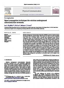
Figure 1.1: Simplified schematic of a typical borehole. Drill mud flows through the drill string and drill bit, transporting the cuttings out of the wellbore through the annulus. losses, environmental damages or personnel injuries are avoided. Due to the length of the wells, and the need for real-time data during drilling operations, the downhole pressure is not available for direct measurement, and would in addition be affected by disturbances. The need for a satisfying fit-for-purpose model for estimating the states is therefore present. Figure 1.1 illustrates a typical borehole placed down in the seabed. This is one of many applications where state estimation is a crucial part of the overall procedure and performance, where direct measurements are not available.

1.2

Derivation of more efficiently state estimation algorithms

Considering that an estimation scheme approximates the states in a system or process, it is obvious that the computational complexity increase with the size and complexity of the system. Thus, problems may arise when the number of states makes the computational complexity too extensive to calculate within a given time limit, i.e., in real-time operations as mentioned earlier. Due to limited resources in terms of hardware, simpler and more efficient models are 2

1.3. PROBLEM FORMULATION

required in order to meet the requirements of some processes. Some approaches for the derivation of simpler models are Finding similar, less complex, models Using models that are less complex, but still is similar enough to use in estimation of the states, so-called fit-for-purpose models, can reduce the computationally complexity. The disadvantage of this approach is that finding a less complex, yet similar to the true model, can be difficult. Finding an appropriate full model by using physical laws can be hard enough. Using model reduction By using existing techniques for model reduction, the existing full model can easily be reduced to a smaller model, and further used in the calculation for estimating the states. The advantage of this approach is that there exists a lot of techniques for model reduction, but it may, however, lead to some loss in information when projecting and reconstructing the full model.

The main difference between the two approaches is that the fit-for-purpose model requires prior knowledge about the process, while using model reduction can generally be used on any existing model (to some degree).

1.3

Problem formulation

The main advantage of reducing the complexity of the state estimation techniques is that the overall computational cost is reduced. However, the estimation result, when reducing the complexity, may be affected such that the error between the true and estimated states should be kept at a minimum. Achieving both of these criteria are highly beneficial, as nature consists of large nonlinear and complex systems, making the process of state estimation a very computationally expensive task. In state estimation theory, the most well-known state estimation algorithm is the Kalman Filter (KF), developed during a research supported by the U.S. Air Force Office of Scientific Research by [Kalman, 1960]. This algorithm exists both in a linear and nonlinear edition, making it suitable for most of the processes in nature. Similar approaches such as the Unscented Kalman Filter (UKF), [Julier et al., 2004] and the Ensemble Kalman Filter (EnKF), [Evensen, 1994] has also gained popularity since they were developed. Several less computational 3

1.4. PREVIOUS WORK

expensive variants of these also exists [Julier, 2003, Julier and Uhlmann, 2002, Quine, 2006]. In terms of model reduction, reduced order models can be derived by various methods. Some are for example truncating states, either from a unbalanced or balanced representation [Skogestad and Postlethwaite, 2005], or Proper Orthogonal Decomposition (POD), also known as Karhunen-Lo`eve decomposition [Lall et al., 2002], where each of the techniques have desirable properties depending on the system which is to be reduced. Using Galerkin projection [Lall et al., 2002], allows the projection of the full model to a reduced model, or reconstructing the full model from the reduced model, through similarity transforms. Thus, the technique makes it applicable to only use the reduced model in some parts of the state estimation. Specifically, the reduced model can be used in the covariance propagation in the Extended Kalman Filter (EKF) or calculation of the sigma points in the UKF, while using the full model for propagating the states or transforming the sigma points. This should lead to a improvement in the computational complexity for estimating the states of a given system, while hopefully giving a satisfying estimation result. This is the main motivation of this Masters study. Given a higher-order nonlinear process, find more efficient ways for state estimation through the use of EKF or UKF, which meets the following characteristics: the reduced model should have a substantially lower dimension than the full (original) model, the reduced model should keep all relevant dynamics, the new approach should retain a sufficient accuracy level, the new approach should be more efficient than the original model, and the new approach should have benefits over existing reduced approaches.

1.4

Previous work

In the literature regarding model reduction and nonlinear state estimation, it seems that most of the studies are based on using the reduced model for the entire estimation process. On the subject of reducing the computational effort, which in amongst other fields is important for image processing, [Burl, 1993] have shown how combining the EKF in estimation of a image reconstruction and 4

1.5. THESIS OUTLINE

velocity of objects, gives a large reduction in number of multiplication operations and vastly time savings on the inversion of matrices. The results of [Burl, 1993] also showed that given a known velocity, the image reconstruction was found to be close to the optimal result. A similar study on reducing computational cost by [Farrell and Ioannou, 2001], conducted on a forecast error system of a mid-latitude storm model, showed great approximation and performance using a reduced model. It was shown that the 400 Degrees of Freedom (DOF) model, where the dynamically relevant dimension is much smaller then the full state dimension, could be reduced to a 60 DOF model through balanced truncation, while giving a satisfying accurate approximation. Another interesting study for reducing the KF is a study on reducing the full system model without model reduction, which have been conducted with good results. According to [Simon, 2007], given that the transition matrix has some given form and is stable, it is shown that the computational effort was substantially decreased in contrast to using normal model reduction techniques. However, this specific method led to an increase in the estimation error and could not guarantee convergence and stability in the computation of the Kalman gain. In several studies regarding reduction of the computational cost in the EKF, leading up to the paper by [Evensen, 1994], Evensen showed that solving the Kolmogorov’s equation using Monte Carlo methods in forecast error statistics, is an alternative to solving the approximate error covariance equation. This technique, known as the EnKF, showed great performance compared to the EKF as there are no closure problem, with only a fraction of the computational load for reasonable accuracy.

1.5

Thesis outline

The thesis is organized as follows. Chapter 2 presents the relevant theory with respect to state estimation and model reduction. The mathematical outline and algorithms for the most common state estimation techniques are presented, alongside some more efficient derived variants. The most common techniques for model reduction will be presented, both for unbalanced and balanced model reduction, in addition to an overview of the implementations related to this thesis. Chapter 3 discuss the connection and use of state estimation algorithms in combination with the techniques from model reduction to reduce the bulk of 5

1.5. THESIS OUTLINE

complexity in the algorithms. The new, derived, approach is presented in full for both the EKF and UKF. Chapter 4 introduce the Partial Differential Equation (PDE) models used for illustration purposes in this thesis. The models are one and two dimensional heat conduction models, respectively, discretized by the Finite Volume Method, which is one of the most popular discretization techniques in Computational Fluid Dynamics (CFD) software. This chapter also discuss the strategy and approach of finding a reduced order basis corresponding to the full models through the use of POD. In Chapter 5, the hardware and software setup are presented. This involves the computer specifications, the experimental setup for the simulation, and the conditions imposed on the testing environment to ensure accurate and valid data. Chapter 6 represent and discuss the results from the simulation of the models. The algorithms are mainly obtained with POD as the model reduction technique, but balanced truncation by empirical Gramians is also considered. The simulations are conducted for different scenarios, inducing errors such as Gaussian white noise, and systematic and model errors. The data of the time complexity, estimation results and problems encountered with the simulations are discussed. Finally, in Chapter 7, conclusions and recommendations for future research are given.

6

2

Background material 2.1 State estimation 2.2 Model reduction

2.3 Implementation

This chapter introduce the tools and techniques that will be used in the subsequent chapters to develop reduced-order models and perform state estimation. The tools and techniques are either described in full, or summarized by the outline of the algorithm/technique.

2.1

State estimation

State estimation is the technique of approximating or predicting the states in a process based on measurements from the process. In engineering, the information gathered from state estimation may be of interest of their own, or even necessary for example in control purposes. The problem statement, alongside different techniques of state estimation are presented.

2.1.1

Problem statement

The problem statement of state estimation is given as follows. Assume that a real system can be represented by the differential equation ˙ x(t) = f (x(t), u(t)) + w(t),

(2.1a)

y(t) = h (x(t), u(t)) + v(t),

(2.1b)

where x ∈ Rn is the state vector, u ∈ Rp is the p inputs to the system, w ∈ Rn and v ∈ Rm are the process and measurement zero-mean Gaussian white noise vectors added to the system, and y ∈ Rm the m measurements of the system. The objective is to estimate the real states, ˆ˙ (t) = f (ˆ x x(t), u(t)) , ˆ (t) = h (ˆ y x(t), u(t)) , 7

2.1. STATE ESTIMATION

based on measurements from the real system, such that the estimated states are ˆ ' x. similar or equal to the true states, i.e., x Since this thesis is concerned with discrete time systems, the discrete-time versions of the algorithms are presented.

2.1.2

Linear systems

Discrete linear time-invariant systems, or nonlinear systems that are linearized within a small region, are generally described as xk = Ak−1 xk−1 + Bk−1 uk−1 + wk−1 ,

(2.3a)

yk = Ck xk + Dk uk + vk ,

(2.3b)

where the set of equations represents the internal description of the system. Linear systems have the advantage that they are much simpler than their nonlinear counterpart, making one of the most known state estimation techniques apply to linear systems. The Kalman Filter [Kalman, 1960] presents a method for solving the Wiener problem and show how estimates of the discretized state vector xk , based on the knowledge of the system and the measurement vector yk , at time tk , can be obtained. This section will present the Kalman Filters recursive equations, which makes up the procedure of estimating the states. Suppose that the objective is to estimate the linear state-space system (2.3). Given that the data up to and including time tk can be obtained, an a posteriori estimate of the state can be formed. The a posteriori estimate is the estimate after the measurement yk is taken into account and is given as ˆ+ x k = E [xk |y1 , y2 , . . . , yk ] , where the operator E [·] denotes the expected value of (·). Based on the measurements and previous states, the goal is to approximate the states such that the error between the estimated and true states are minimized, i.e., ∆

ˆ− e− k, k = xk − x with the associated covariance matrix given as − − T P− k = E ek (ek ) T ˆ− ˆ− = E (xk − x . k )(xk − x k) 8

(2.4)


The covariance matrices related to the process and measurement noise vectors in (2.3) are given as E wk wT i =

E vk vT i =

E wk vT i = 0,

Qk , 0,

i=k , i 6= k

(2.5a)

Rk , 0,

i=k , i 6= k

(2.5b)

∀ i, k,

(2.5c)

where it is given that the process and measurement noise vectors are uncorrelated. Given the terms above, the approach of the algorithm is outlined next. Approach The initialization of the estimation process starts with the a posteriori estimate of the initial state vector x0 . Since no measurements are available initially, it is reasonable to set this as the expected value of the initial states, given as ˆ+ x 0 = E(x0 ).

(2.6)

Further, as the mean of the state propagates with time, ¯ k = Ak−1 x ¯ k−1 + Bk−1 uk−1 , x ˆ , is the a priori estimate, known as the time update equation for the estimate x given in general form as ˆ− ˆ+ x k = Ak−1 x k−1 + Bk−1 uk−1 . The covariance of the state estimation error, denoted by P, is initialized by computing the a posteriori estimate. If one happen to know the initial states + (perfectly), one can set P+ 0 = 0, or P0 = ∞I if no prior knowledge of the initial states are known. In general, the covariance of the state estimation error is computed by T ˆ+ ˆ+ P+ . 0 )(x − x 0) k = E (x − x

(2.7)

Finally, the measurement-update equations for the gain, state estimate and the covariance of the state estimation error are necessary to introduce. These are 9


ˆ− Enter prior estimate x 0 and its error covariance P− 0 Compute Kalman gain: −1 T − T Kk = P− k Ck Ck Pk Ck + Rk

y0 , y1 , . . .

Project ahead: ˆ− ˆk x k+1 = Ak x = Ak Pk ATk + Qk

Update estimate with measurement yk : ˆk = x ˆ− ˆ− x k + Kk (yk − Ck x k)

P− k+1

ˆ0, x ˆ1, . . . x Compute error covariance for updated estimate: T T Pk = (I − Kk Ck )P− k (I − Kk Ck ) + Kk Rk Kk

Figure 2.1: The illustration of the Kalman Filter iteration loop (adapted from [Brown and Hwang, 1996]) show the iterative process in the algorithm. Given − ˆ− an initial a priori state estimate x 0 and belonging error covariance matrix P0 , the algorithm computes the Kalman gain and updates the estimate based on the current measurements. The error covariance is then calculated before the a posteriori estimate for the states and the covariance matrix are projected ahead. given by −1 T − T Kk = P− k Ck Ck Pk Ck + Rk T −1 = P+ k Ck Rk ,

ˆ+ x k + Pk

=

ˆ− x k

+ Kk yk −

ˆ− Ck x k

10

(2.8b) (2.8c)

T

T = (I − Kk Ck ) P− k (I − Kk Ck ) + Kk Rk Kk h i −1 −1 −1 = P− + CT k Rk Ck k

= (I − Kk Ck ) P− k,

(2.8a)

(2.8d) (2.8e) (2.8f)


where the matrix Kk is called the Kalman gain, which minimizes the meansquare estimation error. Note that there are three expressions for the covariance matrix of the state estimation error. This is due to that the first equation (2.8d) is valid for any gain, while the others are only valid for the optimal gain condition. To summarize the steps of the algorithm, a graphical illustration of the iteration process is given in Figure 2.1.

2.1.3

Nonlinear systems

Processes are rarely (as good as never) linear, and the linearization of nonlinear systems are not always possible, making state estimation techniques for nonlinear systems necessary. There exists several approaches for nonlinear state estimation with different properties, where some of the most known will be presented in the subsequent sections.

The Extended Kalman Filter The EKF is an nonlinear extension to the original Kalman Filter where the main difference is the linearization of the nonlinear system around the state estimate, making the outline of the algorithms very similar. Thus, when using the EKF to estimate a linear system, the approach of the EKF will be identical to the linear Kalman Filter. The approach of the algorithm is as follows.

Approach As shown in [Simon, 2006b], the discretized nonlinear process of (2.1) is given by xk = fk−1 (xk−1 , uk−1 ) + wk−1 ,

(2.9a)

yk = hk (xk , uk ) + vk ,

(2.9b)

where the covariance matrices for the vectors vk , wk are the same as in the linear case, given by Equation (2.5). In addition, the initialization of the a posteriori estimate and process covariance is equal to the linear case as given in Equation (2.6) and (2.7), respectively. The necessary linearizations for calculating the time update of the a priori state estimates and the estimation error covariance 11


matrix, are obtained by computing the Jacobians ∂fk−1 , Fk−1 = ∂x xˆ + k−1 ∂fk−1 Lk−1 = , ∂w xˆ +

(2.10a) (2.10b)

k−1

which makes it possible to calculate the covariance update and states + T T P− k = Fk−1 Pk−1 Fk−1 + Lk−1 Qk−1 Lk−1 ,

(2.11a)

ˆ− x k

(2.11b)

= fk−1 (xk−1 , uk−1 ) .

The necessary Jacobians for calculating the Kalman gain, state estimates and a posteriori estimation-error covariance matrix are given by ∂hk Hk = , (2.12a) ∂x xˆ − k ∂hk Mk = , (2.12b) ∂v xˆ − k

(2.12c)

leading up to the final calculation. The prediction step, given as −1 T T − T Kk = P− , k Hk Hk Pk Hk + Mk Rk Mk ˆ+ ˆ− ˆ− x , k =x k + Kk yk − hk x k , uk

P+ k

= (I −

K k H k ) P− k.

(2.13a) (2.13b) (2.13c)

which completes the presentation of the EKF with the necessary calculations for estimating a nonlinear system. It should be noted that [Simon, 2006b] use a square-root formulation of the EKF, which gives better numerical stability and precision of the covariance matrix. Ensemble Kalman Filter The EnKF by [Evensen, 1994] is a state estimation algorithm based on forecasting the error statistics using Monte Carlo methods. By creating an ensemble of state estimates, statistical samples used in forecasting and analysis, this can be 12


used to estimate a classical Kalman gain and predict error statistics. The EnKF is considered a highly efficient nonlinear state estimator, and will in this thesis be used for comparison reasons. The EnKF has the advantages that it is suited for systems with a large number of states, and that the covariance matrix is replaced by a sample covariance matrix computed from the ensemble, i.e., using statistics for obtaining the covariance matrix. EnKF Algorithm The outline of the EnKF presented in this thesis is based on the article by [Gillijns et al., 2006], as given below in Algorithm 1. The reader is referred to [Evensen, 1994, Burgers and et al., 1998] for a more detailed mathematical description of the theory and algorithm. Algorithm 1: Ensemble Kalman Filter Input : A priori ensemble analysis estimate xa0i , i = 1, . . . , q. Output: Analysis ensemble estimate xaki , i = 1, . . . , q, analysis mean ¯ aki , i = 1, . . . , q x 1 2 3 4 5 6

7 8 9

/* Forecast step

*/

for k ← 0 to n do i xfk+1 = f (xaki , uk ) + wik , i = 1, . . . , q; P i ¯ fk+1 = 1q qi=1 xfk+1 x ; h i fq 1 ¯ fk+1 , . . . , xk+1 ¯ fk+1 ; −x −x Efk = xfk+1 h i ¯ fk ; ¯ fk , . . . , yk fq − y Efyk = yfk1 − y T f T f f 1 ˆ ˆ f = 1 Ef Ef = , P ; E E P yy k y y y xyk q−1 q−1 k k k k

*/

/* Analysis step f −1 ˆk = P ˆf ˆ K ; xyk Pyyk ai fi ˆ k yk + v i − h(xfi , ui ) , i = 1, . . . , q; xk = xk + K k k k P ¯ ak = 1q qi=1 xaki ; x

It should be noted that the index k refers to the time index, n the total number of samples, q the total number of ensembles, and wik , v ik , i = 1, . . . , q, are zero-mean random variables with a normal distribution and covariance Rk , Qk , respectively. 13


Unscented Kalman Filter To avoid the limitations of the EKF with the linearization of the state equations, an unscented transformation and state estimation algorithm, were developed by [Julier et al., 2004] to propagate the mean and covariance information through nonlinear transformations. This approach, called the UKF, approximates a probability distribution, rather than approximating an arbitrary nonlinear function, reducing the errors which occurs in the EKF.

Approach Following the approach presented in [Simon, 2006b], given a discretetime nonlinear system (2.9) with its belonging covariance matrices (2.5), the UKF is initialized similar to the approach of the KF. Due to no initial available measurements, it is reasonable to set the a posteriori state and covariance as given in Equation (2.6) and (2.7), respectively, with respect to the initial state x0 . The procedure starts by obtaining the time update equations through an unscented transformation to estimate the true mean and covariance of a known nonlinear function by a set of deterministic vectors, as illustrated in Figure 2.2. (i) ˆ k−1 are, since the best guess of The vectors, called sigma points, denoted by x + + ˆ k and Pk−1 , chosen as the mean and covariance of xk are x (i)

ˆ k−1 = x ˆ+ ˜ (i) , x k−1 + x q T + (i) ˜ = x nPk−1 ,

i = 1, . . . , 2n,

(2.14a)

i = 1, . . . , n,

(2.14b)

i = 1, . . . , n,

(2.14c)

i

˜ (n+i) = − x

T q nP+ , k−1 i

q T q + nP+ is the matrix square root such that nP nP+ k−1 k−1 k−1 = q q nP+ nP+ is the ith row of nP+ k−1 , and k−1 k−1 (see Appendix B.2 for where

q

i

details of the matrix square root). The sigma points are then transformed into (i) ˆ k by using the state equation the vectors x (i) (i) ˆk = f x ˆ k−1 , uk + wk , x 14

(2.15)


Sigma points

Transformed sigma points UT covariance

Unscented Transformation

UT mean

Covariance

Mean

True mean

True covariance

Figure 2.2: Illustration of the unscented transformation in the UKF, which approximates the covariance and mean of the nonlinear system. The left show the true mean and covariance of the system with a deterministically chosen set of points, while the right show the applied transformation with its corresponding estimated covariance and mean.

which are further used to obtain the a priori state estimate and error covariance

2n

ˆ− x k =

1 X (i) ˆ , x 2n i=1 k

(2.16a)

T 1 X (i) (i) ˆk − x ˆ− ˆk − x ˆ− x x + Qk−1 . k k 2n i=1 2n

P− k =

(2.16b)

Similar to the calculation of the time update equations, as the current best guess − ˆ− for the mean and covariance of xk are x k and Pk , the sigma points are chosen as (i)

ˆk = x ˆ− ˜ (i) , x k−1 + x T q − (i) ˜ = x nPk ,

i = 1, . . . , 2n,

(2.17a)

i = 1, . . . , n,

(2.17b)

i = 1, . . . , n.

(2.17c)

i

˜ (n+i) = − x

q T nP− , k i

15


(i)

ˆ k by The sigma points are then transformed into predicted measurements y using the state measurement equation, i.e., (i) (i) ˆk = h x ˆ k , uk , y (2.18) making it possible to obtain the predicted measurement and its belong covariance matrix by 2n

ˆk = y

1 X (i) ˆ , y 2n i=1 k

(2.19a)

T 1 X (i) (i) ˆk − y ˆk y ˆk − y ˆk y + Rk . 2n i=1 2n

Py =

(2.19b)

It is then necessary to calculate the estimate of the cross covariance between ˆ− ˆk, x k and y 2n T 1 X (i) (i) ˆk − x ˆ− ˆ ˆ x y − y , (2.20) Pxy = k k k 2n i=1

which makes the measurement update of the state estimate, using the normal Kalman Filter equations, to be calculated by Kk = Pxy P−1 y , ˆ+ x k P+ k

= =

ˆ− ˆk) , x k + Kk (yk − y − T Pk − Kk Py Kk .

(2.21a) (2.21b) (2.21c)

To make the UKF algorithm more rigorous, as it in this approach treats the noise as additives in Equation (2.16) and (2.19), respectively, an augmented version of h the algorithm i exist. This involves augmenting the state T a T T vector as xk = x ˆ k vk wk ∈ Rna , na = nx + nv + nw , and using the augmented vector throughout the algorithm. This approach is described in full in [Julier et al., 2004, Wan and van der Merwe, 2000]. Reduced sigma point filters Due to the computational complexity in the calculation of the sigma points in the UKF, [Julier and Uhlmann, 2002] proved that for an n-dimensional system, only n+1 sigma points (minimal skew sigma points) are required to capture the mean 16


and covariance. This could potentially be a unstable and unreliable algorithm as the set of sigma points can lead to numerical problems. However, based on the minimal skew sigma points, [Julier, 2003] describes a better-behaved sigma point selection strategy, known as the Spherical-Simplex Unscented Kalman Filter (SSUKF), which requires only n + 2 sigma points. This approach defines a simplex of points that lie on a hypersphere. These points, known as spherical simplex points, lie on the origin or on a hypersphere centered at the origin, √ making the points lie in a radius proportional to n, and the weights applied proportional to 1/n. The spherical simplex points are then calculated using the following criterion p ¯ + Px Z i , Xi = x i = 0, . . . , n + 1 √ where Px is a matrix square root of Px and Z i is the ith column of the spherical sigma point matrix calculated by 1. Choose 0 ≤ W0 ≤ 1. 2. Choose weight sequence: Wi =

1 − W0 , n+1

i = 1, . . . , n + 1

3. Initialize vector sequence as: Z 10 = [0] ,

1 Z 11 = − √ , 2W1

4. Expand vector sequence for j = 2, . . . , n  j−1 Z0       # " 0 j−1    Zi Z ji = −√ 1  j(j+1)W1  " #    0  j−1    √ j

1 Z 12 = √ 2W1

according to for i = 0 for i = 1, . . . , j for i = j + 1

j(j+1)W1

The spherical sigma points are then incorporated into the UKF, with some minor differences from the original algorithm. The reader is referred to the original article for further details. 17


Derivative-free Extended Kalman Filter The Derivative-Free Extended Kalman Filter (DFEKF) by [Quine, 2006] is based on the propagation of a minimal ensemble set of n + 1 state vectors, making it computationally advantageous. It is similar to the EKF as it propagates only the first two moments of any state distribution, and can be shown to be equivalent to the EKF in a limiting case (see [Quine, 2006] for details). The outline of the state estimation algorithm is summarized in pseudo-code below. 1. Prediction stage ˆ (a) Form a set of vectors by using previous or initial state estimates x and covariance Px p ∆xi ˆ+ , i = 1, . . . , n, where {∆x1 . . . ∆xn } ≡ nPx Xi = x α

ˆ by (b) Predict the value of X i , x

X i = f (X i ) , i = 1, . . . , n,

ˆ = f (ˆ x x)

and project the state covariance n α2 X ˆ ) (X i − x ˆ )T + Q. (X i − x Px = n i=1

(c) Form a set of vectors for projection ˆ+ Yi = x

∆yi , i = 1, . . . , n, α

where {∆y1 . . . ∆yn } ≡

ˆ by (d) Predict the observation value of Y i , x Y i = h (Y i ) , i = 1, . . . , n,

ˆ = h (ˆ y x) .

2. Update stage (e) Calculate the covariances Pxy , Pyy by Pxy = Pyy

n α2 X ˆ ) (Y i − y ˆ )T , (X i − x n i=1

n α2 X ˆ ) (Y i − y ˆ )T + R. = (Y i − y n i=1

18

p

nPx

2.2. MODEL REDUCTION

(f) Form weight matrix and update state and covariance estimates by K = Pxy P−1 yy , ˆ=x ˆ + K (y − y ˆ) , x

Px = Px − KPT xy .

(g) Repeat recursively to generate time-evolving estimates of state and covariance. The parameter α is a scaling parameter, which is discussed in full in [Quine, 2006].

2.2

Model reduction

This section presents the theory associated with model reduction, a technique of reducing the number of states in large-scale models to simpler models with similar dynamics.

2.2.1

Problem statement

The problem statement of model reduction is given as follows by [Hovland, 2008, Lall et al., 2002]. Given a system represented by the nonlinear differential equations (2.1), the objective is to find a reduced system represented by the differential equations x˙ r (t) = fr (xr (t), u(t)) , yr (t) = hr (xr (t), u(t)) , where xr ∈ Rr and yr ∈ Rm such that r < n, where n is the total number of states in the original system (2.1), while having a “small” approximation error, numerical stability and computationally efficiency. A typical measure of the error can according to [Skogestad and Postlethwaite, 2005] be given as kG(s) − Gr (s)k∞ , where G(s), Gr (s) are the transfer functions of the full and reduced system, respectively, and the infinity norm is either a Hankel (H∞ ) or L∞ norm. 19


2.2.2

Projection

Projection is a mathematical approach of mapping a set into a subset, such as transforming points or vectors from one plane (or dimension) to another plane [Antoulas, 2005]. Consider a three-dimensional Euclidian vector x(t) as given in Figure 2.3, where the vector is projected down onto the subspace S ⊆ R2 by a projection operator Φr . The projection operator represent the relationship between the two-dimensional vector xr (t) and the original three-dimensional vector x(t).

y

z

x(t)

x

S

xr (t)

Figure 2.3: Illustration (adapted from [Farhat, 2013]) of orthogonal projection, where the three-dimensional vector x(t) is projected onto a twodimensional subspace S at time t. In terms of model reduction, projection is more commonly known as Galerkin projection [Lall et al., 2002, Hovland, 2008], where the general idea of projectionbased reduction is to search for a subspace spanned by a projection matrix Φ = {φ1 , φ2 , . . . , φn } containing the eigenvectors corresponding to the largest eigenvalues of the system. If the eigenvalues are ordered in increasing or decreasing order, the irrelevant eigenvalues can be omitted such that the only relevant information from the system are kept. For a general system (2.1), it is assumed that the state vector x can be approximated by a linear combination of r basis vectors x ' Φr xr 20


where xr ∈ Rr is the reduced state and the reduced projection matrix Φr ∈ Rn×r contains the r basis vectors φ1 , φ2 , . . . , φr so that ΦT r Φr = Ir . This leads to that the general nonlinear reduced system of (2.1) is given by x˙ r (t) = ΦT r fr (Φr xr (t), u(t)) , yr (t) = hr (Φr xr (t), u(t)) . For the linear discrete case, the projected reduced model of (2.3) becomes x˙ r,k = Ar xr,k−1 + Br uk−1 , yr,k = Cr xr,k + Dr uk , where the reduced system matrices are projected as Ar = ΦT r AΦr ,

(2.25a)

ΦT r B,

(2.25b)

Cr = CΦr ,

(2.25c)

Dr = D.

(2.25d)

Br =

There exist several methods for obtaining the projection matrix Φ, where some of the methods will be presented in the subsequent sections.

2.2.3

Proper Orthogonal Decomposition

POD, which according to [Holmes et al., 1996, Hovland, 2008] is also known as principal component analysis, Karhunen-Lo´eve expansion and Singular Value Decomposition (SVD), is a method of least-squares approximation. It was initially developed by [Lumley, 1967] for use in the field of fluid mechanics to study turbulent flows, but has over the years become one of the most popular methods of nonlinear model reduction. Theory [Astrid et al., 2002, Lall et al., 2002, Hovland, 2008] states that POD provides a basis for the compact representation of an ensemble of data, such as a finite number of N samples x(tk ), k = 1, . . . , N from the system (2.1) in a matrix of snapshots Tsnap . By characterizing a subspace S ⊂ Rn by the projection operator Φr , the objective is to find the POD basis that minimize the error 21


between the original snapshots and their representation in the reduced space, i.e., the total squared distance of the points from the r-plane min H(Φr ) = Φr

N X

k=1

˜ (tk )k22 , kx(tk ) − x

(2.26)

˜ (tk ) = Φr ΦT where x r x(tk ) and r is the order of approximation. The minimizing solution Φr can be found by the set of left singular vectors of Tspan , Tspan = ΦΣΨT ,

(2.27)

where Φ contains the orthogonal basis vectors and Σ = diag(σ1 , . . . , σs ) contains the associated singular values. The r most significant basis functions are associated with the r largest singular values σi , i = 1, . . . , r. If the singular values σi has a significant drop in magnitude between i = r, r + 1, a reduced-order model may be constructed by using the projection operator Φr , corresponding to the r first columns of Φ. When projecting onto a subspace S, the energy conservation in the model is of concern. Particularly, how close the approximation of data provided by an r-dimensional subspace is important and can be measured by comparing the fraction of the total ‘energy’ Pr

P = Pi=1 N i=1

σi σi

,

(2.28)

where the goal is to choose r such that the energy in the subspace is approximately the same as the full space, i.e., P ' 1, while keeping r sufficiently small. Keep in mind that the validity of approximations is defined by the correlation matrix Tspan , and is limited to how well this represent the dynamics of the system. In addition, if the system is unstable, the corresponding responses may make an approximation by orthonormal basis impossible. POD Algorithm From the previous section, it comes clear for the perceptive reader that the calculation of Equation (2.27) is simply the SVD of the snapshot matrix Tspan . The outline of the POD algorithm is restated from [Hovland, 2008] below in Algorithm 2. 22


Algorithm 2: Proper Orthogonal Decomposition Input : Matrix of N snapshots, Tsnap = {x(1) , x(2) , . . . , x(N ) }. Output: Matrix of the r most significant basis vectors, Φr 1

Compute the SVD of the snapshot matrix Tspan Tspan = ΦΣΨT

2

Extract the r most significant basis vectors Φr based on the singular values σi of Tsnap

3

Project the state equations onto the reduced basis as described in Section 2.2.2.

2.2.4

Model reduction by balanced truncation

Balanced truncation is merely the method of truncating a balanced system. A balanced system, or balanced realization, is given by [Green and Limebeer, 1994] as the approach of balancing the past input and output “energy” in the system. More generally, the controllability and observability Gramians are equal and diagonal. Truncating a system corresponds to ordering the states based on the information they contain, and removing the states which contain little or irrelevant information. Thus, the truncated (reduced) system share approximately the same dynamics as the full system.

Linear systems A general linear state-space system is given on the form presented in Equation (2.3), where x, u and y have the same dimensions as the vectors given in Equation (2.1). A balanced realization of a linear system (2.3), is an asymptotically stable minimal realization in which the controllability and observability Gramians are equal and diagonal. According to [Green and Limebeer, 1994], a balanced realization is most commonly defined as

23


Definition 2.2.1. A realization (A, B, C) is balanced if A is asymptotically stable and AΣ + ΣAT + BBT = 0, AT Σ + ΣA + CT C = 0, in which  σ1 Ir1  Σ= 0 0

0 .. 0



0 .

 0 , σ m I rm

σi 6= σj , i 6= j and σi > 0 ∀i.

Note that n = r1 + . . . + rm is the size (called the McMillan degree) of C(sI − A)−1 B and that ri is the multiplicity of σi . We say that the realization is an ordered balanced realization if, in addition, σ1 > σ2 > . . . > σm > 0. To be able to validate the controllability and observability of a system, the associated Gramians needs to be calculated. The definitions of the controllability and observability Gramian are defined in [Green and Limebeer, 1994] as given below. Definition 2.2.2. The dynamical system x˙ = Ax + Bu, or the pair (A, B), is state controllable if and only if the Gramian matrix ∆

Wc (t) =

Z

T

eAτ BBT eA

T

τ

dτ

0

has full rank for any t > 0. Equivalently, for a stable system, the pair (A, B) is state controllable if and only if the controllability Gramian Z ∞ T ∆ Oc = eAτ BBT eA τ dτ 0

is positive definite. Oc may also be obtained as the solution to the Lyapunov equation AOc + Oc AT = −BBT . 24


Definition 2.2.3. The dynamical system x˙ = Ax + Bu, y = Cx + Du or the pair (A, C), is state observable if and only if the observability Gramian Z ∞ T ∆ Oo = eA τ CT CeAτ dτ 0

has full rank. Oo may also be obtained as the solution to the Lyapunov equation AOo + Oo AT = −CT C. Using the theory above for obtaining a balanced realization, and assuming that the system (2.3) has been balanced, the system can be partitioned as x1,k = A11 x1,k−1 + A12 x2,k−1 + B1 uk−1 , x2,k = A21 x1,k−1 + A22 x2,k−1 + B2 uk−1 , yk = C1 x1,k + C2 x2,k + Duk , where x1 ∈ Rn−r , x2 ∈ Rr . In addition, assuming that the r states associated with x2 contains no relevant dynamics, the states can be truncated making the reduced system share approximately the same amount of information as the full system. Similar approaches to model reduction using projection through balanced truncation for the linear case exists, for example by using the method of balanced truncation by [Laub et al., 1987]. Nonlinear systems The theory of the Gramians from Definition 2.2.2-2.2.3 is not applicable for nonlinear systems, and since nonlinear energy functions are difficult to obtain, [Lall et al., 2002, Hahn and Edgar, 2002b] presents the method of using empirical Gramians in model reduction for control purposes. This is considered an extension to balancing linear systems, as described in the previous section. The approach involves computing controllability and observability covariance matrices, where a transformation can be used with a Galerkin projection to achieve a nonlinear balanced form. The balanced equations can then be reduced by truncating the states corresponding to small Hankel singular values. 25


Theory The empirical Gramians have to be determined from data, either generated experimentally or by simulation, where the data should be collected within the region where the process is to be controlled. To define the empirical Gramians for a nonlinear system (2.1), the following sets are required: n o T n = T1 , . . . , Tj ; Ti ∈ Rn×n , TT (2.30a) i Ti = I, i = 1, . . . , j M = {c1 , . . . , cs ; ci ∈ R, ci > 0, i = 1, . . . , s} n

n

E = {υ 1 , . . . , υ n ; standard unit vectors in R }

(2.30b) (2.30c)

where j is the number of matrices for perturbation directions, s the number of different perturbation sizes for each direction and n the number of states of the full order system. The sets T and E are used to determine the input directions, and M specify the size of the inputs and states we are interested in, where the dynamics should evolve in a region close to the operating area. An initial reasonable choice of the sets (2.30) are T = [I, − I], E = I, while the set M can be chosen arbitrarily according to the desired perturbation magnitude. The choice of the set T corresponds to using both positive and negative inputs (or initial states) on each input separately. The main advantage of the following approach is that it requires only the solution of the standard linear matrix eigenvalue problem, where the empirical Gramians are restated from [Hahn and Edgar, 2002a] in Definition 2.2.4 and 2.2.5 below. Definition 2.2.4. Let T p , E p and M be given sets as described above, where p is the number of inputs. The discrete empirical controllability Gramian is defined by q j X p s X X 1 X ilm ∆ Θk ∆tk Wec = jsc2m k=0 l=1 m=1 i=1 ilm T ilm where Θilm ∈ Rn×n is given by Θilm = xilm − xilm xk − xilm , xk is k k ss ss k the state of the nonlinear system (2.1) at time step k corresponding to the input uk = cm Tl υ i δi + uss,0 1 , and xilm ss is the desired system trajectory. Definition 2.2.5. Let T n , E n and M be given sets as described above, where n is the number of states. The discrete empirical observability Gramian is defined by j X q s X 1 X ∆ T Weo = Tl Ψlm k Tl ∆tk 2 jsc m m=1 l=1

1δ

k=0

denotes Dirac’s delta function.

26

2.2. MODEL REDUCTION T ilm ilm n×n ilm where Ψlm , yk is is given by Ψlm yk − yilm − yilm k ∈ R ss k ij = yk ss the output of the nonlinear system (2.1) corresponding to the initial condition x0 = cm Tl υ i + xss , and yilm ss is the steady state the system will reach after this perturbation. From the empirical Gramians it is possible to obtain a balanced realization through the subspace approach by [Lall et al., 2002], or by the algorithm given in [Hahn and Edgar, 2002a]. The approach by [Lall et al., 2002] is developed for control purposes, where the computation for balancing the empirical Gramians is as follows. Apply the Cholesky decomposition (see Appendix B.2) to Wec so that Wec = LLT , where L is a lower triangular matrix with non-negative diagonal entries. Then let UΣ2 VT be the SVD of LT Weo L, and 1

Φ = Σ 2 VT L−1 be the change of coordinates such that the system is balanced. The states with small Hankel singular values σi are then truncated. If the states are ordered according to decreasing singular values, this is equivalent to applying a Galerkin projection where the r most significant states are kept. The projection can easily be performed by introducing the “identity” vector Ig = [Ir 0], which results in the following balanced reduced system T ˜ k = Ig Φr fk−1 Φ−1 ˜ k−1 , uk−1 , x r Ig x T ˜ yk = hk Φ−1 I x , u . k k r g

It should be mentioned that [Hahn and Edgar, 2002b] shows that this approach is limited to control-affine systems, requiring modifications when the systems steady-state is different from zero. However, the approach by [Hahn and Edgar, 2002a] is limited to stable nonlinear systems, and due to quite intricate computations, the reader is asked to refer to the original paper for details.

27


2.2.5

Balanced Proper Orthogonal Decomposition

The balanced POD by [Rowley, 2005] obtains an approximation to balanced truncation that is computationally effective for large systems. Algorithm 3: Balanced Proper Orthogonal Decomposition 1

2

Integrate solutions x1 (t), . . . , xn (t) of the system x˙ = Ax, with initial conditions xk (0) = bk , where bk denotes the k-th column of the B matrix in the system (2.3). Compute POD modes φk of the dataset {Cx1 (t), . . . , Cxn (t)}, and choose a projection rank r such that the error kG − Pr Gk22 =

3

4

p X

λj

j=r+1

where G is the impulse response matrix, Pr is an orthogonal projection with rank r and p is the number of outputs, is acceptable. Integrate solutions z1 (t), . . . , zr (t) of the adjoint system z˙ = AT z, with initial conditions zk (0) = CT φk . Form the data matrices X and Y for the primal and dual solutions as h p p p p i X = x1 (t1 ) δ1 . . . x1 (tm ) δm . . . xn (t1 ) δ1 . . . xn (tm ) δm ,

5

where δj are quadrature coefficients. Compute the SVD of YT X Y X = UΣV = U1 T

T

Σ1 U2 0

0 VT 1 , 0 VT 2

and the balanced POD modes are given by −1

T1 = XV1 Σ1 2 , −1

T S1 = Σ1 2 UT 1Y .

The features of this technique are a combination of the features for balanced 28


realization and POD, making further elaboration unnecessary. The drawback of balanced POD is that it requires the dual system, which does not exist in nonlinear settings. However, this can be solved by linearizing the system and forming the dual, or by the method of empirical Gramians as described earlier. The procedure is summarized in Algorithm 3.

2.2.6

Goal-oriented model-constrained reduction

Goal-oriented model-constrained reduction is, in contrast to the previously presented techniques, a optimization problem proposed by [Bui-Thanh et al., 2007], which has the objective to find an optimal rth order basis Φr and corresponding reduced states xr that minimize a criteria similar to (2.26) in the POD. Consider a finite set with I different instances of the system (2.1), where the corresponding reduced-order system is of the form (2.2), the optimization problem on the interval (0, tf ) is given as I

1X min G = Φr ,xr 2

k=1

Z

tf

0

yk − ykr +

T

yk − yr k

dt

n n 2 β X 2 β X T φ + φ 1 − φT φ j j 2 j=1 2 i,j=1 i j

k k x˙ kr = ΦT r f r Φr x r , u k xkr0 = ΦT r x0 , ykr = hr Φr xkr , uk ,

subject to

(2.32a)

i6=j

,

k = 1, . . . , I,

(2.32b)

k = 1, . . . , I,

(2.32d)

k = 1, . . . , I,

(2.32c)

where β is a regularization parameter penalizing the deviation of the basis vectors from an orthonormal set, and x0 is the initial states. If the relationship between the outputs and states are linear, the objective function is given as I

1X G= 2

k=1

Z

0

tf

ˆk xk − x

T

n n 2 β X 2 β X ˆ k dt+ Hk xk − x 1 − φT + φT , j φj i φj 2 j=1 2 i,j=1 i6=j

T where Hk = Ck Ck is considered a weighting matrix defining the relevant

states to the specified output. The optimization problem (2.32) minimizes the output error, whereas the POD cost is related to minimizing the error over the 29

2.3. DIFFERENTIATION

entire state domain, making it more suitable for output-feedback implementation. However, by altering the minimizing criteria, for example to the largest degree of observability or minimizing the error in a specific state, the approach could potentially provide a better basis than the POD. Solving the optimization problem will in general be more computationally expensive than using the POD. The cost of solving the offline optimization problem should therefore be taken into consideration when choosing the procedure for obtaining the basis Φr .

2.3

Differentiation

In order to be able to perform the linearization, the calculation of the Jacobians, in the EKF, a differentiation technique is required. The choice for this thesis, due to its simplicity is a simple difference quotient. There exist many other techniques such as automatic and symbolic differentiation that are more numerical stable, but many of the other techniques are more computationally expensive.

2.3.1

Difference quotient

The most basic and simple numerical differentiation scheme is the difference quotient computation, which has the objective to add a small step length to approximate the next function value. Derived from Taylors theorem, the difference quotient is given by [Hass et al., 2011] as f (¯ x + α) − f (¯ x) + O(α), α→0 α

∇f (¯ x) = lim

α 6= 0

where α is a small positive scalar, x ¯ a column vector and O(α) is the error, provided that this limit exists. The notation O(α) should be read ‘big oh of α’ and indicates the upper limit of the error, which behaves linearly. The advantage of the difference quotient is that it only needs a valid function, but has the disadvantage that the accuracy is highly dependent on the value of α. The choice of α is somewhat of a paradox. A small value of α can reduce the number of significant figures, while if α is not small enough, truncation errors may become significant. 30

2.4. IMPLEMENTATION

2.4

Implementation

This section will summarize which algorithms and techniques that are actually implemented during the work related to the thesis. First, all of the state estimation algorithms are implemented according to the theory presented. The implementation of the algorithms are only assumed to be valid, as it is difficult to make satisfying tests which validate the state estimation algorithms sufficiently. Most of the model reduction techniques are implemented, but only the POD and the balanced truncation by [Lall et al., 2002] are actually used in this thesis. The two used implementations of the model reduction techniques are tested through “textbook examples” from their respective references or similar books/journals. Table 2.1 gives an overview of which methods from this chapter that are implemented and if they are validated. Table 2.1: Overview of the different techniques and methods from the background theory that are implemented and/or validated. Description

Implemented?

Validated?

EKF UKF EnKF SSUKF DFEKF

Yes Yes Yes Yes Yes

No No No No No

POD Balanced truncation, Lall Balanced truncation, Hahn Balanced POD Goal-oriented POD

Yes Yes

Yes Yes

Yes♠

No

Yes♠ No

No No

Yes

Yes

Difference quotient ♠

Implemented, but not used in this thesis.

31

3

Efficiency improvement in state estimation 3.1 Introduction 3.2 Projections

3.1

3.3 Extended Kalman Filter 3.4 Unscented Kalman Filter

Introduction

The complexity of state estimation, as discussed initially in the introduction, increase with the size and complexity of a system. Nevertheless, and regardless of the objective, a high computational complexity is never preferable, which in the context of this thesis, leads to seek for more efficient state estimation algorithms. From the previous work presented in Chapter 1, on the subject of efficiency improvement, the common approach is to use the reduced model throughout the entire state estimation algorithms. This includes using reduced models in both the covariance and state propagation in the EKF, or reduced sigma points and transformations in the UKF. These algorithms will be referred as the traditionally reduced algorithms for the rest of the thesis. This chapter is concerned with the subject of increasing the efficiency in state estimation algorithms according to the problem formulation presented in Section 1.3. As this thesis is interested in several state estimation algorithms, the bulk of complexity is not a common denominator and stems from different parts in the algorithms. However, the one thing they have in common which make the complexity more expensive, is the necessary matrix operations used in the calculation of the estimates. By deriving a new approach of estimating the states, which emphasize on reducing the bulk of complexity in the algorithms based on projections from the full system, the computational complexity should be reduced without any significant loss in information. The following sections will introduce the necessary reconstructions to the full space and their importance in the new approach, the main complexity in 33

3.2. RECONSTRUCTIONS

the most common known nonlinear state estimators, and the new, derived, state estimators.

3.2

Reconstructions

The mapping from Section 2.2.2 plays a significantly part of the efficiency improvement presented in this thesis when projecting to a reduced system, as the reconstruction of the full order system is necessary operation. Based on the

S⊥ y

z

x

S

x(t) x(t) − Φr xr (t) Φr xr (t)

Figure 3.1: Illustration (adapted from [Farhat, 2013]) of the reconstruction of the Euclidian three-dimensional vector x(t) (black) from the projected vector xr (t) (gray) by the use of the projection operator Φr . The blue line indicates the error between the actual vector and the reconstructed vector (red). This illustrates the main problem of getting the error as small as possible, when reconstructing the states. projection operator, the reconstructed full-order state solution x? = Φr xr 34

3.3. EXTENDED KALMAN FILTER

must be obtained. In general, the desired objective is to obtain the mapping that yields the smallest error between the true and reconstructed states, e = x − x? ,

(3.1)

such that the reconstructed states are as close to the true states as possible. Based on the theory from [Antoulas, 2005], and to illustrate the problems that may occur during reconstruction of the states, the example of the three-dimensional Euclidian vector from Section 2.2.2 (Figure 2.3) is considered. When reconstructing the vector there is a high probability that the reconstruction will differ from the initial vector. As shown in Figure 3.1, the reconstructed vector is not in the vicinity of the initial vector, but located close to the subspace S. Hence, the numerical value of the error (3.1) is not equal to zero, as indicated by the blue line in the figure. Thus, there is a loss in information when reconstructing the vector. By obtaining a other projection basis could potentially result in a better reconstruction and a smaller error. The method used for obtaining the basis, and the size of the basis is therefore of importance. Note that all reconstructed matrices and vectors will from here on be indicated by superscript ?.

3.3

Extended Kalman Filter

The bulk of complexity in the EKF from Section 2.1.3, stems from the propagation of the state covariance matrix (2.11a), which requires the calculation of the system Jacobians (2.10) and (2.12). The bulk of complexity can be illustrated by the systems nl (a) x˙ lk = Axlk−1 + Buk−1 + wk−1 , (b) x˙ nl k = f xk−1 , uk−1 + wk−1 ,

where (a) is a linear system, and (b) is nonlinear system. The associated Jacobians, i.e., differentiating the system equation with respect to the state vector, are given as ∂ x˙ nl ∂f ∂ x˙ lk k . (3.2) = A, (b1 ) = (a1 ) nl xnl k =xk−1 ∂xlk xl =xl ∂xnl ∂xnl k xnl =xnl k uk =uk−1 k

k−1

k

k−1

wk =wk−1

The result of the linear case, given that the differentiation is numerically stable, can be considered time invariant with a constant numerical result. This corresponds to that the EKF is equivalent to the KF if the system is linear, as 35


mentioned earlier. The nonlinear case (3.2b1 ) is relatively more computationally complex, as the result of the Jacobian is time variant and dependent on the value of xnl , u and w at time tk−1 . If the system matrices in addition are time variant, the complexity would increase in both cases, making the nonlinear case even more complex. From this it is given that the computational complexity in the EKF is dependent on the number of states in the system, both due to the differentiation and the number of elements in the system matrices.

3.3.1

Reduced Extended Kalman Filter

The following sections will introduce new derived methods of the EKF, which incorporate techniques from model reduction and use the reduced models to achieve a more efficient approach. The methods involve using the reduced system equations for calculating the Jacobians, while the full model is used for state propagation. The difference between the two subsequent methods are the placement of the similarity transformations. Full covariance matrix This approach involves using the full covariance matrix, P ∈ Rn×n , in the covariance update (2.11a). Thus, the Jacobians of the reduced system equations, Fr and Lr , respectively, will be calculated in the subspace and must be reconstructed to the full space. Specifically, incorporating the similarity transform (2.25) in the covariance update (2.11a), leads to the modified covariance update T

T

? + ? ? ? P− k = Fk−1 Pk−1 Fk−1 + Lk−1 Qk−1 Lk−1 ,

where the reconstructed Jacobians are given as † F?k−1 = ΦT Fr,k−1 Φ†r , r † L?k−1 = ΦT Lr,k−1 Φ†r , r

and Φ† denotes the pseudoinverse of Φ1 . In addition to the above, the Jacobians of the measurement equation (2.12), Hr and Mr , will be calculated in the projected subspace. These are essential components in the calculation of the 1 Note

that the pseudoinverse is not always necessary to calculate, as Φ† = ΦT may apply.

36


Kalman gain (2.13a), and are reconstructed to the full space by H?k = Hr,k Φ†r ,

(3.4a)

Mr,k Φ†r .

(3.4b)

M?k

=

This ensures that the Kalman gain corresponds to the total number of states in the full system and leads to the modified Kalman gain update −1 ?T ?T T Kk = P− H?k P− . k Hk k Hk + Mk Rk Mk

Thus, the incorporated changes above allows the use of the reduced Jacobians while keeping the full model for state propagation, reducing the bulk of complexity. The algorithm is given in full in Appendix A.1. Reduced covariance matrix In the previous method, the Jacobians are reconstructed to ensure that they correlate to the size of the covariance matrix. The following approach does the exact opposite, i.e., projecting the covariance matrix to correlate to the dimensions of the reduced Jacobians, leading to a reduced version of the covariance update (2.11a). The reduced covariance update, P− r,k , makes the involved matrix operations more efficient due to less matrix operations, but leads to problems with the dimensions in the calculation of the Kalman gain update. Thus, the reduced covariance update must be reconstructed to the full space to ensure correct dimensions in the calculation of the final prediction step −1 ? T ? ?− ? T ? ? T Kk = P?− (H ) H P (H ) + M R (M ) , k k k k k k k k ˆ+ ˆ− ˆ− x , k =x k + Kk yk − hk x k , uk ?− P+ k = (I − Kk Hk ) Pk ,

where the reconstructed covariance update is given by † T † P?− P− k = Φr k Φr ,

(3.6)

and H? , M? are as given in Equation (3.4), further reducing the computational complexity. The algorithm is given in full in Appendix A.1. To understand how this approach is less computationally expensive, a short introduction of matrix operations and measurements of such operations are 37

3.4. UNSCENTED KALMAN FILTER

given. The complexity of matrix operations can be measured in Floating point operations (FLOP)s, a measure of how many necessary operations the matrix multiplications require. For example, from [Golub and Van Loan, 1996] it is given that the multiplication of an M × N and N × L matrix requires 2M N L − M L operations. By projecting the a priori covariance in the covariance update (where the main complexity, besides the Jacobians, of the EKF is located) instead of reconstructing the Jacobians, the number of FLOPs is reduced. Thus, the reduced estimation error and process noise covariance matrices can be used in the calculation, making the overall state estimation more efficient. Even though this approach requires less FLOPs, it should approximately lead to the same estimation result. The main difference is that the necessary projections and reconstructions to ensure correct dimensions are placed more strategically to achieve a larger efficiency. However, as a preliminary precaution to the reader, there may be numerical differences between the methods as the projections or reconstructions may cause a greater loss in information.

3.4

Unscented Kalman Filter

The UKF, as presented in Section 2.1.3, relies on the calculation of 2n + 1 sigma points, which makes up the bulk of complexity in this type of filters (sigma point filters). Thus, the method presented in the following section focus on reducing the complexity associated with the calculation of the sigma points.

3.4.1

Reduced Unscented Kalman Filter

The following section will cover the new, derived, method of the UKF, where similar to the reduced EKF, the techniques for model reduction are incorporated. The following method minimize the calculation of the sigma points by using the reduced system in the calculation. The state vector and the covariance matrix needs to be projected onto the subspace in order to calculate the 38


reduced sigma points (i)

ˆ r,k−1 = ΦT ˆ+ ˜ (i) x rx r , k−1 + x T q T + ˜ (i) n Φ P Φ , x = r r k−1 r r ˜ r(nr +i) x

=−

q

i = 1, . . . , 2nr , i = 1, . . . , nr ,

i

+ nr ΦT r Pk−1 Φr

T

,

i = 1, . . . , nr ,

i

which are derived from the sigma points (2.14) in the original UKF. The number of sigma points is then reduced to 2nr + 1, where nr is the size of the reduced system, greatly reducing the complexity if nr is sufficiently small. This approach, in addition to calculating the reduced sigma points, use the full system equation in the transformation of the sigma points (2.15), as using the reduced system equation in the transformations, would make the algorithm equal to similar (traditional) approaches conducted by others. Thus, the reduced sigma points must be reconstructed to the full space, ?,(i)

(i)

ˆ k−1 = Φr x ˆ r,k−1 . x Further, to calculate the next round of sigma points (2.17), the a priori state estimate must be projected onto the subspace, (i)

ˆ r,k−1 = ΦT ˆ− ˜ r(i) , x rx k−1 + x q T − (i) ˜r = x nr Pr,k , ˜ r(nr +i) = − x

q

i = 1, . . . , 2nr , i = 1, . . . , nr ,

i

nr P− r,k

T

,

i = 1, . . . , nr .

i

Hence, once gain, the reduced sigma points must be reconstructed to the full space, as the second transformation of the sigma points (2.18) use the full measurement equation, (i) (i) ˆ k = h Φr x ˆ r,k , uk , vk , y

which is also a required operation for the calculation of the cross covariance (2.20). The final step is to reconstruct the error covariance back to its full 39


dimensions, as shown for the reduced EKF in Equation (3.6), in order to obtain the full error covariance in the calculation of the measurement update (2.21). These changes makes up the derived method, where the algorithm is presented in full in Appendix A.3.

40

4

Estimation of heat conduction models 4.1 Introduction 4.2 One dimensional heat conduction model 4.3 Reduced modeling of one dimensional heat conduction model

4.1

4.4 Two dimensional heat conduction model 4.5 Reduced modeling of two dimensional heat conduction model

Introduction

In this chapter, two PDE models, discretized by the Finite Volume approach, which is a popular discretization technique in CFD software, are introduced. The models presented are heat conduction models in one and two dimensional plates, as these models are easy to understand and well suited for illustrative purposes. The method of POD was in Chapter 2 presented as a model reduction technique. The method is based on using simulation data to obtain POD basis functions, which in combination with projection is used to obtain a reducedorder model. This chapter will present the implementation of the POD on the given discretized model, as the POD has the advantage that it minimize the error over the entire domain, which is of particular interest as this thesis is concerned with state estimation and, thus, the entire domain.

4.2

One dimensional heat conduction model

The model presented is given by [Astrid et al., 2002, Astrid, 2004] and is a one dimensional heat conduction process with the following specifications. Consider a slab of length L = 0.1m, with two heat sources located at the leftmost end and at the middle of the slab, marked 1 and 2, respectively, as given by the 41

4.2. ONE DIMENSIONAL HEAT CONDUCTION MODEL

sketch of the slab in Figure 4.1. The slab is divided into 400 equally spaced grid points, with a grid size of ∆x = 0.00025m. The heat transfer by conduction

1

2 ∆x •

...

• e

•

...

•

•

w L

Figure 4.1: Sketch of the slab (adapted from [Astrid et al., 2002]). The figure show the grid points representing the full length L, while the heat sources are marked with 1 and 2. The markings e, w represent the east and west side of the grid point. along the slab is given by the PDE ρcp

∂T ∂2T =κ 2, ∂t ∂x

where κ is the thermal conductivity, ρ is the density of the slab and ρc is the heat capacity. The physical parameters are listed in Table 4.1. Table 4.1: The physical parameters of the slab, with notations on the left, value in the middle and a description to the right.

Notation κ L ρcp

Value 100 0.1 107

Physical parameters, slab Unit Description [W/(m K)] [m] [J/(m3 K)]

Thermal conductivity (taken as a constant) Length of slab Multiplication of density and heat capacity

The discretized CFD model, derived in full in [Astrid et al., 2002, Astrid, 2004], 42

4.3. REDUCED MODELING OF ONE DIMENSIONAL HEAT CONDUCTION MODEL with the time space divided into ∆t = 2s is summarized by ap T (xP , t+∆t) = a0P T (xP , t)+aE T (xP +1 , t+∆t)+aW T (xP −1 , t+∆t)−SP u(t), where T (xP , ∆t) denotes the temperatures at a specific coordinate xP . The linear system equation is given as ATk = A0 Tk−1 + Buk−1 ,

(4.1)

where A0 ∈ R400×400 is a diagonal matrix with the constant a0P on the diagonal, and A ∈ R400×400 is a tridiagonal matrix generally given as   aP −aE 0 ... 0 −aW aP −aE . . . 0   , (4.2) A= 0 −aW aP −aE 0    .. .. .. .. . . . .

where the coefficients are the contributions from the previous time step and the eastern and western neighboring grid points. The matrix B ∈ R400×p is a collection of the row vectors SU ∈ R1×p , where p is the number of actuators. The coefficients are generally given as κ aE = ∆x κ aW = ∆x ∆x a0P = ρcp ∆t 2κ SP = − ∆x 2κ SU = ∆x where SP denotes the contributions from the neighboring cells if these are the boundary points or the actuators. Thus, this concludes the mathematical presentation of the model.

4.3

Reduced modeling of one dimensional heat conduction model

In this thesis, POD is used as the main model reduction method. This method is described in Section 2.2.3, and is an appropriate choice even though the 43

4.3. REDUCED MODELING OF ONE DIMENSIONAL HEAT CONDUCTION MODEL model is unstable. The instability of the model is sufficiently slow, such that the responses of the simulation makes them still relevant.

Snapshots from heating at the left end 450 400 350 300 250

k=1

200 0

1

2

3

4

5

6

7

8

9

10

7

8

9

10

7

8

9

10

Snapshots from heating at the middle 450

Temperature [◦ C]

400 350 300 k=1 250 200 0

1

2

3

4

5

6

Snapshots from heating at the left end and the middle 450 400 350 300 k=1 250 200 0

1

2

3

4

5

6

Length of the slab [cm]

Figure 4.2: Three simulations of different actuator settings of the one dimensional heat conduction model; heating at the left end, the middle and left end and middle, making up the snapshot matrix Tsnap . The lines in the plot indicate the heat development at time tk , k = 1, 10, 20, . . .. To obtain the most accurate dynamics of the model, a set of 120 snapshots are obtained from each of the three following actuator settings; left actuator, middle actuator, and left and middle actuator.

The data from the actuator settings are then acquired through simulation, as illustrated in Figure 4.2, where the order of the subplots correspond to the list 44

4.3. REDUCED MODELING OF ONE DIMENSIONAL HEAT CONDUCTION MODEL Singular values of snapshot matrix Singular value σi 4

10

2

10

0

10

Value

−2

10

−4

10

−6

10

−8

10

−10

10

0

50

100

150

200

250

300

350

Index [i]

Figure 4.3: The singular values of the snapshot matrix Tspan (4.3). The numerical values of the singular values drops rapidly, making only the first “few” enough to preserve the energy from the original system. Note that the y-axis is scaled logarithmically. presented above. The lines in the figure indicates the temperature development of the heat in the slab over time. The data is then gathered in the snapshot matrix Tsnap = Tl (1) . . . Tl (120) Tm (1) . . . Tm (120) Tlm (1) . . . Tlm (120) ,

where the subscripts l, m and lm corresponds to the left, middle, and left and middle, respectively. The corresponding singular values of the snapshot matrix (2.27) is represented graphically in Figure 4.3, where the number of singular values to retain 45

4.4. TWO DIMENSIONAL HEAT CONDUCTION MODEL

should be chosen such that the energy condition (2.28) is satisfied. The figure show that the values of the singular values falls quite rapidly, with many of the values close to or equal zero. Selecting the size of the basis to be minimal, i.e., 2, 3 and 4, the conserved energy is given as 0.9990, 0.9996 and 0.9999, respectively. Thus, the full system can be projected to a substantially smaller subspace, while keeping most of the total energy preserved.

4.4

Two dimensional heat conduction model

The two dimensional heat conduction model is given by [Astrid, 2004, Astrid et al., 2003], where the model is a rectangular plate, illustrated by the sketch in Figure 4.4. The dimension of the plate is 0.3m × 0.4m × 0.01m, corresponding to length (L), height (H) and thickness, respectively. The thermal conductivity of the plate material is given as κ = 1000W/mK, and the plate is divided into 33 × 44 grid cells, making the grid size in horizontal and vertical direction to be ∆x = ∆y = 0.0091m. The heat conduction model is given by ∂ ∂T = ρcp ∂t ∂x

∂T κ ∂x

∂ + ∂y

∂T κ , ∂y

which when solved and discretized, with the time space divided into ∆t = 1s, is summarized by ap T (xP , k + 1) = a0P T (xP , k) + aN T (xN , k + 1) + aS T (xS , k + 1) + aE T (xE , k + 1) + aW T (xW , k + 1) − SP u(t), where xP is a specific coordinate and xE , xW , xN , xS denotes the east, west, north and south coordinate, respectively, according to the grid point P . This is similar to the solution of the one dimensional model (4.1), only now with A0 ∈ R1452×1452 as a diagonal matrix with a0P on the diagonal and A ∈ R1452×1452 46


as a pentadiagonal-like matrix with the structure

z aP  a  W   0   .  .  .    0   A=  aN   0   .  ..     .  .  .   0 0

aE aP

GCx }| 0 ...

{ 0

aS

0

...

0

aE

0

...

0

aS

0

...

aP .. .

aE .. .

0 .. .

...

0

aS

0 .. .

...

0

...

aW

aP

0

...

0

aS

0

0

...

0

aP

aE

0

...

aN

0 .. .

0

aW .. .

aP

aE

0 .. .

...

aS .. .

..

..

..

aW

...

.. ... ...

. 0

aN 0

0 aN

... 0

. 0 ...

0 0 0

.

aW 0

.

aP aW

 ...     ..    .      ..    . GCx  ..    .    ..    .   ..  . ,  ..  .  ..  .      0  aE  aP

where GCx is the number of grid cells in the x-direction. The structure makes the respective grid cell able to obtain the contributions from the neighboring cells, where the matrix A is structured such that the first row corresponds to the upper-left grid cell, and the last row to the lower-right grid cell. The values of the coefficients are given as

A = LH, κA , ∆x κA aN = aS = , ∆y ∆x∆y a0P = ρcp , ∆t aE = aW =

47


2κ , ∆x 2κ , SU = ∆x SP = −

with ρcp = 107 J/(m3 K) and κ = 1000W/(m K).

U5 U1

36

U2

27

H U3

18

U4

9

n w• e s

L Figure 4.4: Sketch of the heated plate (adapted from [Astrid, 2004]). A grid point is illustrated at the lower right corner, marked with a bullet point, while the heat sources are marked with Ui , i = 1, . . . , 5. The markings n, s, e, w near the grid point represent the north, south, east and west side of the grid point, respectively. The pinstripe diagonal lines indicates the insulated sides of the plate.

48

4.5. REDUCED MODELING OF TWO DIMENSIONAL HEAT CONDUCTION MODEL

4.5

Reduced modeling of two dimensional heat conduction model

To obtain the most accurate dynamics of the model, a set of 1000 snapshots from each of the following three actuator settings are collected for the POD; constant temperature of 100◦ C at the top, constant temperature of 100◦ C at the top and left, and constant temperature of 100◦ C at the top with varying temperatures at the left actuators.

The simulations are given in Figure 4.5, where the figure show the three settings in individual subplots. For illustrative purposes, the figure only show the first and last time time step of the simulation. The first time step is given by the lower surface plot, while the upper surface plot indicates the final time step of the simulation, which should illustrate the entire heat development in the plate. The data from the simulations are then gathered in the snapshot matrix, Tsnap = Tt (1) . . . Tt (1000) Ttl (1) . . . Ttl (1000) Ttlv (1) . . . Ttlv (1000) , where the subscript t, tl and tlv indicates the top, top and left, and top and varying left actuator setting, respectively. The reason for adding all of the actuator settings are to represent the dynamics of the model as good as possible. To obtain a POD basis, the procedure is identical to the one presented for the one dimensional model. That is, the POD basis is obtained based on the singular values of the snapshot matrix Tsnap , such that the energy (2.28) in the projection is preserved.

49

4.5. REDUCED MODELING OF TWO DIMENSIONAL HEAT CONDUCTION MODEL

Temperature [◦ C]

Temperature [◦ C]

Temperature [◦ C]

Snapshots from constant heating at the top 400 350 300 250 0

0.2 Length [m]

0

0.2 Length [m]

0

0.2 Length [m]

0.1

0.05

0

0.1 0.15 0.2 0.25 Height [m] Snapshots from constant heating at the top and variable at the left

0.05

0

0.1

0.05

0

0.15 0.2 0.25 Height [m] Snapshots from constant heating at the top and left

0.4

0.35

0.3

400 350 300 250 0.4

0.35

0.3

0.4

0.35

0.3

400 350 300 250 0.25 Height [m]

0.2

0.15

Figure 4.5: Three simulations of different actuator settings of the two dimensional heat conduction model; constant heating at the top, constant heating at the top and the left actuators, and constant heating on the top and varying heating at the left actuators, making up the snapshot matrix Tsnap . The lower surface in the plots indicate the plate at the first time step in the simulation, while the upper surface represent the last time step.

50

5

Hardware and software setup 5.1 Hardware specification 5.2 Experimental setup

5.3 Testing environment

This chapter presents the hardware specifications used for simulation and profiling, in addition to the experimental setup and the requirements imposed on the testing environment. This is meant as an introduction to how the performance and numerical results of the simulations will be conducted, such that the results can be used in other similar or further studies. This is especially significant for the profiling results, which are to some degree dependent on the hardware specifications, i.e., processor time, memory, FLOPs, et cetera.

5.1

Hardware specification

To be able to justify the performance of the estimation algorithms from Chapter 2, all of the simulations and performance evaluations are conducted on the same machine, i.e., with the same architecture, hardware specifications and operating system. The machine is a portable computer of the brand Lenovo, model T61p, which had its release in 2008. With todays acceleration in electronic components1 , the internal components are less powerful than newer machines and their components. It is therefore considered essential to present the components used for the simulations, in order to allow the reader to evaluate the current, or possible, upcoming results in similar studies. The hardware specifications of the machine is summarized in Table 5.1, where all necessary information such as chipset, processor and memory should be provided. 1 Moore’s law - http://www.intel.com/content/dam/www/public/us/en/documents/ backgrounders/standards-22-nanometers-technology-backgrounder.pdf, 25/05/2013

51

5.2. EXPERIMENTAL SETUP

Table 5.1: Hardware specifications used in the simulation and profiling. The specifications of the internal components are for a Lenovo T61p, a portable computer released in 2008. System specifications Operating System Motherboard Processor Memory Hard Drive

5.2

Microsoft Windows 7 Professional 64-bit SP1 Intel® PM965, 800MHz FSB Intel® Core 2 Duo T9500 @ 2.60GHz, 6MB cache 4032 MB DDR2 SDRAM, PC2-5300 (667MHz) SATA-I 1.5Gb/s, 7200RPM, 16384KB buffer size

Experimental setup

The software used for the simulations and calculations is MathWorks MATLAB R2012a under Microsoft Windows 7 (with service pack 1 installed). Both the software and the operating system run the x64 (64-bits) architecture, where MATLAB is installed with Microsoft Windows Software Development Kit (SDK) 7.1 as its default compiler. The performance evaluations with respect to time and memory are performed by using the built-in profiler in MATLAB, and the numerical estimation results are to be evaluated by defining a criteria suited to the respective model. In the simulations, the standard deviations for the process and measurement are kept constant, given as r = q = 0.1, with the belonging covariance matrices R = r2 and Q = q 2 I, respectively. Note that I denotes the identity matrix. The covariance matrices corresponds to the matrices given in Equation (2.5). The initial states are chosen arbitrarily, while the initial error covariance matrix (2.4) is given by P = 0.1I. The standard ensemble size in the EnKF is set to 10 and 50 in the one and two dimensional heat conduction model, respectively, unless otherwise specified. In addition to the above, there are some software-specific conditions that are found necessary. To ensure that a direct comparison of the algorithms using the projected subspace is valid, random varying data, such as process and measurement noise, will be predetermined. Thus, the random variables will be equal for all simulations, making the comparison applicable. Some modelspecific details regarding the noise follows; 52

5.3. TESTING ENVIRONMENT


– The applied process and measurement noise will be uniformly distributed, of the same magnitude, for all states according to the above. Two dimensional heat conduction model

– The process noise is to be applied with different magnitude at certain areas of the plate. This should make the disturbances more realistic, as it simulates contributions from draft, external heat sources et cetera, in addition to making the estimation more challenging. – The measurement noise is the same as for the one dimensional model.

5.3

Testing environment

Some precautions are made in order to ensure that the data represented in this thesis is as accurate as possible. All of the simulations and tests that require a stable environment when gathering data, will be conducted under the following conditions; The processors affinity of MATLAB will be set to one core

– ensures that all scheduling and processor tasks are performed under the same conditions Running processes will be kept at a minimum

– makes the processor and memory less affected by other processes – only necessary system services are allowed to be running in the background The mean of data is to be used where it is possible

– ensures good statistical data

53

6

Simulation and estimation results 6.1 6.2 6.3 6.4

6.1

6.5 Model error 6.6 Balanced truncation 6.7 Uncertainties

Introduction Time complexity Gaussian white noise Systematic error

Introduction

This chapter presents the results gathered from the simulations of the one and two dimensional heat conduction model from Chapter 4, with the setup and conditions as presented in Chapter 5. The focus of this chapter will mainly be on the estimation results of non-measured states, as estimating measured states are considered trivial. The reduced models are mainly obtained through the use of POD basis functions, as described in Chapter 4. In addition, a short assessment by the use of balanced truncation, obtained through the use of empirical Gramians, will be presented for comparison reasons. The simulations will be conducted for different subspace configurations in order to cover and evaluate the complexity and numerical results corresponding to a wide span of the full space. The chapter will start by evaluating the time complexity for the original and derived algorithms, as this data will be unaffected by induced errors and disturbances. The chapter will further cover several common errors and disturbances that can occur during state estimation and modeling. More specifically, Gaussian white noise and a systematic error are induced as disturbances in the measurement equation, while parameter errors are added to the model, all of which are evaluated separately. The results will show how the derived algorithms compare to the original algorithms by a criteria based on the error between the true and estimated states, specifically designed to suit each of the models. 55

6.2. TIME COMPLEXITY

6.2

Time complexity

The data related to the time complexity of the state estimation algorithms is obtained by measuring the time used in the calculation of one time step instead of the overall time use. This allows a better reflection of the actual time consumption in the algorithm, as the simulation time may generally vary. As described in Chapter 5, the data is obtained through profiling and represents the mean of the entire simulation, to ensure good statistical properties. The results from both the one and two dimensional heat conduction model will be presented in the following sections.

6.2.1


The one dimensional heat conduction model from Section 4.2 is simulated for a duration of 800 time steps. The original algorithms, which are independent of the projected subspace, should in a perfect testing environment yield a identical time complexity in each simulation. However, due to some system services that are running in the background during the simulations, which affects the profiling differently at each simulation, the time complexity varies slightly along with the size of the subspace. The variations are shown in Figure 6.1, where the algorithms with subscript r and r2 indicates the derived algorithms with the full and reduced covariance matrix (EKF), or the use of the reduced model in the calculation of the sigma points (UKF), respectively. The algorithms with subscript tr are the algorithms which have the “traditional” approach, i.e., by using the reduced model throughout the entire algorithm. These notations will be used for the rest of the thesis. The results of the original algorithms are merely represented to work as indicators of any abnormalities during the calculations, allowing corresponding corrections with respect to the other algorithms to be made. The efficiency improvement and the gain of using the reduced models in comparison to the full algorithms are clearly beneficial. Figure 6.1 show that the EKFtr and EKFr2 have a near identical time complexity, giving the new approach the advantage of only using the reduced system equations for covariance propagation. This could potentially give a better estimation result, while sharing the same low computational time. The EKFr , which is assumed to produce the same estimation result as EKFr2 , has a much larger time complexity than the EKFr2 , and is the reduced algorithm with the least improvement. The UKFtr is more efficient than the EKFr2 and EKFtr at the smaller subspaces, but is less efficient when the subspace exceeds approximately 250 states (˜62.5% 56


Time used in the calculation of one time step in estimators on a 1D heating model 0.25

EKF EKFr EKFr2 EKFtr EnKF UKF UKFr UKFtr

0.2

Time [sec]

0.15

0.1

0.05

0

0

50

100

150

200

250

300

Size of subspace [nr ]

Figure 6.1: The time complexity of calculating one time step in of the state estimators of the slab. The lines indicate how the different size of subspaces affects the computational time complexity in the algorithms. The time complexity of the full original algorithms (solid lines) are close to constant regardless of the size of the subspace (small variations are related to background processes during the simulation), while the reduced algorithms (dashed and dashed-dot lines) increase up towards, and even above, the computational time of the original algorithms. This is related to the computational cost of multiplying the similarity transformation matrices, which increase with the dimension of the subspace. The algorithms marked by an asterisk is the “traditional” (reduced model in the entire algorithm) approach of the respective algorithms.

of the full space). In general, the EnKF is the most efficient algorithm and is 57


superior when compared to the EKF and the UKF, with approximately 95-98% faster computational time in the calculation of one time step. The algorithms that use a subspace share that the time complexity varies along with the size of the subspace, the numerical differentiation, the calculation of the sigma points and the associated matrix operations. Thus, when increasing the subspace, the time complexity in the algorithms increase, as shown in Figure 6.1. From the figure it is obvious that the size of the subspace (percentage-wise) correlates with the time complexity, where the algorithms should intuitively, as long as the subspace does not span the entire full space, be less computational expensive than the original algorithm. However, the necessary similarity transformations, as described in Section 2.2.2 and 3.2, leads to significantly more matrix operations, which are particularly expensive when the size of the subspace is close to the full space. The data in the figure indicates a critical point, or upper limit, to the dimension of the projected subspace, as the computational time of the reduced algorithms exceed the computational time of the original algorithms. The UKFr show a upper limit on the subspace of approximately 68% of the full space, while the other derived algorithms show a upper limit of approximately 73% of the full space. Clearly, the subspace must be kept below these limits to ensure more computationally efficient algorithms. The computational cost of the matrix operations, are briefly explained in Section 3.3.1. It should be noted that even though the EKF and UKF share the same asymptotic complexity [Thrun et al., 2005], they do not yield the exact same computational time. This is due to that the numerical differentiation used in the EKF is a simple difference quotient, which is perturbed in only one direction and optimized to perform two separate differentiations in one function call, i.e., with respect to both the state and noise vector. Thus, this makes the EKF slightly more efficient than the UKF. The reduced sigma point filters (SSUKF, DFEKF) are not a part of the main focus of the thesis and, hence, not mentioned in this chapter. However, they are briefly compared and evaluated up against the data presented in this section in Appendix C.

6.2.2


The data of the two dimensional heat conduction model is, similar to the one dimensional heat conduction model to ensure good statistical properties, gathered over a total of 300 time steps. This model has more than triple the number of states than the slab, making it significantly more computationally expensive. 58


The data obtained from the simulations are represented in Table 6.1. Table 6.1: Time consumption in the two dimensional heat conduction model of calculating one time step in the full and reduced estimators of Section 2.1. The data is obtained from calculating the mean of 300 measurements, where the subspace in the reduced algorithms varies. The EKF, UKF and EnKF are the algorithms that use the full scale model, which makes the data approximately consistent for any size of the subspace. The EKF and UKF share the same asymptotically complexity, which are well reflected from the data. The computational time of the reduced algorithms increase as the subspace increase, due to the associated similarity transformations and matrix operations, and exceeds the complexity of the original algorithms at large subspaces.

EKF EKFr EKFr2 EKFtr UKF UKFr UKFtr EnKF

2 4.9376s 3.2565s 0.1472s 0.1254s 5.6162s 0.1114s 0.0899s 0.0603s

50 4.9621s 3.2834s 0.2327s 0.2209s 5.5962s 0.2209s 0.1434s 0.0584s

Size of subspace 100 700 4.9568s 4.9364s 3.3364s 4.4025s 0.3557s 2.9016s 0.3385s 2.9040s 5.5745s 5.5775s 0.3787s 4.2467s 0.2211s 2.4438s 0.0617s 0.0627s

1400 5.1355s 7.5605s 9.8252s 9.3236s 5.7540s 15.1453s 10.1449s 0.0654s

Studying the table for overall performance show that the most expensive reduced algorithm is the EKFr , that the EKFr2 , EKFtr and UKFr share approximately the same computational time, and that the most time-efficient algorithm, besides the EnKF, is the traditional UKFtr . At the smallest subspace configuration, nr = 3, the UKFr is actually close to the computational time of the EnKF. The general behavior is similar to the result presented for the one dimensional model. Although the analysis of the data in this section is a bit short, the data show similar results and ratio between the full and reduced algorithms as in the one dimensional model. Hence, approximately the same in-depth analysis applies for this section. Generally, the derived algorithms show great promise when it comes to reducing the computational time complexity. However, the data from the table further enhances that there exist an upper (critical) limit to the dimension of the subspace, occurring at the same percentage between the derived and full 59

6.3. GAUSSIAN WHITE NOISE

algorithms as for the slab. Thus, it is crucial and necessary to choose a subspace configuration below the critical limit in order to achieve any benefits and computational gains.

6.3

Gaussian white noise

The first induced error, to validate the accuracy and result of the different algorithms, is Gaussian white noise added to both the process and measurement equation. As both the EKF and UKF assumes a Gaussian distribution, both the original and derived algorithms should hopefully produce good estimates. It should be noted that the disturbances share the same magnitudes as the process and measurement covariance matrix, making them closely related and correlated.

6.3.1


The simulation of the one dimensional heat conduction model is performed with the first actuator engaged, heating the slab at the left end, while measuring the temperature at the opposite end, with an additional “hidden” measurement at the middle. The purpose of the hidden measurement is to make a comparison of a estimate other than the actual measurement. This makes the evaluation of the algorithms more accurate, as it gives a broader perspective of the actual estimation result. The simulation results are given in Figure 6.2, where the true and estimated states are presented. The upper subplot show that the estimate of the measured state is similar to the true state, where the three original algorithms, EKF, UKF and EnKF, yield approximately the same result. If the measurement was represented instead of the true state, the plot would show that the algorithms filters some of the noise added to the measurement equation, making the estimates more accurate than the actual measurement. The lower subplot represents the non-measured state, where in this case, the estimates filters most of the noise, making the numerical estimation result very close to the true state. To make the comparison more detailed, the absolute mean error between the true and estimated states are calculated, i.e., ¯= e

ns 1 X yT,k − y ˆk , ns k=1

60


Estimated measurement at the right end of the heated slab 510

y EKF UKF EnKF

Temperature [◦ C]

500 490 480 470 460

0

100

200

300

400 500 Time step [k]

600

700

800

Estimated measurement at the middle of the heated slab

560

yhidden EKF UKF EnKF

540 Temperature [◦ C]

900

520 500 480 460

0

100

200

300

400 500 Time step [k]

600

700

800

900

Figure 6.2: Comparison of the measured and estimated states in the one dimensional heat conduction model. The upper subplot show the true measured state, i.e., without noise, and its estimates, while the lower subplot show the hidden measured state and its estimates. The estimation results of the EKF, UKF and EnKF are clearly affected by the measurement and process noise, but filters the actual noise. All estimators are close to the true states in the process, although the three algorithms have different approaches for estimating the states.

ˆ is where ns is the total number of time samples, yT is the true states and y the estimated states, making a small value yield a good approximation. Using this criteria on the estimation results founds the basis of the data presented in Table 6.2, in addition to a graphical presentation given in Figure 6.3. The data show that the numerical values are exactly the same for the EKF and 61

0.4

0.2


0

10

100

15

1.2

Temperature [◦ C]

1

102

Size of subs Mean error of estimated hidden state in 1D

0.8


0.6 0.4 0.2

0

50

100

150

200

250

300

Size of subspace [nr ] Mean error of estimated hidden state in 1D heat conduction model over 800 time steps 10

1

2


101

Temperature [◦ C]

10

50

Mean error of estimated measurement in 1D heat conduction model over 800 time steps

100

10−1

0

10−2

0

50

100

150

200

250

300


Zoomed excerpt

0−1

0−2

0

Figure 6.3: Absolute mean error [◦ C] between the true and estimated states for the slab with random Gaussian white noise added on both the process and the measurement equation. The data is gathered over 800 time steps. The upper and lower subplot represent the data for the mean error between the estimates and the true measured and hidden state, respectively. The interesting data is the non-measured state in the lower subplot, where the mean error of the reduced algorithms decrease as the subspace increase. The reduced algorithms share approximately the same results for subspace configurations larger than nr = 25, as given in the zoomed excerpt. The traditionally reduced algorithms (denoted by subscript tr and marked by asterisk) share identical values. 62

50

100

15

Size of sub

Zoomed excerpt


Table 6.2: Absolute mean error [◦ C] between the true and estimated states for the slab with random Gaussian white noise added on both the process and measurement equation. I) represent the data for the mean error between the estimated and true measured state, while II) represent the data for the mean error between the estimated and hidden true state. As the data from I) is considered trivial, the data in II) show that the mean error is equal for both the original EKF and UKF, whereas the error of the reduced algorithms decrease as the subspace increase, as one would expect. The EnKF gives the largest mean error in the estimation of the hidden state, and the other original algorithms gives the smallest.

I)

II)

♠

EKF♠ EKFr EKFr2 EKFtr UKF♠ UKFr UKFtr EnKF♠

3 1.0517 0.3731 0.3731 0.6203 1.0517 0.4834 0.6203 0.4115

Size of subspace 9 25 1.0517 1.0517 0.4783 0.6351 0.4783 0.6351 0.4748 0.6341 1.0517 1.0517 0.4750 0.6360 0.4748 0.6341 0.4115 0.4115


0.0351 0.0705 0.0705 24.8045 0.0351 27.3374 24.8045 1.5990

0.0351 0.1315 0.1315 0.6203 0.0351 0.2991 0.6203 1.5990

0.0351 0.0817 0.0817 0.0868 0.0351 0.0857 0.0868 1.5990

[nr ] 100 1.0517 0.7995 0.7995 0.7992 1.0517 0.8002 0.7992 0.4115

300 1.0517 0.9995 0.9995 0.9994 1.0517 0.9997 0.9994 0.4115

0.0351 0.0494 0.0494 0.0495 0.0351 0.0495 0.0495 1.5990

0.0351 0.0390 0.0390 0.0392 0.0351 0.0391 0.0392 1.5990

Constant data, independent of the subspace nr

UKF, both for the measured and non-measured state, which is also the case for the two traditionally reduced algorithms. Since the algorithms share the same asymptotic complexity and characteristics, this is as expected. The EnKF has the smallest mean error of the original algorithms for the measured state, but the largest error in the non-measured state. This can be coherent to the fact 63


that the EnKF use Monte Carlo methods, which makes the estimation result perturb around the true value of the state due to its statistics and, thus, most noticeable in the non-measured state, as the noise is not as well compensated for as in the measured state. The derived algorithms show an opposite behavior with respect to the measured and non-measured state. The absolute mean error of the measured state is smallest when the subspace is at its smallest, increasing towards the mean error of the original algorithms as the size of the subspace increase. The nonmeasured state show the exact opposite, meaning that the mean error decrease as the size of the subspace increase. The illogical behavior of a increasing error with the increase of the subspace is considered to be related to that the white noise added to the measurement equation has a greater impact on the estimate of the measured state, in addition to that the structure of the obtained POD basis may emphasize on non-measured states. Focusing on the mean error of the non-measured state, Table 6.2 show that the two derived versions of the EKF, i.e., with the use of the full and reduced error covariance matrix, yields exactly the same values. Thus, given that they produce the same numerical result, the obvious choice is to use the version with the reduced error covariance matrix, denoted with the subscript r2 , due to its lower time complexity. This is based on the results represented in Figure 6.1 or Table 6.3, as there is a clear difference in the time complexity of the two algorithms when the subspace is small. However, they also show sign of an erratic behavior as the mean error near doubles when increasing the subspace from 3 to 9, while the mean error reduces when increasing the subspace further. At a subspace configuration of nr = 25, which is one sixteenth of the total number of states, the mean error of the EKFr2 is 130% larger than its original algorithm. Increasing the subspace configuration further to nr = 100 (1/4 of the full space), produce a mean error that is 40% larger than its original algorithm. The best estimation result is obtained at the largest subspace nr = 300, with approximately 11% larger error than the original algorithm. However, this configuration would cause a larger computational complexity than the original algorithm, making it a poor choice either way. The mean error of the non-measured state in UKFr show the expected logical behavior of constantly decreasing as the subspace increase. However, Figure 6.3 show that there is a clear difference between the derived EKF and UKF when projecting to the smallest subspace, where the derived EKFs have a similar magnitude for the different size of the subspace configurations, the derived UKF show a relative large error when the subspace is small (780% larger than its original algorithm at a subspace size of nr = 3), before converging to the values 64


given by the derived EKFs for larger subspaces. The traditionally reduced algorithms, EKFtr and UKFtr , have identical values at each subspace configuration, similar to the behavior of the original EKF/UKF. They also share a similar behavior to the UKFr , with respect to the mean error, i.e., by yielding a large mean error for small subspace configurations. Thus, the new derived approach of the EKF show great promise, as the estimation result produced in this algorithm is closer to the actual state than the traditional approach, while sharing the same computational complexity (as seen in the previous section) for subspace configurations below the critical limit.

6.3.2


The heated plate from Section 4.4 is simulated with the actuators at the left end disabled, only heated by the actuator at the top surface with a constant temperature of 100◦ C. The measurement is located at the insulated grid point in the right bottom corner. In a similar manner to the one dimensional model, the need for determining the estimates of the non-measured states are present. However, instead of selecting a random point on the plate to estimate, the estimation of the entire plate is considered when selecting an appropriate evaluation Table 6.3: Absolute mean error [◦ C] in the estimation of the heat conduction plate over 300 measurements, i.e., the mean error over the whole plate throughout the entire simulation. The mean error of the three original algorithms share the same order of magnitude, while the mean error in the reduced algorithms decrease as the size of the subspace increase.

EKF♠ EKFr EKFr2 EKFtr UKF♠ UKFr UKFtr EnKF♠ ♠

2 21.6568 33.0510 33.0510 41.4265 21.6568 40.5068 41.4265 19.5861

Size of subspace 50 100 21.6568 21.6568 31.3779 30.2206 31.3779 30.2206 31.3615 31.1050 21.6568 21.6568 31.3620 30.2770 31.3615 31.1050 19.5861 19.5861


65

[nr ] 700 21.6568 29.4540 29.4540 29.4859 21.6568 29.4856 29.4859 19.5861

1400 21.6568 28.6365 28.6365 28.6652 21.6568 28.6653 28.6652 19.5861


M ean error of estim ating 2D heat co nduction m o del over 30 0 tim e steps 45

EK F EK F r EK F r2 EK F tr EnK F UK F UK F r UK F tr

40

Tem pera ture [◦ C ]

35

30

25

20

15

0

20 0

4 00

600

800

1 0 00

1 20 0

14 0 0

Size of subspa ce [nr ]

Figure 6.4: Absolute mean error [◦ C] in the estimation of the heat conduction plate over 300 measurements, i.e., the mean error over the whole plate through the entire simulation. The mean error of the original algorithms are in the same order of magnitude, while the projected algorithms decrease as the size of the subspace increase, as one would expect.

criteria. The criteria is chosen to evaluate the absolute mean error of the entire plate, given by ns X n 1 X i ¯= ˆ ik , e yT,k − y ns i=1 k=1

ˆ i is the ith true where ns is the total number of time samples and yiT and y and estimated states, respectively. It should be noted that the magnitude of 66

6.4. SYSTEMATIC ERROR

the mean error between the models with this criteria will be larger than the previous result, and can not be directly compared. The EKF and UKF and their traditional reduced alike, produce the same estimation result as shown by the values in Table 6.3 or graphically in Figure 6.4, which was also the case for the one dimensional model in the previous section. In overall, the EnKF has the smallest mean error with a couple degrees below the EKF and UKF (lower is better). The new algorithms have a significantly larger mean error when the subspace size is at its minimum (nr = 2), especially the UKFr and the traditionally reduced algorithms, but similar to the slab, the mean error of the algorithms decrease as the size of the subspace increase. When using almost the entire space in the projected algorithms, the total mean error is approximately 30% larger than the original algorithms in all of the reduced algorithms. In terms of temperature, this is equal to about 7◦ C spread over 1452 states, which on average yields a very small mean error on each state. The estimation result is therefore assumed to be similar to the results presented for the one dimensional model, and not analyzed in further details.

6.4

Systematic error

The case of a systematic error, a bias in the measurement, is introduced, while Gaussian white noise is still added to the system equation. The constant error of 15◦ C to the measurement equation is simulated for two scenarios; the covariance matrix is kept at the same values as used for the Gaussian white noise, and the covariance matrix is modified to correlate with the constant error added.

There should be a clear difference between the two scenarios, as the first case will have an uncorrelated covariance matrix with the noise and should produce an estimation result with a large deviation from the true state. The second case should produce good estimates, or at least converge, to the true state. Figure 6.5 show the simulation result of the true and measured state, respectively, when added a systematic error of 15◦ C. Note that the disturbance in the measured state is white noise added to the process equation. Based on the results from the previous sections, and as the two models are homogeneous and share similar dynamics, it is assumed that the estimation results will be similar for this study as well. Thus, only the one dimensional 67


Comparison of measured and true state in one dimensional heat conduction model 520

y ym

515

510

Temperature [◦ C]

505

500

495

490

485

480

475

470

0

100

200

300

400

500

600

700

800

Time step [k]

Figure 6.5: Comparison of the true state y (solid line) and the measured state ym (dashed line), when the measurement equation is added a systematic error (constant bias) of 15◦ C.

heat conduction model is used in this and following simulations, as it is less computational expensive than the two dimensional model. This also enables to give a more direct comparison with respect to the non-measured state.

6.4.1

Unchanged measurement covariance matrix

Allowing the measurement covariance matrix to be unchanged, i.e., the same as in the case of the Gaussian white noise (see Section 5.2), the covariance matrix is correlated with white noise and not with the constant offset added 68


to the measurement equation. This should result in a poor estimation result, where the constant error should be clearly dominating. The absolute mean error Table 6.4: Absolute mean error [◦ C] between the true and estimated states for the slab with white noise added to the process and a constant bias of 15◦ C added on the measurement equation. I) represent the data for the mean error between the estimated and the true measured state, while II) represent the data for the mean error between the estimated and the hidden true state. The estimates of the measured state are better correlated with the measurement than the actual state, giving an error similar to the bias. The non-measured state is better estimated.

I)

II)

♠


3 14.8875 14.7929 14.7929 15.2780 14.8875 15.1171 15.2780 14.0265

Size of subspace 9 25 14.8875 14.8875 14.8129 14.8261 14.8129 14.8261 14.8211 14.8259 14.8875 14.8875 14.8587 14.8291 14.8211 14.8259 14.0265 14.0265


4.8078 7.5664 7.5664 15.7834 4.8078 18.0325 15.7834 3.6912

4.8078 5.0686 5.0686 5.9828 4.8078 5.4308 5.9828 3.6912

4.8078 4.8423 4.8423 4.8549 4.8078 4.8449 4.8549 3.6912

[nr ] 100 14.8875 14.8467 14.8467 14.8467 14.8875 14.8486 14.8467 14.0265

300 14.8875 14.8768 14.8768 14.8768 14.8875 14.8813 14.8768 14.0265

4.8078 4.8265 4.8265 4.8273 4.8078 4.8271 4.8273 3.6912

4.8078 4.8154 4.8154 4.8170 4.8078 4.8168 4.8170 3.6912


between the true and estimated states are given in Table 6.4, where the data for the measured state, indicated by roman numeral I), obviously shows that all of the algorithms correlate with the measurement and not the actual state. All of the algorithms produce a estimated state that has the bias dominating, as the error is almost equivalent to the bias. The absolute mean error of the non69


measured state, indicated by roman numeral II) in the table, has a much lower mean error than the measured state, but a much larger error than in the case of the white noise (see Table 6.2). However, the estimates of the non-measured state are more accurate than the measured, which can be related to that the non-measured state is less affected by noise, due to no direct comparison of measurements. The data from Table 6.4 are also given in Figure 6.6, providing a better overview of the development of the mean error as the subspace increase. The general behavior and development of the results with respect to the error as the subspace increase are, however, similar to the study with Gaussian white noise applied to the measurement equation.

6.4.2

Modified measurement covariance matrix

The measurement covariance matrix is modified to correlate better with the systematic error in an attempt to filter the bias, and thus, improve the estimation result of the state estimators. Table 6.5 represent the data obtained through simulation with the new measurement covariance matrix. The bias from the previous simulation (Table 6.4) is now eliminated in all of the algorithms except for the EnKF, which has an significantly increase in the error. While most of the algorithms have a surprisingly small mean error within one hundredth of a degree Celsius, the mean error of the EnKF are off by more than thirteen and eight thousand degree Celsius for the measured and non-measured state, respectively. The poor results produced by the EnKF is probably due to the Monte-Carlo statistics, making the algorithm greatly affected by the magnitude of the values in the measurement covariance matrix. The measurement covariance matrix, which in this thesis is a scalar due to only one measurement, is set to a high numerical value in order to compensate for the systematic error, which has a significantly affect on the EnKF, as shown in Table 6.5. The derived UKF and the traditionally reduced algorithms show once again a significantly larger mean error when the subspace is small. The behavior for the derived UKF for larger subspaces, in addition to the general behavior of the other algorithms, is the same as seen in the previous sections. The mean error of the non-measured state, due to the decimal precision, is equal for all algorithms (except the EnKF) at a subspace of size nr = 100 (1/4 of the full space). The derived EKFs show the greatest promise, as the mean error is close to the value of the original algorithm at a subspace of nr = 9. In order to do a fair comparison, an attempt to improve the EnKF was conducted. Altering the measurement covariance matrix showed that the esti70


Mean error of estimated measurement in 1D heat conduction model over 800 time steps

Temperature [◦ C]

15.5

15 EKF EKFr EKFr2 EKFtr EnKF UKF UKFr UKFtr

14.5

14

0

50

100

150

200

250

300

Size of subspace [nr ] Mean error of estimated hidden state in 1D heat conduction model over 800 time steps

Temperature [◦ C]

20


15

10

5

0

0

50

100

150

200

250

300


Figure 6.6: Absolute mean error [◦ C] of the estimated states compared to the true state with white noise added to the process and a constant bias of 15◦ C added on the measurement equation, gathered through simulation over 800 time steps. The upper subplot represent the data for the mean error between the estimated and the true measured state, while the lower represent the data for the mean error between the estimated and the hidden true state. The estimates of the measured state are better correlated with the measurement than the actual state, giving an error similar to the bias. The non-measured state is less affected by the disturbance and has a smaller error than the measured state.

mation result became more accurate, yielding a smaller mean error than given in Table 6.5. However, the result is not nearly as good as the results of the EKF and UKF presented in this section. Even by increasing the size of the ensemble 71


Mean error of estimated measurement in 1D heat conduction model over 800 time steps 102

EKF EKFr EKFr2 EKFtr UKF UKFr UKFtr

Temperature [◦ C]

101 100

10−1 10−2 10−3

0

50

100

150

200

250

300


1

EKF EKFr EKFr2 EKFtr UKF UKFr UKFtr

Temperature [◦ C]

100

10−1

10−2

10−3

0

50

100

150

200

250

300


Figure 6.7: Absolute mean error [◦ C] between the true and estimated states for the slab with white noise added to the process and a constant bias of 15◦ C added on the measurement equation. In addition, the covariance matrix is modified to better correlate with the constant bias. The data is gathered through simulation over 800 time steps. The upper subplot represent the data for the mean error between the estimated and the true measured state, while the lower represent the data for the mean error between the estimated and the hidden true state. Both of which show great estimation results. Note that the EnKF is excluded due to poor estimation and that the y-axes are scaled logarithmically.

72


Table 6.5: Absolute mean error [◦ C] between the true and estimated states for the slab with white noise added to the process and a constant bias of 15◦ C added on the measurement equation. In this simulation the covariance matrix is modified to better correlate with the constant bias. I) represent the data for the mean error between the estimated and true measured state, while II) represent the data for the mean error between the estimated and true “hidden” state. There is a clear difference of the reduced algorithms for small subspace configurations, but the values converge to the mean error of the original algorithms as the subspace increase.

I)

II)

♠


Size of subspace [nr ] 3 9 25 100 1.334E-2 1.334E-2 1.334E-2 1.334E-2 7.187E-3 1.276E-2 1.330E-2 1.331E-2 7.187E-3 1.276E-2 1.330E-2 1.331E-2 39.6058 1.4672 1.324E-2 1.331E-2 1.334E-2 1.334E-2 1.334E-2 1.334E-2 39.4886 1.4603 1.324E-2 1.331E-2 39.6058 1.4672 1.324E-2 1.331E-2 1.3166E+4 1.3166E+4 1.3166E+4 1.3166E+4

300 1.334E-2 1.333E-2 1.333E-2 1.333E-2 1.334E-2 1.333E-2 1.333E-2 1.3166E+4


5.933E-3 5.400E-3 5.400E-3 8.6041 5.933E-3 3.6226 8.6041 8.7683E+3

5.933E-3 5.933E-3 5.933E-3 5.933E-3 5.933E-3 5.933E-3 5.933E-3 8.7683E+3

5.933E-3 5.982E-3 5.982E-3 0.6740 5.933E-3 0.2054 0.6740 8.7683E+3

5.933E-3 5.934E-3 5.934E-3 6.599E-3 5.933E-3 5.934E-3 6.599E-3 8.7683E+3

5.933E-3 5.933E-3 5.933E-3 5.933E-3 5.933E-3 5.933E-3 5.933E-3 8.7683E+3


in the EnKF did not show any improvements, leading to the conclusion that a systematic error on the measurements will heavily affect the performance of the EnKF, and requires extensively tuning of the covariance matrix. 73

6.5. MODEL ERROR

6.5

Model error

The model error is added to the system matrix A in the one dimensional heat conduction model (4.2) by adding a percentage p of the existing diagonal Adiag to the diagonal, i.e., Ame = A + p · Adiag . (6.1) The simulation is conducted with three different percentages to fully see the development of the estimation results as the error increase. During the simulation the process noise is set to zero, such that the only discrepancy in the model is the change in the system matrix. As before, the study will only be conducted for the one dimensional model, due to similar behavior of the two models. Figure 6.8 illustrates the data of the absolute mean error from the simulations, where the upper, middle and lower row represent the percentages p = 10%, 50% and 100%, respectively, and the columns represent the measured (left) and non-measured state (right). The measured state show similar numerical results in all three simulations as one would expect, besides the spike that occurs in the derived EKFs in the lower left subplot. As before, the mean error in the measured state of the reduced algorithms increase up towards the value of the EKF and UKF as the subspace increase. The estimates of the non-measured state do not have a persistent estimation result as the model error increase. Studying the right column of subplots in Figure 6.8, it is obvious that the derived EKFs and the traditionally reduced algorithms have a substantial increase in the mean error as the model error increase. The EnKF, the original EKF and UKF, and the derived UKF show the same estimation result for each of the three different errors, yielding a mean error smaller than 1◦ C. Thus, the derived UKF is the most promising algorithm, showing good results for subspace configurations smaller than the full space. As the elements on the diagonal of the original system matrix A are quite small, a experiment of adding a multiple of the identity to the system matrix, i.e., Ame2 = A + 0.3 · aP I, is conducted. The extra contribution to the system matrix is significantly larger than the previous simulation (6.1), with a contribution in the order of 105 (the value of aP is relatively large, see Section 4.2), which makes the parameter on the diagonal much larger than the true process parameter. The results are given in Figure 6.9, where only the EKF, EnKF, UKF and UKFr are represented. This is due to that the derived EKFs and traditionally reduced algorithms have 74

6.5. MODEL ERROR

Mean error between estimated and true states in 1D model over 800 time steps Measured state, 10% error added

Nonmeasured state, 10% error added

2

104

101

102

100

100

10

10−1

0

50

100

150

200

250

300

10−2

0

Measured state, 50% error added

50

100

150

200

250

300

Nonmeasured state, 50% error added 106

Temperature [◦ C]

102

104

101

102

100

10−1

100 0

50

100

150

200

250

300

10−2

0

Measured state, 100% error added 10

6

10

4

50

100

150

200

250

300

Nonmeasured state, 100% error added 10

10

105

102 100

100 10−2

0 EKF

50

100 EKFr

150

200 250 EKFr2

300 EKFtr

10−5

0

50 EnKF

100

150 UKF

200

250 UKFr

300 UKFtr

Figure 6.8: Absolute mean error [◦ C] between the true and estimated states for the slab added model errors, gathered through simulation over 800 time steps. The left column represent the mean error of the measured state and its estimates, while the right represents the mean error of the non-measured state and its estimates. The upper row is the simulation data when added a 10% (p = 0.1) error on the diagonal of the system matrix. The middle and lower row represent an error of 50% and 100%, respectively. Note that all y-axis of the subplots are logarithmic scaled for better representation. estimation results that yield NaN1 or Inf2 . These results are due to the large contribution from the model error, which consequently leads to large values in the estimated covariance matrices. This affects both the calculation of the estimated states, and even makes the modified Cholesky factorization to loop 1 Not

a Number - occurs for example when dividing by zero.

2 Infinity

75

6.5. MODEL ERROR

Mean error of estimated measurement in 1D heat conduction model over 800 time steps 0.75 0.7 Temperature [◦ C]

0.65 0.6 EKF EnKF UKF UKFr

0.55 0.5

0.45 0.4

0.35 0

50

100

150

200

250

300


2

EKF EnKF UKF UKFr

Temperature [◦ C]

101

100

10−1

10−2

0

50

100

150

200

250

300


Figure 6.9: Absolute mean error [◦ C] between the true and estimated states for the slab added a large model error on the diagonal of the system matrix, and white noise as disturbances on the measurement equation. The data is gathered through simulation over 800 time steps. The upper subplot represent the data for the mean error between the estimated and the true measured state, while the lower represent the data for the mean error between the estimated and the hidden true state. Some of the algorithms have been excluded due to Inf or NaN in the estimation result. The behavior and development of the represented algorithms are exactly as described in the previous sections. Note that the y-axis of the lower subplot is logarithmic scaled.

infinitely. The non-measured state, represented by a logarithmic scale on the y-axis, is by all of the state estimators presented in the figure estimated close to 76

6.6. BALANCED TRUNCATION

its true state. The results are identical to the previous simulation with smaller contributions to the diagonal (6.1), further enhancing the promise of the derived algorithm.

6.6

Balanced truncation

To not be limited strictly to a reduced-order basis obtained from POD, the method of balanced truncation from Section 2.2.4 is incorporated. The first simulations are conducted by applying Gaussian white noise to the measurement equation, in order to make a direct comparison to the results from Section 6.3.1. The absolute mean error between the true and estimated states are given in Figure 6.10, where a quick glance at the figure may give the impression that the figure or the simulations are incomplete. The missing data is related to that the reduced algorithms produce numerical values of NaN or Inf. However, evaluating the presented results show that the derived EKFs produce, unlike the other simulations, an identical behavior for both the measured and non-measured state. That is, the mean error rapidly grows in magnitude as the subspace increase, and while the estimation result is quite good for small subspaces, the last valid subspace configuration yields a worse result than their full original algorithm for the non-measured state. Extending the plotted lines in the figure would show a exponential growth of the mean error, given that the algorithms could produce valid results for higher subspaces. The product of the derived UKF yields zero at every time step, except for the first time step due to the initial conditions. The traditionally reduced algorithms differs in numerical results for the first time, where EKFtr provides valid results for a subspace configuration up to nr = 9, while UKFtr also gives results for the next subspace configuration at nr = 25 before starting to yield invalid numbers. However, they produce states that are close to zero at each time step (similar to the derived UKF), and should therefore not be considered as an option. Thus, when using balanced truncation for model reduction, the subspace configuration in the reduced EKFs should be kept at a minimum. Introducing a systematic error instead of Gaussian white noise in the measurement equation, with the initial configuration of the measurement covariance matrix as described in Section 5.2, show that the derived UKF and traditionally reduced algorithms exhibit a behavior equal to the balanced Gaussian case, i.e., yielding estimates that are equal to zero at every time step. The original algorithms show the behavior seen in Section 6.4, correlating to the measurement, while the derived EKFs correlate with the true states, as shown in Figure 77


Mean error of estimated measurement in 1D heat conduction model over 800 time steps 104

Temperature [◦ C]

102 100

10−2


10−4 10−6 10−8

10−10

0

50

100

150

200

250

300


4

Temperature [◦ C]

102 100

10−2


10−4 10−6 10−8

10−10

0

50

100

150

200

250

300


Figure 6.10: Absolute mean error [◦ C] between the true and estimated states for the slab with random Gaussian white noise added on both the process and the measurement equation. The reduced basis is obtained by balanced truncation, and the data is gathered through simulation over 800 time steps. The upper subplot represent the data for the mean error between the estimated and the true measured state, while the lower represent the data for the mean error between the estimated and the hidden true state. The clipping of the lines in the figure is due to that the estimation algorithms yielded Inf or NaN at given subspaces. This can be illustrated by considering the derived EKFs and extending the lines, which should give an exponential behavior. Note that both y-axis in the plots are logarithmic scaled.

78


True measured state and estimates w/ systematic error 520

y1 EKFr EKFbr EKFbr2 EnKF

Temperature [◦ C]

510 500 490 480

300

470

0

400

100

200

300

500

400

500

600

600

700

800

Time step [k] True ”hidden” state and estimates w/ systematic error 560

y2 EKFr EKFbr EKFbr2 EnKF

Time step [k] hidden” state and estimates w/ systematic error Temperature [◦ C]

540 520 500 480 460

0

100

Zoomed excerpt

200

300

400

500

600

700

800

Time step [k]

Figure 6.11: Comparison of the measured and estimated state for the slab with a systematic error of 15◦ C added. The reduced basis (nr = 3) is obtained through balanced truncation. The upper and lower subplot show the true measured and non-measured state, i.e., without noise, and their estimates. The upper subplot show that the original algorithms produce a estimate correlated with the measurement, while the derived, balanced, algorithms correlate with the true state. The derived algorithms reproduce the non-measured state near perfectly, while the original algorithms have an increasing deviation from the true state, as shown in the zoomed excerpt at the bottom of the figure. The derived UKF and traditionally reduced approaches are omitted due to no relevant data. 79

300

400

500

600

6.7. UNCERTAINTIES

6.11. The correlation with the true states is an highly unexpected behavior, especially considering that the covariance matrices are uncorrelated with the noise. In fact, changing the covariance matrices to correlate with the constant bias do not change the results in the derived EKFs. This can be a indication of that the balanced approach is less sensitive of noise, and the choice of the covariance matrices may be uncorrelated with the disturbances. However, it should be noted that this is only valid for the same small subspaces as before, as the algorithms produce numerical values of NaN or Inf at higher subspaces. It should be noted that when the balanced truncation is applied to the full model, the unbalanced and balanced model does not yield the same characteristics as they should. The method has during implementation been tested to “textbook” examples, where it produced desired results. It is therefore assumed that the problem is related to the model, or closely related to the magnitude of the empirical Gramians, which have elements with magnitudes in the order of 109 . The need for considering another balancing approach may therefore be necessary.

6.7

Uncertainties

This section presents a few points that should be addressed, as these can be considered as uncertainties in the simulation and estimation results. 1. The process and measurement noise is correlated with the error covariance matrices This is considered to be not entirely realistic, as the covariance matrices seldom are fully correlated with the noise. Based on this, the state estimators in this thesis may have produced better estimation results than what one would expect in a realistic simulation with an real physical model, where the noise is considered a unknown factor. This is mainly directed at the case of Gaussian white noise and the one dimensional model, as the Gaussian white noise for the two dimensional model had a varying magnitude at different areas throughout the plate, which is a more realistic approach. 2. The numerical differentiation may yield incorrect numerical values The difference quotient used in this thesis is only perturbed in one direction, possibly making it less exact and stable than similar approaches that are perturbed in more than one dimension. Even though the model is 80

6.7. UNCERTAINTIES

discretized linear, making the result of the numerical differentiation equal to the system matrices, the differentiation could experience numerical deviations for large systems, which have been the case during testing. 3. The results from the EnKF could have been better (or worse) The estimation results of the EnKF are directly dependent on the size of the ensemble and the perturbations added to the ensemble. In this thesis, there are two factors that affects this result: A fixed size of 10 and 50 for the one and two dimensional model, respectively, is applied. Thus, both the complexity and the estimation result could have had a different outcome if other options were considered. The perturbations on the ensemble are added by multiplying the process noise covariance matrix Q with a sequence of normally distributed pseudorandom numbers. The perturbations, and hence, the product of the algorithm, are therefore not necessarily optimal, as the estimation results are dependent on the sequence of generated numbers.

81

7

Conclusion and recommendations

In this thesis, a new approach of improving the efficiency in the EKF and UKF has been proposed. The approach focus on reducing the main bulk of complexity, located in the covariance propagation in the EKF and in the calculation of the sigma points in the UKF, through the use of techniques from model reduction, while the full model is used for state propagation and the unscented transformation, respectively. The POD has been used as the preferred model reduction technique, as this method minimize the error over the entire domain. The POD basis functions are derived from simulation data, as shown in Chapter 4. The validity of the reduced-order model will depend on the quality of the data set. If the data set sufficiently represents the typical variations of the system, the reduced-order model will be valid for simulations within this operating range. The time complexity of the new approach has been shown to be similar to the traditionally reduced approaches of state estimation, and shown a significantly improvement over the original algorithms for given subspace configurations. The new derived approach has the advantage of using the reduced model solely in the bulk of complexity, while sharing the same complexity of the traditional (existing) approaches. However, when exceeding a subspace configuration of approximately 60-70% of the full space, it is shown that the complexity of the derived approach is computationally more expensive than the original algorithms. The heat conduction models have been simulated under different induced errors, such as Gaussian white noise and a systematic error on the measurement equation, in addition to adding model errors to the system equation. The new approach for the EKF has shown great promise for a wide range of subspace configurations substantially smaller than the full space, except for in the case of induced model error, where the estimation result was shown to increase along with the size of the error. The derived UKF has in general shown great promise for subspace configurations larger than one sixteenth of the full space, and for all subspace configurations in the case of model errors, independent of the magnitude of the added error. When using balanced truncation through empirical Gramians, the derived EKF has shown satisfying estimation results for subspace configurations smaller 83

7.1. RECOMMENDATIONS FOR FUTURE RESEARCH

than one sixteenth of the full space, as it encounters numerical problems at larger subspaces. The derived UKF should not be used when balanced truncation is considered the preferred method of model reduction, as it yields a output of zero for the entire simulation. Although the thesis focus on homogeneous models with slow dynamics, the new approach shows great promise for improving the efficiency in the EKF and UKF through model reduction, without losing too much information in the process.

7.1

Recommendations for future research

The following are recommendations for future research: 1. Introduce and apply state estimators to other models/processes This thesis has focused on two homogeneous heat conduction models, which share similar properties and dynamics. As the models are discretized CFD models, and thus considered linear, make the elements in the system matrices time independent. This makes the models less complex and makes in particular the numerical differentiation and parameter estimation significantly easier to calculate. To make an assessment of the impact of the numerical differentiation in the EKF, a nonlinear and more complex model should be introduced. The model should contain faster dynamics than the models used in this thesis and potentially have different dynamics in the states, allowing the measured and non-measured state(s) to differ. Using a more complex model will also make for a deeper and broader understanding of the estimation result, due to more complexity in the estimation of the covariance matrix and state vector. As this probably makes it necessary to perturb the numerical differentiation in more than one dimension, other differentiation techniques and the increase of computational complexity should be researched. 2. Application of goal-oriented POD The performance of the estimation results are related to the applied reducedorder basis. This thesis has mainly been concerned with the use of POD, barely touching onto the subject of balanced truncation through empirical Gramians due to restricted time. The goal-oriented POD is a reduction algorithm based on an optimization problem seeking the best orthonormal basis, given a minimizing criteria and constraints. For example, if the estimated model has the objective to estimate one specific state, as this 84


state is considered more important than the others, the minimizing criteria in the objective function can be altered to fully fit the desired purpose. As this is more specific (goal-oriented) than the POD, which minimizes the error over the entire domain, it could potentially obtain a better basis for the desired purpose. However, the optimization problem can become quite large, making the offline cost of solving it computationally expensive, which must be accounted for. 3. Analysis of reduced models Throughout the thesis the state estimators are evaluated and analyzed by the estimation results, with no preliminary conditions on the reduced models. In future research, conditions such as robustness and stability will be beneficial to determine the validity range of the reduced models and to be able to guarantee stable reduced order models. The change of physical parameters in nonlinear systems may cause the POD basis functions to not approximate the new system correctly. For example, the validity of the model, given that the parameters are within some limitations, is important for the operators to decide whether the reduced order model is adequate or not. Also, given that the original model is internally stable, the POD have no guarantee that the reduced model will be stable. [Prajna, 2003] gives a sufficient condition for preserving stability for POD based reduced order models, and proposes a stability-preserving POD model reduction scheme. Since the models are used for predictions, it is desirable that the stability is preserved in the reduced-order model. 4. Adaptive POD basis functions As proposed in [Astrid, 2004], the POD basis functions are only guaranteed to be valid for the segments of snapshot collected. It is therefore proposed using an adaptive scheme for updating the POD basis functions by neural network algorithm. This could potentially increase the validity range of the reduced order model, which is of particular interest. 5. Reduced sigma point filters This thesis have not been focused on the reduced sigma point filters and, hence, only studied and briefly compared the time complexity of these filters. Further research should include a study on the estimation result of these filters, which should include both the filters as they are, in addition to reducing these further by the techniques presented in this thesis. The study should be conducted to see if the reduced sigma point filters can pro85


duce better, or equal, estimation results than the new derived algorithms, due to their low computational time.

86

A

Reduced filters

This appendix presents the new derived filters discussed in Section 3.4 in full. The necessary changes are emphasized by red font color, which indicates either the need for projecting or reconstructing the full model to obtain the correct dimensions. Two derived versions of the EKF and one version of the UKF is given.

A.1

Projected EKF, full covariance matrix

Fr,k−1 Lr,k−1 F?k−1 L?k−1

∂fr,k−1 = , ∂xr ΦT xˆ + r k−1 ∂fr,k−1 , = ∂wr ΦT xˆ + r k−1 † Fr,k−1 Φ†r = ΦT r † = ΦT Lr,k−1 Φ†r , r T

(A.1a) (A.1b) (A.1c) (A.1d) T

? + ? ? ? P− k = Fk−1 Pk−1 Fk−1 + Lk−1 Qk−1 Lk−1 , ˆ− ˆ+ x k =f x k−1 , uk−1 , ∂hr,k Hr,k = , ∂xr ΦT xˆ − r k ∂hr,k , Mr,k = ∂vr ΦT xˆ − r

(A.1e) (A.1f) (A.1g) (A.1h)

k

H?k = Hr,k Φ†r ,

87

(A.1i)

A.2. PROJECTED EKF, REDUCED COVARIANCE MATRIX

M?k = Mr,k Φ†r , −1 ?T ?T T Kk = P− H?k P− , k Hk k Hk + Mk Rk Mk ˆ+ ˆ− ˆ− x , k =x k + Kk yk − hk x k , uk P+ k

A.2

= (I −

Kk Hk ) P− k.

(A.1j) (A.1k) (A.1l) (A.1m)

Projected EKF, reduced covariance matrix

Fr,k−1 Lr,k−1

∂fr,k−1 , = ∂xr ΦT xˆ + r k−1 ∂fr,k−1 = , ∂wr ΦT xˆ + r

(A.2a) (A.2b)

k−1

T T T T + P− r,k = Fr,k−1 Φr Pk−1 Φr Fr,k−1 + Lr,k−1 Φr Qk−1 Φr Lr,k−1 , ˆ− ˆ+ x k =f x k−1 , uk−1 , ∂hr,k Hr,k = , ∂xr ΦT xˆ − r k ∂hr,k Mr,k = , ∂vr ΦT xˆ − r

−

=

P?k =

Mr,k Φ†r , † † ΦT P− r r,k Φr −

T

Kk = P?k H?k

(A.2d) (A.2e) (A.2f)

k

H?k = Hr,k Φ†r ,

M?k

(A.2c)

(A.2g) (A.2h) (A.2i)

−

T

H?k P?k H?k + Mk Rk MT k + − − ˆk = x ˆ k + Kk yk − hk x ˆ k , uk , x −

? P+ k = (I − Kk Hk ) Pk .

88

−1

,

(A.2j) (A.2k) (A.2l)

A.2. PROJECTED EKF, REDUCED COVARIANCE MATRIX

89

A.3. PROJECTED UNSCENTED KALMAN FILTER

A.3

Projected Unscented Kalman Filter

Sigma points (i)

ˆ r,k−1 = ΦT ˆ+ ˜ (i) x rx r , k−1 + x

i = 1, . . . , 2nr ,

where

(A.3a) (A.3b)

˜ (i) x r = ˜ r(nr +i) x (i)

ˆk x

+ nr ΦT r Pk−1 Φr

T

,

i = 1, . . . , nr ,

(A.3c)

i

q T T + =− nr Φr Pk−1 Φr , i (i) ˆ r,k−1 , uk , vk , = f Φr x

ˆ− x k = P− r,k

q

2n 1 Xr (i) ˆ , x 2nr i=1 k

1 T = Φ 2nr r

i = 1, . . . , nr ,

(A.3d) (A.3e) (A.3f)

2nr X

(i) ˆk x

i=1

−

ˆ− x k

T (i) ˆk − x ˆ− x + Qk−1 k

!

Φr , (A.3g)

Sigma points (i)

ˆ− ˜ (i) ˆ r,k = ΦT x r , rx k−1 + x

i = 1, . . . , 2nr ,

where

(A.3h) (A.3i)

˜ (i) x r = ˜ r(nr +i) x (i)

ˆk y

q

nr P− r,k

T

,

q T − =− nr Pr,k , i (i) ˆ r,k , uk , vk , = h Φr x

ˆk = y Py = Pxy =

i = 1, . . . , nr ,

(A.3j)

i = 1, . . . , nr ,

(A.3k)

i

2n 1 Xr (i) ˆ , y 2nr i=1 k

(A.3l) (A.3m)

2n T 1 Xr (i) (i) ˆk − y ˆk y ˆk − y ˆk y + Rk , 2nr i=1 2n T 1 Xr (i) (i) ˆk − x ˆ− ˆk − y ˆk , Φr x y k 2nr i=1

90

(A.3n) (A.3o)

A.3. PROJECTED UNSCENTED KALMAN FILTER

Kk = Pxy P−1 y ,

(A.3p)

ˆ− x k

(A.3q)

ˆ+ x k

ˆk) , + Kk (yk − y † T † T P+ P− k = Φr r,k Φr − Kk Py Kk . =

91

(A.3r)

B

Matrix square root and positive definiteness

This appendix introduce the conditions of positive definite matrices and the matrix square root.

B.1

Symmetric and positive definite matrices

Symmetric and positive definite matrices are in [Nocedal and Wright, 2006a] defined as Definition B.1.1. A matrix A is symmetric if A = AT , where AT denotes the transpose of A.

Definition B.1.2. A matrix A is positive definite if ∃ α ∈ R > 0 | xT Ax ≥ αxT x, ∀x ∈ Rn . Positive definite matrices have the properties that all eigenvalues are strictly positive, where there exist an unique lower triangular matrix L from the Cholesky factorization.

B.2

Cholesky factorization

While the definition of the square of a matrix is not a given standard, a common notation given in [Simon, 2006a] is P = LLT , instead of the scalar definition P = L2 . A positive definite matrix always has a square root, and since there may exist more than one solution, the square root is not necessarily unique. The sigma point filters requires the square root of the covariance matrix in the calculation of the sigma points. In a comparison study of matrix square root 93

B.2. CHOLESKY FACTORIZATION

methods in the UKF by [Rhudy et al., 2011], where methods such as diagonalization, Schur-decomposition and Cholesky amongst others are compared, show that the Cholesky factorization gives the best compromise between performance and time, and is therefore used in the implementations and, thus, presented in this thesis. As given in [Simon, 2006a], the algorithm below computes an lower triangular matrix L such that P = LLT , where P ∈ Rn×n .1 Algorithm 4: Cholesky Factorization Input : Symmetric positive definite matrix P. Output: Lower triangular matrix L. 1 2 3

for i ← 1 q to n do Pi−1 Lii = Pii − j=1 L2ij ;

for j ← 1 to n do Lji = 0, Pi−1 Lji = L1ii Pji − k=1 Ljk Lik ,

4

j < i; j > i;

In terms of covariance matrices, this is generally a condition that should apply. However, due to that the matrices are estimated, the estimation result may give rise to the problem of the matrices not being positive definite. Thus, it may be necessary to apply a modification to the matrices which ensures this.

B.2.1

Matrix modifications to obtain positive definiteness

A given matrix that is not positive definite, can according to [Nocedal and Wright, 2006b] be modified by one of the following approaches eigenvalue decomposition,

– Given a matrix A with eigenvalues λi < 0, replace the negative values by a small value δ > 0, or flip sign of the negative eigenvalues, adding a multiple of the identity,

– Given a matrix A, find a scalar τ > 0, such that A + τ I is sufficiently positive definite, 1 In

MATLAB one may use the existing function chol.

94

B.2. CHOLESKY FACTORIZATION

modified Cholesky factorization, or

– Given a matrix A, increase the diagonal elements encountered during the factorization (where necessary) to ensure sufficiently positiveness. modified symmetric indefinite factorization,

– Perform a factorization similar to the Cholesky factorization. to guarantee that the matrix is positive definite. For full details about the approaches, see the referral.

95

C

Time complexity in reduced sigma point filters

This appendix is an extension to the result presented in Section 6.2, where the main focus will be on the time complexity of the reduced sigma point filters from Section 2.1.3. The time complexity of the state estimation algorithms is illustrated in Figure C.1, where, in addition to the earlier discussed algorithms, the reduced sigma point filters are included. The time complexity associated with the SSUKF and DFEKF correlate with the theory presented earlier, as they only require the calculation of n + 2 and n + 1 sigma points, respectively, and are more efficient than the EKF and UKF. The derived version of the SSUKF and DFEKF yield similar behavior to the derived versions of the EKF and UKF (described in Section 6.2), where the time complexity increase along with the size of the subspace and exceeds their derived algorithm at a given subspace configuration due to the similarity transformations and the associated matrix operations. The time complexity of the derived SSUKF and DFEKF share approximately the same time complexity as the derived versions EKFr2 and UKFr . This is also the case for the traditionally reduced versions of the SSUKF and DFEKF at small subspace configurations, but these are more efficient at larger subspaces. Comparing the full to reduced ratio between the algorithms indicate that the reduced sigma point filters (SSUKF, DFEKF) do not improve the efficiency as one would initially assume. Hence, the main benefit of using the SSUKF or DFEKF is concluded to lie in the use of the original version of the algorithms, when compared to the original EKF or UKF. There is no obvious reason for choosing the derived SSUKF or DFEKF above the derived EKF or UKF, based on that the SSUKFr and DFEKFr are assumed to have a greater loss of information due to the number of sigma points and necessary projections and reconstructions in the algorithms, in comparison to the derived EKF or UKF, while yielding the same computational complexity.

97

Time used in the calculation of one time step in estimators on a 1D heating model 0.25

EKF EKFr EKFr2 EKFtr EnKF UKF UKFr UKFtr SSUKF SSUKFr SSUKFtr DFEKF DFEKFr DFEKFtr

0.2

Time [sec]

0.15

0.1

0.05

0

0

50

100

150

200

250

300


Figure C.1: The lines indicate how the different size of subspaces affects the computational time complexity in the algorithms. The time complexity of the full original algorithms (solid lines) are close to constant regardless of the size of the subspace (small variations are related to background processes during the simulation), while the projected algorithms (dashed and dasheddot lines) increase up towards, and even above, the computational time of the original algorithms. This is related to the computational cost of multiplying the similarity transformation matrices, which increase with the dimension of the subspace. The algorithms marked by an asterisk is the “traditional” (reduced model in the entire algorithm) approach of the respective algorithms.

98

References [Antoulas, 2005] Antoulas, A. C. (2005). Approximation of Large-Scale Dynamical Systems (Advances in Design and Control) (Advances in Design and Control). Society for Industrial and Applied Mathematics, Philadelphia, PA, USA. [Astrid, 2004] Astrid, P. (2004). Model Reduction for Process Simulations: A proper orthogonal decomposition approach. PhD thesis, Technische Universiteit Eindhoven. [Astrid et al., 2003] Astrid, P., Huisman, L., and Hazenberg, M. (2003). Low order modeling and optimal control design of a heated plate. In 2003, Proceedings of the European Control Conference. [Astrid et al., 2002] Astrid, P., Huisman, L., Weiland, S., and Backx, A. (2002). Reduction and predictive control design for a computational fluid dynamics model. In Decision and Control, 2002, Proceedings of the 41st IEEE Conference on, volume 3, pages 3378 – 3383 vol.3. [Brown and Hwang, 1996] Brown, R. G. and Hwang, P. Y. C. (1996). The discrete kalman filter, state-space modeling, and simulation. In Introduction to Random Signals and Applied Kalman Filtering with MATLAB Exercises, chapter 5. John Wiley & Sons. [Bui-Thanh et al., 2007] Bui-Thanh, T., Willcox, K., Ghattas, O., and Waanders, B. v. B. (2007). Goal-oriented, model-constrained optimization for reduction of large-scale systems. Journal of Computational Physics, 224(2):880– 896. [Burgers and et al., 1998] Burgers, G. and et al. (1998). On the analysis scheme in the ensemble kalman filter. Monthly Weather Review, 126:1719–1724. [Burl, 1993] Burl, J. (1993). A reduced order extended kalman filter for sequential images containing a moving object. Image Processing, IEEE Transactions on, 2(3):285 –295. 99

REFERENCES

[Evensen, 1994] Evensen, G. (1994). Sequential data assimilation with a nonlinear quasi-geostrophic model using monte carlo methods to forecast error statistics. Journal of Geophysical Research, 99:10143–10162. [Farhat, 2013] Farhat, C. (2013). Lecture notes in CME345: Model Reduction - Projection Based Reduced-Order Modeling. http://www.stanford.edu/ group/frg/course_work/CME345/CA-CME345-Ch3.pdf, May 7, 2013. [Farrell and Ioannou, 2001] Farrell, B. F. and Ioannou, P. J. (2001). State estimation using a reduced-order kalman filter. Journal of the atmospheric sciences, 58:3666–3680. [Gillijns et al., 2006] Gillijns, S., Mendoza, O., Chandrasekar, J., Moor, B. D., Bernstein, D., and Ridley, A. (2006). What is the ensemble kalman filter and how well does it work? pages 4448–4453, Minneapolis, Minnesota, USA. IEEE American Control Conference. E-ISBN: 1-4244-0210-7. [Golub and Van Loan, 1996] Golub, G. H. and Van Loan, C. F. (1996). Matrix computations (3rd ed.). Johns Hopkins University Press, Baltimore, MD, USA. [Green and Limebeer, 1994] Green, M. and Limebeer, D. J. (1994). Model reduction by truncation. In Linear Robust Control, chapter 9. Prentice Hall. [Hahn and Edgar, 2002a] Hahn, J. and Edgar, T. F. (2002a). Balancing approach to minimal realization and model reduction of stable nonlinear systems. Industrial & Engineering Chemistry Research, 41(9):2204–2212. [Hahn and Edgar, 2002b] Hahn, J. and Edgar, T. F. (2002b). An improved method for nonlinear model reduction using balancing of empirical gramians. Computers & Chemical Engineering, 26(10):1379 – 1397. [Hass et al., 2011] Hass, J. R. et al. (2011). Differentiation. In University Calculus, chapter 3. Pearson. [Holmes et al., 1996] Holmes, P., Lumley, J. L., and Berkooz, G. (1996). Proper orthogonal decomposition. In Turbulence, coherent structures, dynamical systems, and symmetry, chapter 3. Cambridge University Press. [Hovland, 2008] Hovland, S. (2008). Model Reduction and Control in Computational Fluid Dynamics. PhD thesis, NTNU. 100

REFERENCES

[Julier, 2003] Julier, S. (2003). The spherical simplex unscented transformation. In American Control Conference, 2003. Proceedings of the 2003, volume 3, pages 2430 – 2434 vol.3. [Julier and Uhlmann, 2002] Julier, S. and Uhlmann, J. (2002). Reduced sigma point filters for the propagation of means and covariances through nonlinear transformations. In American Control Conference, 2002. Proceedings of the 2002, volume 2, pages 887 – 892 vol.2. [Julier et al., 2004] Julier, S. J., Jeffrey, and Uhlmann, K. (2004). Unscented filtering and nonlinear estimation. In Proceedings of the IEEE, volume 92, pages 401–422. Issue: 3. [Kaasa et al., 2012] Kaasa, G.-O., Stamnes, . N., Imsland, L., and Aamo, O. M. (2012). Simplified hydraulics model used for intelligent estimation of downhole pressure for a managed-pressure-drilling control system. SPE Drill & Completion, 27(1):127–138. [Kalman, 1960] Kalman, R. E. (1960). A new approach to linear filtering and prediction problems. Transactions of the ASME–Journal of Basic Engineering, 82(Series D):35–45. [Lall et al., 2002] Lall, S., Marsden, J. E., and Glavaˇski, S. (2002). A subspace approach to balanced truncation for model reduction of nonlinear control systems. International Journal of Robust and Nonlinear Control, 12(6):519– 535. [Laub et al., 1987] Laub, A., Heath, M., Paige, C., and Ward, R. (1987). Computation of system balancing transformations and other applications of simultaneous diagonalization algorithms. Automatic Control, IEEE Transactions on, 32(2):115 – 122. [Lumley, 1967] Lumley, J. L. (1967). The structure of inhomogeneous turbulent flows. Atmospheric turbulence and radio propagation, pages 166–178. edited by A.M. Yaglom and V.I. Tatarski, Moscow: Nauka. [Nocedal and Wright, 2006a] Nocedal, J. and Wright, S. (2006a). Appendix a.1 - elements of linear algebra. In Numerical optimization, Springer series in operations research and financial engineering, chapter A.1, page 599. Springer, 2. ed. edition. 101

[Nocedal and Wright, 2006b] Nocedal, J. and Wright, S. (2006b). Newton’s method with hessian modification. In Numerical optimization, Springer series in operations research and financial engineering, chapter 3, pages 48–56. Springer, 2. ed. edition. [Prajna, 2003] Prajna, S. (2003). Pod model reduction with stability guarantee. In Decision and Control, 2003. Proceedings. 42nd IEEE Conference on, volume 5, pages 5254–5258 Vol.5. [Quine, 2006] Quine, B. M. (2006). A derivative-free implementation of the extended kalman filter. Automatica, 42(11):1927 – 1934. [Rhudy et al., 2011] Rhudy, M., Gu, Y., Gross, J., and Napolitano, M. R. (2011). Evaluation of matrix square root operations for ukf within a uav gps/ins sensor fusion application. International Journal of Navigation and Observation, 2001. [Rowley, 2005] Rowley, C. (2005). Model reduction for fluids, using balanced proper orthogonal decomposition. International Journal of Bifurcation and Chaos, 15(03):997–1013. [Simon, 2006a] Simon, D. (2006a). The kalman filter. In Optimal State Estimation: Kalman, H Infinity, and Nonlinear Approaches, part ii 6, page 160. Wiley-Blackwell. [Simon, 2006b] Simon, D. (2006b). Nonlinear kalman filtering. In Optimal State Estimation: Kalman, H Infinity, and Nonlinear Approaches, part iv 13. Wiley-Blackwell. [Simon, 2007] Simon, D. (2007). Reduced order kalman filtering without model reduction. Control and Intelligent Systems, 35(2):169–174. [Skogestad and Postlethwaite, 2005] Skogestad, S. and Postlethwaite, I. (2005). Model reduction. In Multivariable Feedback Control, chapter 11. WileyInterscience. [Thrun et al., 2005] Thrun, S., Burgard, W., and Fox, D. (2005). The ukf algorithm. In Probabilistic Robotic, Intelligent Robotics and Autonomous Agents Series, chapter 3, pages 67–71. MIT Press. [Wan and van der Merwe, 2000] Wan, E. and van der Merwe, R. (2000). The unscented kalman filter for nonlinear estimation. In Adaptive Systems for Signal Processing, Communications, and Control Symposium 2000. AS-SPCC. The IEEE 2000, pages 153 –158. 102

Techniques for efficient covariance propagation in the ...

Techniques for efficient covariance propagation in the ...

Suggest Documents

Time scaling with efficient time-propagation techniques for atoms and ...

Time scaling with efficient time-propagation techniques for ... - Core

Low-technology techniques for the vegetative propagation

Uncertainty Propagation for Efficient Exploration in Reinforcement

Efficient Ensemble Covariance Localization in Variational Data ...

VEGETATIVE PROPAGATION TECHNIQUES

Hardware-Efficient Belief Propagation

Efficient Approximation of the Spatial Covariance Function for Large ...

Signal propagation techniques for wireless ... - Semantic Scholar

Insertion techniques and constraint propagation for ...

Signal propagation techniques for wireless ... - Semantic Scholar

Efficient Rasterization for Outdoor Radio Wave Propagation

Efficient Rasterization for Outdoor Radio Wave Propagation

Communication-Efficient Parallel Belief Propagation for Latent ...

Efficient Uncertainty Propagation for Reinforcement Learning with

comiputationally efficient techniques in the ... - Science Direct

Home Propagation Techniques - NDSU Agriculture

Efficient Joint Detection Techniques in the Frequency Domain for Third

In vitro propagation techniques for some geophyte ... - DergiPark

Techniques for minimizing error propagation in ... - Semantic Scholar

Efficient Distributed Estimation of Inverse Covariance Matrices

Energy Efficient Seismic Wave Propagation

5.3 Comparison of wavelet and eddy-covariance techniques for ...

A Comparative Study of Protocols for Efficient Data Propagation in ...