Insertion techniques and constraint propagation for the DARP Samuel Deleplanque
Alain Quilliot
LIMOS, UMR CNRS 6158 LASMEA, UMR CNRS 6602 Université Blaise Pascal Cézeaux, Bat. ISIMA BP 125, 63173 AUBIERE Email :
[email protected]
LIMOS, UMR CNRS 6158 Université Blaise Pascal Cézeaux, Bat. ISIMA BP 125, 63173 AUBIERE Email:
[email protected]
Abstract— This paper deals with the Dial and Ride Problem (DARP), while using randomized greedy insertion techniques together with constraint propagation techniques. Though it focuses here on the static version of Dial and Ride, it takes into account the fact that practical DARP has to be handled according to a dynamical point of view, and even, in some case, in real time contexts. So, the kind of algorithmic solution which is proposed here, aim at making easier to bridge both points of view. The model is a classical one, and considers a performance criterion which is a mix between Quality of Service (QoS) and economical cost. We first propose the general framework of the model and discuss the link with dynamical DARP, next describe the algorithm and end with numerical experiments.
L
I. INTRODUCTION
iterature in the field of urban systems and geomatics hint a trend to a surge of new “on demand” flexible transportation systems (ODT): ad hoc shuttle fleets, vehicle sharing (AUTOLIB...), co-transportation (see for instance [3], [9]). This trend reflects from both environmental (climate change, overcrowded megalopolis…) and economical concerns (surge of energy prices…). It has also to be associated with technological advances: internet, mobile communication, geo-localization…, which allow efficient monitoring of complex mobility system and large sets of heterogeneous requests. An important Operations Research model for the management of flexible reactive transportation system is the DARP, which tries to optimize the way a given fleet of vehicles meet mobility demands emanating from people, or, in some cases from some combination of people and goods. DARP is a complex problem, which admits several formulation, most of them NP-Hard. It usually does not fit well the Integer Linear Programming framework [2] and one must try do handle it through heuristic techniques: Tabu search [4], genetic algorithms [7], partial branch/bound [2], Simulated Annealing [6], VNS techniques [8], [10], Dynamic Programming [2]-[3], Insertion techniques [11][12]. Moreover, a basic features of DARP is that it usually derives from a dynamic context. So, algorithms for static DARP should be designed in order to take into account the fact that they will have to be adapted to dynamic and reactive context, which means synchronization mechanisms,
interactions between the users and the vehicles, and uncertainty about fore coming demands. So, what is done inside this paper is to consider a generic DARP model with time windows and a mix QoS/Economical-Cost performance criterion, and propose algorithms for this model which are based upon randomized insertion techniques and constraint propagation, and so, which will easily adapt themselves to dynamic contexts, where demand package has to be inserted into (or eventually removed from) current vehicle schedules, in a very short time, while taking into account some probabilistic knowledge about fore coming demand packages. The paper is organized as follows: we first introduce the problem and discuss the link between static and dynamic formulations, next describe our formal model, together with the performance criterion which we use. Then we present the general insertion mechanism together with the constraint propagation techniques which we use in order to filter insertion parameters and to select the demands to be inserted. We conclude with experimental experiments and comparison with [7] and [8]. II. THE STANDARD DIAL A RIDE PROBLEM A. General Dial a Ride Problem We can find in literature several mathematical formulations for the DARP. But, the complexity of all these linear programs doesn't allow finding an exact solution with a solver, the operation is too time consuming. In fact, it mixes a lot of booleans and plenty of fractional numbers. Refer to [4], [7] for the principal formulations. A Dial a Ride Problem instance is essentially defined by: - a Transit network G = (V, E), which contains at least some specific node Depot, and whose arcs e E are endowed with riding times l(e) ≥ 0, and, eventually, with other technical characteristics; - a vehicle fleet VH; - a Demand set D = (Di, i I), any demand Di being defined as a 6-uple Di = (oi, di, i, F(oi), F(di), Qi), where: o oi V is the origin node of the demand Di;
di V is the destination node of the demand Di; o i ≥ 0 is an upper bound (transit bound) on the duration of demand Di’s processing; o F(oi) is a time window related to the time Di starts being processed; o F(di) is a time window related to the time Di ends being processed; o Qi is a description of the load related to Di. Dealing with such an instance means planning the handling demands of D, by the fleet VH, while taking into account the constraints which derive from the technical characteristics of the network G, of the vehicle fleet VH, and of the 6-uples Di = (oi, di, i, F(oi), F(di), Qi), and while optimizing some performance criterion which is usually a mix of an economical cost (point of view of the fleet manager) and of QoS criteria (point of view of the users). All along this work, we are going to deal with homogeneous fleets and with nominal demands, and we shall limit ourselves to static points of view but our insertion process allows flexibility for using it in a dynamic context. Still, we shall pay special attention to cases when temporal constraints are tight. o
B. Discussion: Dynamic versus Static DARP DARP is essentially a problem which arise in dynamic contexts, and the trend is about reactivity delays which become smaller and smaller [5]. Basically, one should consider a system which is identified by a vehicle set V, a user community C, and a supervision system S, which, because of advances in the field of geo-localization, mobile communications and remote monitoring, permanently disposes of a full knowledge about the current state of the vehicles (position, load, roadmap...) and maintains communication with both users and vehicles. All along the time, the system (centralized or decentralized) receives user request, which, in the simplest case, are characterized by a load, an origin and a destination node, and time windows related load and unload transactions, as well as about trip duration. At some instant t, supervisor S decides to launch a scheduling process P, which consider as its input the current state E of the vehicles of V, together with the currently waiting demand set D, and which, for any demand d in D, either rejects it or insert it into the current schedule of some vehicle in V, without modifying in a significant way the way v is supposed to meet previous demands. Running P require a computing time, and, at time t + , propositions are transmitted to users and updated schedules are transmitted to the vehicles, which apply them until instant t’, when the whole process takes place again. Meanwhile, it may occur that some demands are dropped or that vehicles register failure (delays or user fault…) [14]. In any case, one see that, in case vehicles are moving inside a small area (a urban area) and deal with a large size set of demands, process P has to insert in a fast way a demand set D into a current schedule E, and that it has to do it in a way which keeps most features of E, and preserves the
ability of the system to efficiently deal with fore coming demands, that means with demands which are likely to be formulated after the instant t when P is launched. This point is the key one which motivates the approach which is going to be described here. We want an algorithmic framework which is going to be naturally compatible with this context: the use of insertion techniques is clearly going to fit the input (E, D) of the dynamic context, and the use of constraint propagation techniques is going to make easier uncertainty about fore coming demands handling. Also, one should notice that, under this prospect, the virtual complete network which is going to be the key input data for the static model (see next section III.A), is, in practice, going to be a dynamic network. III. THE FRAMEWORK A. The Considered Network We treat here the general Dial a Ride Problem described above. It is known that we do not need to consider the whole transit network G = (V, E), and that we may restrict ourselves to the nodes which are either the origin or the destination of some demand, while considering that any vehicle which visits two such nodes in a consecutive way does it according to a shortest path strategy. This leads us to consider the node set {Depot, oi, di, i I} as made with pairwise distinct nodes, and provided with some distance function DIST, which to any pair x, y in {Depot, oi, di, i I}, makes correspond the shortest path distance from x to y in the transit network G. As a matter of fact, we also split the Depot node according to its arrival or departure status and to the various vehicles of the fleet VH, and we consider the input data of a Standard Dial a Ride Problem instance as defined by: - the set {1..K = Card(VH)} of the vehicles of the homogenous fleet VH; - the common capacity CAP of a vehicle in VH; - the node set X = {DepotD(k), DepotA(k), k = 1..K} {oi, di, i I}; - the distance matrix DIST, whose meaning is that, for any x, y in X, DIST(x, y) is equal to the length, in the sense of the length function l, of a shortest path which connect x to y in the transit network G: we suppose that DIST, satisfies the triangle inequality. Moreover the following characteristics, which, to any node x in X, make correspond: - its status Status(x): Origin, Destination, DepotA, Depot D; we set Depot = DepotD Depot A; - its load CH(x): o if Status(x) Depot then CH(x) = 0; o if Status(x) = Origin then CH(x) = Qi; o if Status(x) = Destination then CH(x) = -Qi; - its twin node Twin(x): o if x = DepotA(k) then Twin(x) = DepotD(k) and conversely; o if x = oi then Twin(x) = di and conversely;
its time window F(x): for any k = 1..K, F(DepotA(k)) = [0, + [ = F(DepotD(k)). Also, we suppose that any F(x), x X, is an interval, which may be written F(x) = [F.min(x), F.max(x)]; - its transit bound (x): if x = oi or di, then (x) = i, and (x) = else, where is an upper bound which is imposed on the duration of any vehicle tour. According to this construction, we understand that the system works as follows: vehicle k {1..K}, starts its journey from DepotD(k) at some time t(DepotD(k)) and ends it into DepotA(k) at some time t(DepotA(k)), after having taken in charge some subset D(k) = {Di, i I(k)} of D: that means that for any i in I(k), vehicle k arrived in oi at time t(oi) F(oi), loaded the whole load Qi, and kept it until it arrived in di at time t(di) F(oi) and unloaded Qi, in such a way that t(di) - t(oi) ≤ i. Clearly, solving the Standard Dial a Ride Problem instance related to those data (X, DIST, K, CAP) will mean computing the subsets D(k) = {Di, i I(k)}, the routes followed by the vehicles and the time values t(x), x X, in such a way that both economical performance and quality of service be the highest possible. -
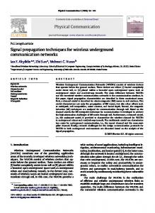
B. Discussion: Durations and Waiting Times Many authors include what they call service durations in their models. That means that they suppose that loading and unloading processes related to the various nodes of X require some time amount (x), (service time) and, so, that they distinguish, for any node x X, time values t(x) (beginning of the service) and t(x) + (x) (end of the service). By the same way, some authors suppose that the vehicles are always running at their maximal speed, and make a difference between the time t*(x), x X, when some vehicle arrives in x, and the time t(x) when this vehicle starts servicing the related demand (loading or unloading process). We do not do it. Taking into account service times, which tends to augment the size of the variables of the model and to make it more complex it, has really sense only if we suppose that the service times (x) depend on the current state (its current load) of the vehicle at the time the loading or unloading process has to be launched. Making explicitly appear waiting times t(x) – t*(x) is really useful if we make appear the speed profile as a component of the performance criterion. In case none of the situation holds, the knowledge of the routes of the vehicles and of the time value t(x), x X, is enough to check the validity of a given solution and to evaluate its performance, and then it turns out that ensuring the compatibility of the model with data which involve service times and waiting times t(x) – t*(x), x X, is only a matter of adapting the times windows F(x), the transit bounds (x), x X, and the distance matrix DIST (cf. Fig. 1).
Fig. 1 Considered times between two nodes
C. Modeling and Evaluation Techniques The model described in this section needs some definitions, we set: - First() = First element of ; Last() = last element of ; - for any z in : o Succ(, z) = Successor of z in ; o Pred(, z) = Predecessor of z in ; - for any z, z’ in : o z