Techniques for Efficient DCT/IDCT Implementation on Generic GPU Bo Fang*, Guobin Shen+, Shipeng Li+, and Huifang Chen* *
Dept. of Information Science & Electronic Eng., Zhejiang University, Hangzhou, P.R.China
[email protected],
[email protected]
Abstract—Emergence of programmable graphics processing unit has led to increasing interest in offloading numerically intensive computations on graphics hardware. DCT/IDCT is widely adopted in modern image/video compression standards and is usually one of the most computational expensive parts. In this paper, we present several techniques for efficient implementation of DCT/IDCT on generic programmable GPU, using direct matrix multiplication. Our experimental results demonstrate that the speed of IDCT on GPU with the proposed techniques can well exceed that on CPU with MMX optimization.
I.
INTRODUCTION
In recent years, high-performance Graphics Processing Unit (GPU) has become as ubiquitous as CPU. These GPUs have been equipped with significantly more computational power (e.g., much higher FLOPS) than CPU under same clock frequency. The performance of GPU continues to grow at an amazing rate, doubling every six months, which is much faster than the famous Moore’s Law for CPU [1]. Moreover, the programmability of graphics hardware is steadily increased, as a result, it allows efficient GPU implementations of general computations on commodity PCs [2~5]. We have developed efficient techniques to perform motion compensation (MC) on DirectX 8.0 compatible GPUs [6]. In this paper, we present several techniques that enable efficient implementation of DCT/IDCT on GPU. We believe this work is of more interesting since DCT/IDCT is more widely adopted than MC. For example, DCT/IDCT is widely adopted in most image compression standards such as JPEG and even the Motion JPEG video coding standards. Our work is based on Microsoft DirecX9.0 (DX9.0) and Shader Model 2.0 as they are supported by majority of modern graphics cards. All the shaders are programmed with Microsoft High-Level Shader Language (HLSL). Since the DCT is similar to the IDCT except the transform kernel is a transposed version, without loss of generality, we will only talk about IDCT in the following text while all the techniques can be applied to DCT directly. In fact, the proposed techniques can be applied to other block transforms as well. Furthermore, we use 8x8 IDCT as an example and it is straightforward to apply the proposed techniques to other sized IDCTs.
The work of this project iscompletely carried in Microsoft Research Asia during June to Sept. 2004.
+
Internet Media Group Microsoft Research Asia, Beijing, P.R.China
[email protected],
[email protected] The rest of the paper is organized as follows: in Section II, we briefly discuss the IDCT method to be used when implementing on GPU. Then several techniques for efficient IDCT on GPU are presented in Section III. The experimental results are shown in Section IV, followed by in-depth discussions. Finally, Section V concludes the paper and talks about the future work. II.
FAST ALGORITHMS VS DIRECT MATRIX MULTIPLICATION
There are many fast IDCT algorithms in the literature. However, all these fast algorithms are studied for efficient implementation of IDCT on Neumann processor such as CPU and the metric for efficiency is the number of multiplications and additions. Multiplication is significantly biased against additions since multiplication is considered much more expensive than addition. These fast algorithms have all implicitly assumed a cache-friendly implementation. No much memory I/O was considered: the input data is fetched only once for calculating all output data. On the other hand, GPU is a stream processor. A kernel program is independently run over a set of independent inputs. The internal graphics engine has four parallel channels and is indeed a SIMD processor. The multiplication, addition, multiplication and addition (mad) and even the dot product of two four-element vectors (dot) are of the same execution cost. All these features demand different fast IDCT algorithms for GPU implementation. While we are in searching for such fast algorithms, we apply direct matrix multiplication based implementation in this paper. One advantage of matrix multiplication is that the data access is highly regular. The 2D-IDCT is usually achieved using two 1D-IDCT using the row-column decomposition. In other words, the 2D-IDCT can be achieved via a left matrix multiplication and a right matrix multiplication (referred to as LeftX and RightX, respectively, hereafter for clarity), as shown in Eqn. (1) where C is the IDCT transform kernel.
X c = C ⋅ X ⋅ CT
(1)
Note that in most CPU based implementations, the row transform and the column transform are actually using the same routine since Eqn (1) can be re-written as Eqn (2) and
the transpose operation can be merged smartly into the transform routine.
X c = (C ⋅ (C ⋅ X )T )T
(2)
However, since the GPU does not have a memory addressing mode as flexible as that of CPU, we explicitly perform the LeftX and the RightX for the 2D-IDCT. III.
Routine 1 describes the pseudo PS code of the n-th rendering pass of the LeftX. TexCoord[8] are calculated by the VS and stores eight vertical adjacent source texels’ (a texel to a texture is a pixel to a picture) coordinates. LeftX_LMM{n}( TexCoord[8] ) //n = 0,1,…,7 { float color = 0 for i = 0 to 7 color += tex2D( srcTex, TexCoord[i] ) * IDCTCoef[n][i] end for
IDCT IMPLEMENTATION ON GPU
The computation on GPU is achieved through one or multiple rendering passes. The working flow of a rendering pass can be divided into two stages. In the first stage, a number of source textures, the associated vertex streams, the render target, the vertex shader (VS) and the pixel shader (PS) are specified. The source textures hold the input data. The vertex streams consist of vertices that contain the target position and the associated texture address information. The render target is a texture that holds the resulting IDCT results. The second stage is the rendering stage. The rendering is actually triggered after the DrawPrimitives call is issued. The vertex shader will calculate the target position and the texture address of each vertex involved in the specific primitive. Then the target texture is rasterized and the pixel shader is subsequently executed to perform per-pixel calculation. A. Different Rendering Mode of GPU There are quite a few rendering modes as determined by the primitive type (e.g., point, line, or triangle) used by the DrawPrimitives call. 1) Line mode multiplication For each pixel on the render target (i.e., a resulting pixel value after IDCT), it is obtained by performing the dot product of two corresponding vectors (one is the input DCT coefficient vector and the other is the IDCT transform kernel vector). Note that different target pixels correspond to different input vectors and IDCT transform kernel vectors. Since the IDCT transform kernel vectors are constant, they can be pre-calculated and stored into PS constants. However, the PS constants can not be altered during a render pass. Therefore, it is beneficial to render a span (i.e., a row or a column, depending on the LeftX or RightX) of target pixels at a time so that the IDCT transform kernel vectors can be shared and the requirement of re-loading the PS constants is avoided. To achieve this, we adopted the line rendering mode which renders a line at a time for the target texture. We call this technique Line Mode Multiplication (LMM). In the LeftX of LMM, there are eight rendering passes with each pass renders a row onto the target texture. The n-th pass renders the {8i + n}-th row for all the blocks (i = 0,1,…,H/8-1; H is the texture’s height). The vertex shaders for all the eight passes are the same while the pixel shaders are different in the constants only. The RightX is similar to the LeftX except that now each pass renders W/8 (W is the texture’s width) columns instead of H/8 rows. Clearly, the vertex streams for the RightX and the LeftX are different.
return color }
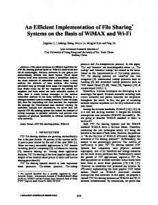
Routine 1. Pseudo PS code of LeftX of LMM. 2) Slice mode multiplication It is commonly recognized that the line rendering mode is not as efficient as triangle-based rendering mode due to the hardware design. To improve the efficiency, we developed a so-called Slice Mode Multiplication (SMM) scheme which enables one pass rendering based on triangle-based rendering mode. For this purpose, the IDCT transform kernel matrix must be stored in an 8x8 source texture for correct source texel and target pixel mapping. In the LeftX of SMM, eight rows can be rendered in one rendering pass. They compose a Wx8 (W-pixel wide and 8pixel high) slice. Each slice is identified by four vertices. The slice layout is shown in Fig. 1. The RightX of SMM is similarly performed except that slices are now 8xH rectangles.
Figure 1. Vertex definition in the LeftX of SMM. SMM differs from LMM in following aspects. Firstly, the matrix multiplication is accomplished in one rendering pass in SMM as compared with eight rendering passes in LMM. Secondly, much less vertices are involved ((W+H)/2 in SMM vs 2(W+H) in LMM) in each rendering pass. Thirdly, the IDCT transform kernel is stored in a texture in SMM, instead of storing in PS constants as in LMM. The first two differences significantly improve the efficiency of SMM because more pixels can be processed in parallel and the overhead of setups for rendering is reduced. However, the last difference actually brings in penalty in memory reads since the transform kernel needs to be read during the rendering process.
B. Multi-channel multiplication The internal graphics engine of GPU has four channels namely red, green blue, and alpha, that can work completely in parallel. Clearly, a good implementation should utilize this parallelism. Here we present a technique called Multichannel Multiplication (MCM) that utilizes the pixel level data parallelism. In MCM, the four neighboring pixels are “packed” into the four channels of a texel. Note that there is no need for the auxiliary packing and unpacking processes because the memory layout of a four-channel texel is exactly the same as that of four one-channel texels. Doing this way, the memory access instructions are significantly reduced since a single memory read will fetch four input data values. The LeftX of MCM is similar to that of LMM except that in MCM all the operations are in a four-channel fashion( i.e., SIMD). Thanks to the “packing”, a very powerful instruction, dot, which performs dot production of two four-element vectors, can be used in the RightX. This significantly saved the instruction count in the PS code which has a direct impact on the speed. Moreover, only two rendering passes are needed for the RightX. Routine 2 describes the pseudo PS code for the RightX of MCM. TexCoord[2] stores the two horizontal adjacent source texels’ coordinates. RightX_MCM{n}( TexCoord[2] ) //n = 0,1 { float4 src, color src = tex2D( srcTex, TexCoord[0] ) color.r = dot( src, IDCTCoef[n][0] color.g = dot( src, IDCTCoef[n][1] color.b = dot( src, IDCTCoef[n][2] color.a = dot( src, IDCTCoef[n][3] src = tex2D( srcTex, color.r += dot( src, color.g += dot( src, color.b += dot( src, color.a += dot( src,
) ) ) )
TexCoord[1] ) IDCTCoef[n][4] IDCTCoef[n][5] IDCTCoef[n][6] IDCTCoef[n][7]
the memory access becomes a severe bottleneck, as also observed in [7].
Figure 2. Repeated reading in LeftX of LMM To solve this problem, we utilize the capability of multiple render targets (MRT) of GPU. SM2.0 supports up to four rendering targets in a rendering pass. With MRT, if k (1