Nov 22, 2006 - of seabed characterisation (Chapman et al. ... Lloyd mirror effect (Jensen et al. .... simulated data generated for the GAIT workshop (Chapman.
Proceedings of ACOUSTICS 2006
20-22 November 2006, Christchurch, New Zealand
Techniques for extraction of the waveguide invariant from interference patterns in spectrograms Laura A. Brooks (1), M. R. F. Kidner (1)*, Anthony C. Zander (1), Colin H. Hansen (1) and Z. Yong Zhang (2) (1) School of Mechanical Engineering, The University of Adelaide, Australia (2) Maritime Operations Division, DSTO, Edinburgh SA 5111, Australia
ABSTRACT The determination of seabed properties from interference patterns (or striations) in frequency versus range spectrograms of shipping or other noise, depends on successful identification of these patterns. Within this paper, new local and global techniques for the extraction of the waveguide invariant from spectrogram striations are presented. The waveguide invariant relates the modal group and phase velocities of a medium and can be used as an input to an inversion model of the environment. The model can then be used to estimate seabed properties. The proposed methods apply to range-independent environments, such as continental shelves, and assume that the spectrogram data set is collected in the far field. By minimising the variance of the sound pressure level along the striations corresponding to assumed values of the waveguide invariant, the best fit with the actual waveguide invariant value is found. This paper compares the proposed striation determination methods and discusses the implementation aspects and robustness to noise of the new algorithms.
INTRODUCTION Seabed properties affect the propagation of sound in shallowwater environments and hence accurate modelling of the sea floor is necessary to predict sonar performance. Direct estimation is time-consuming, expensive and only accurate at the specific measurement location. Geoacoustic inversion techniques using acoustic measurements do not tend to suffer from these limitations and have become the preferred means of seabed characterisation (Chapman et al. 2003). Underwater activities requiring sonar often occur in shallow water regions in the vicinity of commonly used shipping and fishing routes, so noise generated by passing surface ships is frequent. The use of ship noise in geoacoustic inversions is therefore a potentially viable means of determining sea floor parameters. The benefits of using existing sound sources generated at remote locations are threefold: no additional sound, which has the potential to affect the behaviour of sea creatures (Richardson et al. 1995), is emitted into the underwater environment; no physical means of producing sonar sound, such as an air-gun, is needed; and the sensor, and ultimately any sea-vessel to which it is attached, becomes more difficult for a potentially hostile third party to detect. As a result of this, the development of inversion techniques using ship noise as a source has been of considerable interest in recent years (Heaney 2004b, Koch and Knobles 2005 and Park et al. 2005). D'Spain and Kuperman (1999) developed an analytical model, based upon the waveguide invariant, to predict the frequency dependence of broadband interference patterns in shallow water. Heaney (2004a, 2004b, 2004c) provides a method to extract three acoustic observables, one of them being the waveguide invariant, from a spectrogram and relates these to the sediment geoacoustic properties. Within this paper, the features observable on a spectrogram are highlighted. Subsequently, the problem of accurately Acoustics 2006
extracting information from the spectrogram, through the use of image and signal processing techniques, is discussed. Local and global techniques for the extraction of the waveguide invariant from a range independent environment spectrogram are presented, the computational efficiency and susceptibility of these techniques to background noise is explored, and the limitations of these techniques is discussed.
SPECTROGRAM FEATURES A spectrogram, such as the one depicted in Figure 1, is a visual representation of sound pressure as a function of frequency and range (or time). The most notable features of the plot are the striations (interference patterns), which are lines of constant (sound pressure) magnitude.
Figure 1. Example of a spectrogram generated from simulated data. The interference patterns are a function of the propagation characteristics of the environment and so can be used to determine the environmental properties. At close ranges, sound reflections from the sea surface may be 180 degrees out of phase with incident waves, cancelling out low frequency sounds. The difference in phase between the surface reflected path and the direct path changes significantly with range and hence the received sound level 1
20-22 November 2006, Christchurch, New Zealand
Proceedings of ACOUSTICS 2006
also varies significantly. This phenomenon, known as the Lloyd mirror effect (Jensen et al. 2000), is the main cause of the near-field striations; however, at ranges much further from the source, interaction between various modes and with the seafloor become more dominant. The range and frequency spacings of the striations are directly dependent upon the mutual interaction of the governing modes within the waveguide and the structure of the individual striations is dependent upon the group and phase velocities of the modes governing the sound propagation within the environment. Extracted striation features can therefore be used to estimate the governing modal model and subsequently related to the seafloor properties.
WAVEGUIDE INVARIANT The waveguide invariant (Brekhovskikh and Lysanov 1991), β, describes the dispersive characteristics of the field in a waveguide. It is defined as the ratio between the differential phase slowness, Sp, and the differential group slowness, Sg,
β =−
∂S p ∂S g
,
(1)
where the slowness is the reciprocal of the velocity. The waveguide invariants are generally positive for bottominteracting propagation and negative for refracting sound paths. For bottom-interacting propagation, the exact value of β will depend heavily upon the geoacoustic parameters of the sediment.
DATA SETS Three data sets were used to test and evaluate methods for extraction of the waveguide invariant: theoretical lines of constant magnitude; simulated waveguide data; and experimental waveguide data.
Theoretical lines of constant magnitude The first set of data, an example of which is depicted in Figure 2, consists of lines of constant magnitude, corresponding to a particular value of β and governed by Eq. (3). These represent striations. The example considered here has a waveguide invariant value of β =1.6, which is greater than would be expected in most realistic cases in which β tends to lie between –3 and 1 (Gerstoft et al. 2001). The higher value was chosen in this case to highlight the curvature of the lines which occurs at values of β not close to one (straight lines). The accuracy of the results obtained using this example are, however, applicable to all values of waveguide invariant. Lines of zero slope and constant magnitude and white Gaussian noise are used to represent tonals and background noise respectively. The main reason for testing any algorithm on this data set is because the simulated ‘striation’ lines are governed exactly by an analytical expression and hence any method used to calculate the waveguide invariant for this data set should be capable of calculating it exactly. The susceptibility of algorithms to the effects of adding tonals and various levels of background noise can also be easily analysed.
By considering the integration of the condition along a line of constant spectral level in a broadband spectrum, D'Spain and Kuperman (1999) derive the equation governing striation behaviour in a range independent environment (the seafloor and ocean properties are assumed to be constant as a function of the lateral distance from the source) to be:
β
r , r 0
ω = ω0
(2)
where r and ω are, respectively, the range and frequency at any point along the striation and (r0, ω0) refers to an arbitrary reference point, also located somewhere on the striation. Since β is constant for a range independent environment and ω0 and r0 are striation specific constants, Eq. (2) can be rewritten as:
ω = Cr β ,
(3)
where C is also a striation specific constant. The visual interpretation of this is a set of striation curves all emanating from an apparent origin of (r,f)=(0,0), where f=ω/2π. The curves will be convex if β > 1, concave if β < 1 and linear if β = 1. The normalised striation slope has been shown to approximate the waveguide invariant at sufficiently large ranges from the source in work presented previously by the authors (Brooks et al. 2006). This relationship can also be determined by differentiation of Eq. (3): lim
∆r →0 r
2
∆ω ∆r / =β . ω r
(4)
Figure 2. Simulated lines of constant magnitude with five tonals and -10 dB SNR (signal to noise ratio). Simulated data The spectrogram of data depicted graphically in Figure 1 is simulated data generated for the GAIT workshop (Chapman et al. 2003) as validation and verification test case 1. The simulation assumes a source located at a depth of 20 m in a range independent environment. The waveguide is 100 m deep and has a downward refracting sound speed profile with a constant c-2 gradient. The sediment is a single fluid layer. The simulated data is representative, yet contains no background noise or other disturbances. As a result, striations should be relatively easy to locate and characterise.
Experimental data The data set depicted in Figure 3 was collected in early April 2003 during sea trials carried out at a location approximately 8 nautical miles north of Rottnest Island, Western Australia. The trials were jointly conducted by DSTO (Defence Science and Technology Organisation) and the CMST (Centre for Acoustics 2006
Proceedings of ACOUSTICS 2006
20-22 November 2006, Christchurch, New Zealand
Marine Science and Technology). The data set was recorded on a single hydrophone located within the 34 m deep waveguide at a depth of 24 metres during a run of the deployment vessel Total Warrior. The environment is assumed to be range independent. Since data sets from only one hydrophone were used, array processing of the data could not be undertaken. The signal to noise ratio (SNR) is therefore low. As a result, the experimental data provide a good means to test the algorithm because the striations are more difficult to identify than would generally be the case for experimental array data.
Figure 4. Geometry for determination of waveguide invariant at point (r,ω). Alternative local technique
Figure 3. Experimental data recorded from a passing ship during the 2003 Rottnest Island trials.
EXTRACTION OF THE WAVEGUIDE INVARIANT Many of the available experimental data sets contain tonal noise of high amplitude relative to the peaks of the striations. These tones can be removed from the spectra by extraction of a smoothed data set from the original. Smoothing the data in the range axis is achieved through convolution of the amplitude matrice with a vector of ones and subtraction of the result from the original data. Within this section, four methods for the extraction of the waveguide invariant in a range independent environment are described: two local techniques and two global techniques.
Basic local technique The quickest and simplest method for determining the waveguide invariant is through determination of the normalised striation slope at ranges sufficiently far from the source location. The spectrogram data set is low-pass filtered to minimise the effects of background and tonal noise. The normalised striation slope at any point is then approximated as the ratio of the normalised frequency spacing between adjacent striations and the normalised range spacing between adjacent striations at that point, as defined mathematically in Eq. (4), and depicted graphically in Figure 4. An advantage of this technique is that it can be used in both range dependent and range independent environments. The main disadvantage of this technique is that tonals and high levels of background noise can make location of the individual striations difficult. If a striation is missed or if a false striation is picked up the results will be highly erroneous. Errors will also occur if the (r, ω) point at which the calculation is made is not located centrally in both range and frequency between the two adjacent striations. In addition, inaccuracies may also occur in the vicinity of cut-on frequencies due to the formation of new striations above these frequencies.
Acoustics 2006
A second method for the identification of the local slope of the striations uses the autocorrelation of small areas from the spectrum. The peaks in the autocorrelation lie along lines of the same angle as the striation. Once the peak data are extracted, a least squares fit to the data can be made and the equation of the line identified. If this process is repeated over the entire spectrogram an estimate of the local gradient, as a function of range and frequency, can be formed. The method consists of the following steps. 1.
Tonals and the geometric spreading from the data are removed as described in the first paragraph of the ‘extraction of the waveguide invariant’ section.
2.
The data set is plotted on logarithmic axes, so that the striations become straight lines with equations of the form
ln ( f ) = β ln (r ) + C1 ,
(5)
where C1 is a striation specific constant. 3.
The image is divided into square segments of M x M pixels. For each of these segments the M-point autocorrelation is evaluated. This yields new segments of size 2M-1 x 2M-1 pixels.
4.
Peak data from the autocorrelations of each segment are extracted.
5.
A straight line is fitted to the data in a least squares sense, using the cross- and auto-covariances of the frequency and range coordinates of the peak points (all points greater than a pre-determined threshold).
6.
The best-fit line gradients are averaged and a mean value for the waveguide invariant is obtained.
3
20-22 November 2006, Christchurch, New Zealand
Proceedings of ACOUSTICS 2006
Exhaustive global technique Greater accuracy can be obtained using a global algorithm. Suitable frequency and range extents over which the algorithm is to be applied are selected and the value of C at N evenly spaced points along the main diagonal connecting (rmin, fmax) to (rmax, fmin) is evaluated at I different values of β:
ω
Ci , n = βn0 , rn 0i
where i = 1:I,
(6)
and where
rn0 = rmin +
n(rmax − rmin ) , N −1
(7)
and
ω n0 = 2πf n0 = 2π f max −
n( f max − f min ) , N −1
(8)
define the range and frequency locations, respectively, of the nth point on the diagonal. For each value of C, K points, defined by (rin(k), ωin(k)), along lines governed by this value:
ω in( k ) = C i ,n rin( k )
β i , where n = 1:N and k = 1:K,
(9)
are selected and the amplitude at each of these points, A(rin(k), ωin(k)), is determined. The amplitude variance, σn,i2, along each of the n lines governed by C is determined and the mean variance of the amplitude, µi,σ , is calculated for each value of i. The minimum mean variance most likely corresponds to the true value of the waveguide invariant. The reason for this is that lines governed by the true value of β are relatively constant in amplitude and therefore exhibit a low variance, whilst lines that don’t correspond to the true value of β experience significant changes in amplitude as they cut across the striation minima and maxima. A graphical representation of the geometry for this algorithm is depicted in Figure 5.
hydrophone and cylindrical spreading is assumed at ranges greater than this. The resulting geometric spreading model is:
TLGS = 10 log(r ) + 20 log(z r ) − 10 log(z r ) ,
(10)
where TLGS is the transmission loss due to geometric spreading, and zr is the depth of the receiving hydrophone. By applying Eq. (10), the geometrical spreading effect is approximately removed from the spectrogram data before the exhaustive global algorithm is applied. Determination of the equation governing striation behaviour enables the striations to be linearised for subsequent processing. Once the waveguide invariant is known, if further analysis is desired, the linearised range can be set to equal rβ. Individual striations can then be more easily identified using classical line detection techniques. Although this technique can exhibit a high degree of accuracy when sufficient points are sampled, its exhaustive nature results in a computationally intensive problem.
Global technique with optimisation In order to improve the computational efficiency of the global technique algorithm, pre-processing and optimisation techniques are employed. Both the original cost function described in the previous section (minimisation of the mean variance of the amplitude along striation lines), and an alternative cost function (minimisation of the mean value along the striation minima), are tested. During pre-processing, geometric spreading is accounted for by application of Eq. (10). The magnitude of the spectra is then converted from dB into linear values to emphasise the dynamic range. It is then low pass filtered in both the range and frequency directions (by convolving the spectrogram amplitude matrix with an Nf × Nr matrix of ones, where Nf and Nr define the amount of low pass filtering in the frequency and range directions respectively). A threshold value is selected and values above this value are set to the maximum value. This is done as these values will otherwise dominate the result. Filtering (through convolution) is then applied once again to eliminate any small regions of very low level. Figure 6 displays an example of the pre-processing as applied to the experimental data. It can be seen that the preprocessing highlights the data near the striations.
Figure 5. Geometry for waveguide invariant determination using exhaustive global technique. Any realistic acoustic data will exhibit transmission loss, mainly due to a combination of geometric spreading and attenuation. The amplitude along a striation will therefore decrease with range, resulting in a greater variance along the striation. This variance can be decreased by minimisation of the geometric spreading effects. Spherical spreading is assumed at ranges less than the depth of the receiving
4
Figure 6. Pre-processed experimental data. A Matlab nonlinear function minimisation based on golden section search and parabolic interpolation (the Matlab algorithm is virtually the same as the Fortran version presented by Forsythe et al. 1976) is employed in order to minimise the cost function within the waveguide invariant range over which the search is applied. If the original cost function is used, the mean variance of the TL along lines Acoustics 2006
Proceedings of ACOUSTICS 2006
20-22 November 2006, Christchurch, New Zealand
passing through a set of n points spaced evenly in the range dimension is determined. If the alternative cost function is used, values that are less than a certain threshold value are chosen as values likely to lie on or near a striation minimum. The value of C at each of these points is evaluated and the average of the mean value of the TL along each line governed by the calculated C values is determined.
frequencies of 100 Hz to 400 Hz. Application of the technique to this data set produced waveguide invariant approximations of between about 2.0 and 3.6, which is well above the expected value of 1.6. The main reason for this was the difficulty in determining the striation maxima. Many maxima were inadvertently omitted and some erroneous maxima were classed as maxima.
The optimisation techniques employed are more accurate when applied to functions that are sufficiently smooth. Therefore, application to real data that had not been preprocessed (i.e. not smoothed) would have a greater likelihood of producing erroneous results.
Attempts at applying the method to the experimental data were undertaken, however no reasonable results could be obtained using this method.
APPLICATION OF ALGORITHMS The algorithms described within this paper: basic local technique; alternative local technique; exhaustive global technique; and global technique with optimisation, were applied to the three data sets (representative theoretical, simulated and experimental). Aspects of the algorithms which were considered include: accuracy of the results obtained; computational efficiency; robustness to noise; and sensitivity to user-defined input parameters.
Although the results obtained were poor, it is likely that the accuracy could be increased if more complex signal processing techniques were incorporated into the algorithm.
Alternative local technique The alternative local technique was applied to the Rottnest Island experimental data set. The data in the range dimension were smoothed to correct for tonals (step 1 of the described technique). The original, smoothed and difference data for this case are depicted in Figure 7. Figures 8-10 depict the data after application of steps 2, 3 and 5, respectively, of the described technique.
Basic local technique Each of the three data sets was low pass filtered. The normalised striation slope was determined at a number of evenly spaced locations and the waveguide invariant was then approximated as the mean value. The calculation points chosen for the theoretical lines of constant magnitude lay on the grid defined by ranges from 1000 m to 4000 m and by frequencies of 100 Hz to 400 Hz. The mean waveguide invariant value obtained was highly dependent upon the number of locations used in the measurement. A sample of the results obtained for various range and frequency increment values is depicted in Table 1.
Table 1. Mean waveguide invariant value obtained for theoretical lines of constant magnitude. Mean value of Range Frequency Total no. waveguide increment increment measurements invariant 950 104 9 1.216 1000 100 12 1.231 500 100 20 1.096 1000 50 21 2.230 1000 25 39 1.892 500 40 40 1.485 400 25 78 1.942 200 40 88 1.922 100 40 168 1.509 100 20 336 1.543 50 10 1271 1.763 20 25 1313 2.016 20 4 7676 2.044 The values are, in many cases, dissimilar to the actual waveguide invariant value of 1.6. There are several possible reasons for these discrepancies: the existence of tonals, which may sometimes be mistaken for striations; the fact that the location at which an average is taken is rarely centred evenly between two striations; the existence of background noise; and the fact that the assumption of the waveguide invariant being equal to the normalised striation slope is only an approximation. The calculation points chosen for the simulated data lay on the grid defined by ranges from 2000 m to 3000 m and by Acoustics 2006
(a)
(b)
(c)
Figure 7. Noise removal by subtraction of smoothed data. The images are: a) the original spectrogram, b) the smooth spectrogram, and c) the difference of the two.
Figure 8. Pixel maps of the experimental spectrogram data plotted against log freq and log range showing a) raw data, b) smoothed data, c) difference of the two. The squares in image (c) indicate the locations at which the autocorrelation was evaluated. The results are depicted in Figure 9. 5
20-22 November 2006, Christchurch, New Zealand
Figure 9. The autocorrelation over 128 data points at three locations on the clean spectrogram data. The locations, which are highlighted in Figure 8, are a) at the top of the image, b) in the region with definite downward stripes, and c) in the region with upward and rightward stripes.
Proceedings of ACOUSTICS 2006
that the waveguide invariant value is successfully determined to be the true value of 1.6 for a SNR of -10 dB. Decreasing the SNR results in a less smooth curve (see Figures 11b-11c), however the correct value of waveguide invariant is still determined when the SNR is -30 dB. At even lower SNRs however, the noise levels become too high and the waveguide invariant can no longer be successfully determined (see Figure 11d). Although there is a dip in the variance around the true value of β, the local minimum here is not an obvious solution for the waveguide invariant. This can be explained by considering the amplitude difference that results from constructive interference along lines other than that determined by the true value of the waveguide invariant. When the SNR is high, this amplitude difference is also high, whilst the amplitude along the striations is relatively constant, resulting in a noticeable increase in variance for test waveguide invariant values that define lines further from the true striation line. Once the SNR becomes too low, noise dominates the constructive interference effects and hence it is impossible to tell whether the line of interest passes through areas of changing amplitude that are due to modal interference, or whether this amplitude variance is due to noise.
(a)
(b)
Figure 11a. Variance along striations as a function of waveguide invariant for theoretical data with a SNR of –10 dB.
(c)
Figure10. Best fit lines to the local autocorrelation functions. The resulting slopes for each of the correlation functions are
β = 0.9534, β = -0.8192 and β = 0.0114. The first value, from
the autocorrelation of the data in the clearest region is fairly close to the approximately unity value of β expected.
Exhaustive global technique
Figure 11b. Variance along striations as a function of waveguide invariant for theoretical data with a SNR of -20 dB.
The exhaustive global technique was applied to each of the three data sets. Theoretical constant magnitude lines representing a range of waveguide invariants with various tonals and levels of background noise were successfully tested. The algorithm was shown to be highly robust to background noise. As an example, Figure 11 shows the results obtained when eight lines of constant magnitude representing a waveguide invariant of 1.6 with tonals at 70, 150, 220, 290 and 460 Hz were used. Figure 11a indicates 6
Acoustics 2006
Proceedings of ACOUSTICS 2006
Figure 11c. Variance along striations as a function of waveguide invariant for theoretical data with a SNR of -30 dB.
Figure 11d. Variance along striations as a function of waveguide invariant for theoretical data with a SNR of -40 dB. The exhaustive global algorithm was also successfully applied to both the simulated and experimental data. Waveguide invariant values of 0.95 and 1.1, respectively, were determined, as can be seen from Figures 12 and 13. The accuracy of the technique appears to be high as the β = 0.95 value determined for the simulated data is the same as that which was used to simulate the data and the β = 1.1 value obtained for the experimental data lies within the region of that approximated for the real data set. The variance curve in Figure 13 can be smoothed by low-pass filtering the data in both the range and frequency dimensions; however, the same waveguide invariant value is determined using the exhaustive global search algorithm regardless of whether or not this smoothing operation is performed.
20-22 November 2006, Christchurch, New Zealand
Figure 13. Variance along striations as a function of waveguide invariant for experimental data. Although the exhaustive global algorithm has been successfully applied to all three range independent data sets, it does have the inherent drawback of being computationally intensive. Running the algorithm on a 3 GHz Pentium 4 with 512 MB RAM takes 145 seconds when applied to the theoretical lines of constant magnitude data, 405 seconds for the simulated data and 159 seconds for the experimental data. The computational time can be decreased by reducing the number of points over which the search takes place; however, this has the potential to negatively affect the accuracy of the results. A second drawback of the exhaustive global technique is that the waveguide invariant is only determined at increments of 0.05. Decreasing this increment in order to improve the accuracy of the determined value also increases the computational time significantly.
Global technique with optimisation Application of the global technique to simulated data using the original cost function (minimisation of the mean variance of the amplitude along striation lines) resulted in a waveguide invariant of 0.9266, which is slightly less than, but similar to, the value determined using the exhaustive technique. The computational time of 16 seconds is far quicker than that of the exhaustive technique. However, application of the global technique using the alternative cost function (minimisation of the mean value along the striation minima) proved to be more difficult. The results obtained were found to be strongly dependent upon the extent to which each dimension was filtered, the threshold value above which all values were set to a maximum, the function minimisation routine selected, and the number of minima over which the search was conducted. Reasonable input values resulted in waveguide invariant values ranging between 0.88 and 1.11. Application of both the original and alternative cost functions to the experimental data produced results which were highly dependent upon the aforementioned input parameters. Although the true waveguide invariant value was determined for some parameters, other valid parameter choices resulted in highly erroneous results.
CONCLUSION
Figure 12. Variance along striations as a function of waveguide invariant for simulated data.
Acoustics 2006
The proposed global method for determining the waveguide invariant from range independent data has the advantages over the proposed local techniques in that it is able to produce accurate results, and overcome tonal interference, high levels of background noise, and large variations in striation width, without the necessity of significant additional processing of the data.
7
20-22 November 2006, Christchurch, New Zealand
Minimisation of the variance along the striations has been shown to be an effective means of obtaining results from simulated data.
Proceedings of ACOUSTICS 2006
Richardson, W. J., Greens, C. R., Malme, C. I. and Thomson, D.H. 1995, Marine Mammals and Noise, Academic, San Diego.
The use of optimisation techniques after pre-processing the data has been shown to be more computationally efficient than exhaustive techniques, but inaccuracies were observed in the results obtained. Further research into the optimal choice of cost function and optimisation algorithm is currently being undertaken. The goal of the current investigations is to produce a robust algorithm that is computationally efficient, yet still able to produce results equivalent in accuracy to those produced by the exhaustive global method.
ACKNOWLEDGEMENT The authors would like to thank the DSTO (Defence Science and Technology Organisation) for their contributions and also Paul Clarke for useful discussions.
REFERENCES Brekhovskikh, L. and Lysanov, Y. 1991, Fundamentals of Ocean Acoustics, 2nd edn. Springer-Verlag, Berlin. Brooks, L.A., Kidner, M.R.F., Zander, A.C., Hansen, C.H. and Zhang, Z.Y. 2006, ‘Striation processing of spectrogram data’, Proceedings of the Thirteenth International Congress on Sound and Vibration, July 2-6 Vienna, Austria. Chapman, R., Chin-Bing, S., King, D. and Evans, R.B. 2003, ‘Benchmarking geoacoustic inversion methods for rangedependent waveguides’, IEEE Journal of Oceanic Engineering, vol. 28, no. 3, pp 320-330. D’Spain, G.L. and Kuperman, W.A. 1999, ‘Application of waveguide invariants to analysis of spectrograms from shallow water environments that vary in range and azimuth’, Journal of the Acoustical Society of America, vol. 106, no. 5, pp 2454-2468. Forsythe, G.E., Malcolm, M.A. and Moler, C.B. 1976, Computer Methods for Mathematical Computations, Prentice-Hall. Gerstoft, P., D’Spain, G.L., Kuperman, W.A. and Hodgkiss, W.S. 2001, ‘Calculating the waveguide invariant beta by ray-theoretic approaches’, MPL Tech. Memo. TM-468, Marine Physical Laboratory, University of California, San Diego. Heaney, K.D. 2004, ‘Rapid geoacoustic characterization: Applied to range-dependent environments’, IEEE Journal of Oceanic Engineering, vol. 29, no. 1, pp 43-50. Heaney, K.D. 2004, ‘Rapid geoacoustic characterization using a surface ship of opportunity’, IEEE Journal of Oceanic Engineering, vol. 29, no. 1, pp 88-99. Heaney, K.D., Sternlicht, D.D., Teranishi, A.M., Castile, B. and Hamilton, M. 2004, ‘Active rapid geoacoustic characterization using a seismic survey source’, IEEE Journal of Oceanic Engineering, vol. 29, no. 1, pp 100109. Jensen, F.B., Kuperman, W.A., Porter, M.B. and Schmidt, H. 2000, Computational Ocean Acoustics, Springer-Verlag New York Inc., USA. Koch, R. and Knobles, D. 2005, ‘Geoacoustic inversion with ships as sources’, Journal of the Acoustical Society of America, vol. 117, no. 2, pp 626-637. Park, C., Seong, W. and Gerstoft, P. 2005, ‘Geoacoustic inversion in time domain using ship of opportunity noise recorded on a horizontal towed array’, Journal of the Acoustical Society of America, vol. 117, no. 4, pp 19331941.
8
Acoustics 2006