Template Semantics

Template Semantics: A Parameterized Approach to Semantics-Based Model Compilation by

Jianwei Niu

A thesis presented to the University of Waterloo in fulfilment of the thesis requirement for the degree of Doctor of Philosophy in Computer Science

Waterloo, Ontario, Canada, 2005

c Jianwei Niu 2005

I hereby declare that I am the sole author of this thesis. I authorize the University of Waterloo to lend this thesis to other institutions or individuals for the purpose of scholarly research.

Jianwei Niu

I further authorize the University of Waterloo to reproduce this thesis by photocopying or other means, in total or in part, at the request of other institutions or individuals for the purpose of scholarly research.

Jianwei Niu ii

Abstract This dissertation discusses a parameterized approach to the compiling of model-based notations into input languages of formal-analysis tools, based on descriptions of the notations’ semantics. The semantics of a model-based notation is complex, and formalizing it in a semantics-description language, such as structural operational semantics and higher-order logic, can be challenging and error-prone. We propose a new approach, called template semantics, to structure the semantics of model-based specification notations. We demonstrate how to use template-semantics descriptions to construct notation-specific model compilers, which ease the mapping of new notations or notation variants to analysis tools. The basic computation model of template semantics is a non-concurrent, hierarchical transition system (HTS), whose execution semantics are parameterized. Semantics that are common among notations, e.g., the concept of an enabled transition are captured in the template, and a notation’s distinct semantics, e.g., which events can enable transitions, are specified as parameters. HTSs can be combined by composition operators to form more complex, concurrent specifications. We provide the template semantics of seven composition operators and some of their variants; the operators define how multiple HTSs execute concurrently and how they communicate and synchronize with each other by exchanging events and data. The definitions of these operators use the template parameters to preserve notation-specific behaviour in composition. By separating a notation’s step semantics from its composition operators, we simplify the definitions of both.

iii

Template semantics is employed to capture succinctly the semantics of basic transition systems, CSP, CCS, basic LOTOS, a variety of statecharts notations, a subset of SDL88, SCR, and Petri Nets. We demonstrate also that template semantics can handle some sophisticated notation features, such as statecharts’ history states and SDL’s timing conditions. The template-semantics description for a notation is an instantiation of the template parameters, which focus on differences and similarities among notations. Therefore, template semantics eases a user’s effort in understanding a notation and in comparing notation variants. We introduce a parameterized model compiler, which takes as input the description of a notation’s template semantics and transforms a specification in that notation into a transition relation, which can be checked by formal-analysis tools, such as model checkers.

iv

Acknowledgements I would like to express my deep gratitude to my supervisors, Professor Joanne M. Atlee and Professor Nancy A. Day, for their guidance, knowledge, patience, time, and energy, which have been invaluable to my Ph.D. research and the writing of my thesis. Special thanks to my committee members, Professor Daniel Berry, Professor Betty H. C. Cheng, Professor Andrew J. Malton, and Professor John G. Thistle, for taking their precious time to review this thesis and provide valuable comments. In addition, I appreciate the academic and spiritual support of the members of the WatForm research group. My friends, Professor Ming Li, Luosha Lu, Professor Bin Ma, Weiming Zhang, Fang Wei, Haihong Zhang, Mei Zhou, Jiongxiong Chen, Yinghua Jia, Yun Lu, Yuan Peng, and Ann Zimmer, have made my years at Waterloo truly enjoyable. Most of all, I thank my mother and my sister who have consistently given me their unconditional love. None of this would have been possible without my husband, Zhiwei, who has sat up at night with me and cared for our newborn son, Jeffrey, who has brought us so much joyfulness. I cannot find the words to express my gratefulness for Zhiwei’s love, understanding, and support. I am also very grateful for the financial support of the Natural Sciences and Engineering Research Council (NSERC), the Ontario Graduate Scholarship in Science and Technology (OGSST), and the University of Waterloo.

v

I dedicate my thesis to the memory of my father who was always proud of me and believed that I was capable of achieving all of my goals. He was not only the best father, but also my best teacher and my best friend.

vi

Contents

1 Introduction 1.1

1

Automated Analysis Methods . . . . . . . . . . . . . . . . . . . . . . . . .

3

1.1.1

Notation-Specific Analysis Tools . . . . . . . . . . . . . . . . . . . .

3

1.1.2

Translation to an Existing Analyzer . . . . . . . . . . . . . . . . . .

3

1.1.3

Semantics-Based Approaches . . . . . . . . . . . . . . . . . . . . . .

5

1.1.4

Terminology . . . . . . . . . . . . . . . . . . . . . . . . . . . . . . .

6

Thesis Overview . . . . . . . . . . . . . . . . . . . . . . . . . . . . . . . . .

8

1.2.1

Template Semantics

. . . . . . . . . . . . . . . . . . . . . . . . . .

9

1.2.2

Parameterized Model Compiler . . . . . . . . . . . . . . . . . . . .

11

1.3

Contributions . . . . . . . . . . . . . . . . . . . . . . . . . . . . . . . . . .

16

1.4

Thesis Validation . . . . . . . . . . . . . . . . . . . . . . . . . . . . . . . .

17

1.5

Overview of Dissertation . . . . . . . . . . . . . . . . . . . . . . . . . . . .

19

1.2

2 Related Work

21

2.1

Semantics of Model-Based Notations . . . . . . . . . . . . . . . . . . . . .

21

2.2

Automated Analysis of Model-Based Notations

23

vii

. . . . . . . . . . . . . . .

2.3

2.4

2.5

Translation from Notations to Analysis Tools . . . . . . . . . . . . . . . . .

24

2.3.1

Translation Between Two Notations . . . . . . . . . . . . . . . . . .

24

2.3.2

Intermediate Languages . . . . . . . . . . . . . . . . . . . . . . . .

25

Semantics-Based Approaches . . . . . . . . . . . . . . . . . . . . . . . . . .

27

2.4.1

Fusion . . . . . . . . . . . . . . . . . . . . . . . . . . . . . . . . . .

27

2.4.2

Hypergraph . . . . . . . . . . . . . . . . . . . . . . . . . . . . . . .

28

2.4.3

Amalia . . . . . . . . . . . . . . . . . . . . . . . . . . . . . . . . . .

29

Summary . . . . . . . . . . . . . . . . . . . . . . . . . . . . . . . . . . . .

30

3 Hierarchical Transition Systems (HTSs)

31

3.1

Syntax of HTSs . . . . . . . . . . . . . . . . . . . . . . . . . . . . . . . . .

31

3.2

Semantics of HTSs . . . . . . . . . . . . . . . . . . . . . . . . . . . . . . .

36

3.2.1

Snapshots . . . . . . . . . . . . . . . . . . . . . . . . . . . . . . . .

37

3.2.2

Micro-Step Semantics . . . . . . . . . . . . . . . . . . . . . . . . . .

38

3.2.3

Macro-Step Semantics . . . . . . . . . . . . . . . . . . . . . . . . .

41

3.2.4

Initial Snapshots . . . . . . . . . . . . . . . . . . . . . . . . . . . .

46

Template Parameters . . . . . . . . . . . . . . . . . . . . . . . . . . . . . .

46

3.3.1

States . . . . . . . . . . . . . . . . . . . . . . . . . . . . . . . . . .

49

3.3.2

Events . . . . . . . . . . . . . . . . . . . . . . . . . . . . . . . . . .

51

3.3.3

Variable Values . . . . . . . . . . . . . . . . . . . . . . . . . . . . .

55

3.3.4

Priority . . . . . . . . . . . . . . . . . . . . . . . . . . . . . . . . .

59

Summary . . . . . . . . . . . . . . . . . . . . . . . . . . . . . . . . . . . .

60

3.3

3.4

viii

4 Composition Operators 4.1

4.2

4.3

4.4

4.5

61

General Aspects of Composing Components . . . . . . . . . . . . . . . . .

61

4.1.1

Composition Hierarchy . . . . . . . . . . . . . . . . . . . . . . . . .

62

4.1.2

Snapshot Hierarchy . . . . . . . . . . . . . . . . . . . . . . . . . . .

64

4.1.3

Initial Snapshots . . . . . . . . . . . . . . . . . . . . . . . . . . . .

66

Micro-Step Composition Semantics . . . . . . . . . . . . . . . . . . . . . .

66

4.2.1

Substitution . . . . . . . . . . . . . . . . . . . . . . . . . . . . . . .

67

4.2.2

Step Abbreviations . . . . . . . . . . . . . . . . . . . . . . . . . . .

68

4.2.3

Update, Communicate, and Communicate vars Predicates . . . . .

70

Macro-Step Composition Semantics . . . . . . . . . . . . . . . . . . . . . .

74

4.3.1

Inferred Macro-Step Composition . . . . . . . . . . . . . . . . . . .

74

4.3.2

Stable Snapshot Trees . . . . . . . . . . . . . . . . . . . . . . . . .

75

Composition Operators . . . . . . . . . . . . . . . . . . . . . . . . . . . . .

76

4.4.1

Parallel . . . . . . . . . . . . . . . . . . . . . . . . . . . . . . . . .

76

4.4.2

Interleaving . . . . . . . . . . . . . . . . . . . . . . . . . . . . . . .

80

4.4.3

Environmental Synchronization . . . . . . . . . . . . . . . . . . . .

81

4.4.4

Rendezvous Synchronization . . . . . . . . . . . . . . . . . . . . . .

85

4.4.5

Sequence . . . . . . . . . . . . . . . . . . . . . . . . . . . . . . . . .

89

4.4.6

Choice . . . . . . . . . . . . . . . . . . . . . . . . . . . . . . . . . .

90

4.4.7

Interrupt . . . . . . . . . . . . . . . . . . . . . . . . . . . . . . . . .

91

Summary . . . . . . . . . . . . . . . . . . . . . . . . . . . . . . . . . . . .

94

5 Parameterized Model Compiler

95

ix

5.1

Concept of Model Compilers . . . . . . . . . . . . . . . . . . . . . . . . . .

96

5.2

Parameterized Semantics-Based Model Compiler . . . . . . . . . . . . . . .

96

5.2.1

Structure of Metro . . . . . . . . . . . . . . . . . . . . . . . . . . .

98

5.2.2

Characteristic Predicate Representation of Sets . . . . . . . . . . . 101

5.2.3

Existential Quantification . . . . . . . . . . . . . . . . . . . . . . . 102

5.3

5.4

Implementation . . . . . . . . . . . . . . . . . . . . . . . . . . . . . . . . . 103 5.3.1

Representation of Syntax . . . . . . . . . . . . . . . . . . . . . . . . 103

5.3.2

Representation of Snapshots . . . . . . . . . . . . . . . . . . . . . . 106

5.3.3

Representation of Step Semantics . . . . . . . . . . . . . . . . . . . 108

5.3.4

Semantic Functions for HTS Syntax . . . . . . . . . . . . . . . . . . 112

5.3.5

Representation of Composition Operators . . . . . . . . . . . . . . 114

5.3.6

Scope of Implementation . . . . . . . . . . . . . . . . . . . . . . . . 122

5.3.7

Testing and Inspection of Implementation . . . . . . . . . . . . . . 123

5.3.8

Limitations . . . . . . . . . . . . . . . . . . . . . . . . . . . . . . . 123

Summary . . . . . . . . . . . . . . . . . . . . . . . . . . . . . . . . . . . . 124

6 Validation 6.1

6.2

125

Case Studies . . . . . . . . . . . . . . . . . . . . . . . . . . . . . . . . . . . 126 6.1.1

Heating System . . . . . . . . . . . . . . . . . . . . . . . . . . . . . 127

6.1.2

Single-Lane-Bridge System . . . . . . . . . . . . . . . . . . . . . . . 133

Model Checking Results . . . . . . . . . . . . . . . . . . . . . . . . . . . . 138 6.2.1

State Spaces of Case Studies . . . . . . . . . . . . . . . . . . . . . . 140

6.2.2

Case Studies Using Metro . . . . . . . . . . . . . . . . . . . . . . . 142

x

6.2.3

Case Studies Using Express . . . . . . . . . . . . . . . . . . . . . . 143

6.3

Methodology . . . . . . . . . . . . . . . . . . . . . . . . . . . . . . . . . . 144

6.4

Additional Notations and Advanced Features . . . . . . . . . . . . . . . . . 147 6.4.1

SCR . . . . . . . . . . . . . . . . . . . . . . . . . . . . . . . . . . . 147

6.4.2

SDL . . . . . . . . . . . . . . . . . . . . . . . . . . . . . . . . . . . 158

6.4.3

Petri Nets . . . . . . . . . . . . . . . . . . . . . . . . . . . . . . . . 166

6.4.4

Advanced features . . . . . . . . . . . . . . . . . . . . . . . . . . . 170

6.5

Comparison of Notations . . . . . . . . . . . . . . . . . . . . . . . . . . . . 180

6.6

Summary . . . . . . . . . . . . . . . . . . . . . . . . . . . . . . . . . . . . 188

7 Concluding Remarks and Future Work

189

7.1

Contributions . . . . . . . . . . . . . . . . . . . . . . . . . . . . . . . . . . 190

7.2

Limitations . . . . . . . . . . . . . . . . . . . . . . . . . . . . . . . . . . . 193

7.3

Future Work . . . . . . . . . . . . . . . . . . . . . . . . . . . . . . . . . . . 194

Bibliography

197

A Specification of Single-Lane-Bridge System

207

B Specification of Heating System

227

xi

List of Tables 3.1

HTS accessor functions . . . . . . . . . . . . . . . . . . . . . . . . . . . . .

35

3.2

Parameters to be provided by template user . . . . . . . . . . . . . . . . .

48

3.3

Sample definitions for state-related template parameters . . . . . . . . . .

50

3.4

Sample definitions for event-related template parameters . . . . . . . . . .

52

3.5

Sample definitions for variable-related template parameters . . . . . . . . .

57

3.6

Sample definitions for priority template parameter . . . . . . . . . . . . . .

60

4.1

Predicates for event communication . . . . . . . . . . . . . . . . . . . . . .

71

6.1

Template parameters and compositions operators for statecharts variants (“n/a” means “not applicable”) . . . . . . . . . . . . . . . . . . . . . . . . 132

6.2

Template parameters and compositions operators for process algebras and BTSs notations (“n/a” means “not applicable”) . . . . . . . . . . . . . . . 139

6.3

Statistics for heating system . . . . . . . . . . . . . . . . . . . . . . . . . . 140

6.4

Statistics for single-lane-bridge system . . . . . . . . . . . . . . . . . . . . 141

6.5

Template parameters for statecharts variants (“n/a” means not applicable)

6.6

Possible macro-steps of Harel’s and Maggiolo-Schettini’s Statecharts

xii

182

. . . 187

6.7

Possible macro-steps of STATEMATE . . . . . . . . . . . . . . . . . . . . 187

6.8

Possible macro-steps of RSML . . . . . . . . . . . . . . . . . . . . . . . . . 187

6.9

Possible macro-steps of UML state model . . . . . . . . . . . . . . . . . . . 187

xiii

List of Figures 1.1

Notation-specific model checker . . . . . . . . . . . . . . . . . . . . . . . .

4

1.2

Translation from a specification notation to a model checker . . . . . . . .

5

1.3

Semantics-based approach . . . . . . . . . . . . . . . . . . . . . . . . . . .

6

1.4

Parameterized model compiler

. . . . . . . . . . . . . . . . . . . . . . . .

13

1.5

Express: Parameterized translator . . . . . . . . . . . . . . . . . . . . . . .

15

3.1

Example showing state hierarchy in an HTS . . . . . . . . . . . . . . . . .

34

3.2

A stable macro-step of an HTS . . . . . . . . . . . . . . . . . . . . . . . .

45

4.1

An example composition tree . . . . . . . . . . . . . . . . . . . . . . . . .

63

4.2

An example CHTS . . . . . . . . . . . . . . . . . . . . . . . . . . . . . . .

63

4.3

A snapshot tree for component com3 . . . . . . . . . . . . . . . . . . . . .

64

4.4

Predicate for both components taking a step . . . . . . . . . . . . . . . . .

68

4.5

Predicate for component 1 taking a step . . . . . . . . . . . . . . . . . . .

69

4.6

Predicate for variable communication . . . . . . . . . . . . . . . . . . . . .

73

4.7

Stable macro-step composition . . . . . . . . . . . . . . . . . . . . . . . . .

75

4.8

An example for parallel composition . . . . . . . . . . . . . . . . . . . . . .

77

xiv

4.9

Semantics of parallel composition for micro-step . . . . . . . . . . . . . . .

78

4.10 Semantics of parallel composition for Harel micro-step . . . . . . . . . . . .

78

4.11 Semantics of parallel composition for macro-steps (SDL) . . . . . . . . . .

80

4.12 Semantics of interleaving composition for micro-step . . . . . . . . . . . . .

81

4.13 Semantics of nondiligent interleaving composition for macro-step . . . . . .

81

4.14 An example for environmental synchronization composition . . . . . . . . .

82

4.15 Semantics of environmental synchronization for micro-step . . . . . . . . .

83

4.16 Stable environmental synchronization . . . . . . . . . . . . . . . . . . . . .

84

4.17 An example for rendezvous synchronization composition . . . . . . . . . .

86

4.18 Semantics of rendezvous synchronization for micro-step . . . . . . . . . . .

87

4.19 Stable rendezvous synchronization . . . . . . . . . . . . . . . . . . . . . . .

89

4.20 Semantics of sequence composition for micro-step . . . . . . . . . . . . . .

90

4.21 Semantics of choice composition for micro-step . . . . . . . . . . . . . . . .

91

4.22 Semantics of interrupt semantics for micro-step . . . . . . . . . . . . . . .

92

5.1

Parameterized model compiler

99

5.2

Syntax definition for an HTS . . . . . . . . . . . . . . . . . . . . . . . . . . 105

5.3

A composition hierarchy . . . . . . . . . . . . . . . . . . . . . . . . . . . . 106

5.4

Snapshot definition . . . . . . . . . . . . . . . . . . . . . . . . . . . . . . . 108

5.5

A conditional micro-step . . . . . . . . . . . . . . . . . . . . . . . . . . . . 110

5.6

A micro-step . . . . . . . . . . . . . . . . . . . . . . . . . . . . . . . . . . . 111

5.7

Event definition . . . . . . . . . . . . . . . . . . . . . . . . . . . . . . . . . 114

5.8

Step definitions for compositions . . . . . . . . . . . . . . . . . . . . . . . . 116

. . . . . . . . . . . . . . . . . . . . . . . .

xv

6.1

Heating system . . . . . . . . . . . . . . . . . . . . . . . . . . . . . . . . . 128

6.2

Furnace HTS . . . . . . . . . . . . . . . . . . . . . . . . . . . . . . . . . . 129

6.3

Controller HTS . . . . . . . . . . . . . . . . . . . . . . . . . . . . . . . . . 129

6.4

Room HTSs . . . . . . . . . . . . . . . . . . . . . . . . . . . . . . . . . . . 130

6.5

Single-lane bridge . . . . . . . . . . . . . . . . . . . . . . . . . . . . . . . . 134

6.6

Red car HTSs . . . . . . . . . . . . . . . . . . . . . . . . . . . . . . . . . . 135

6.7

Blue car HTSs . . . . . . . . . . . . . . . . . . . . . . . . . . . . . . . . . . 135

6.8

Red car coordinator HTSs . . . . . . . . . . . . . . . . . . . . . . . . . . . 136

6.9

Blue car coordinator HTSs . . . . . . . . . . . . . . . . . . . . . . . . . . . 136

6.10 Partial SCR specification of a control system for an oven . . . . . . . . . . 150 6.11 Template parameters for SCR condition tables . . . . . . . . . . . . . . . . 154 6.12 Template parameters for SCR event tables . . . . . . . . . . . . . . . . . . 156 6.13 Micro-step semantics for SCR composition . . . . . . . . . . . . . . . . . . 157 6.14 Example transitions in an SDL process . . . . . . . . . . . . . . . . . . . . 159 6.15 Corresponding HTS for an SDL process . . . . . . . . . . . . . . . . . . . . 161 6.16 Template parameters for SDL process . . . . . . . . . . . . . . . . . . . . . 162 6.17 An SDL system example . . . . . . . . . . . . . . . . . . . . . . . . . . . . 165 6.18 Macro-step semantics for SDL block composition

. . . . . . . . . . . . . . 167

6.19 Example Petri Nets . . . . . . . . . . . . . . . . . . . . . . . . . . . . . . . 169 6.20 Template parameters for Petri Nets . . . . . . . . . . . . . . . . . . . . . . 170 6.21 HTS with a history state . . . . . . . . . . . . . . . . . . . . . . . . . . . . 174 6.22 Negated event . . . . . . . . . . . . . . . . . . . . . . . . . . . . . . . . . . 184 6.23 statecharts example . . . . . . . . . . . . . . . . . . . . . . . . . . . . . . . 185 xvi

Chapter 1 Introduction Errors in critical software systems can cause loss of life and property. Greater confidence in software can be achieved using formal methods. Formal notations are rigorous means of specifying software behaviour. One of the key benefits of modelling software is the ability to detect in the model subtle errors that would be difficult and time-consuming to find in an implementation. Many software errors can be discovered using traditional means, such as type checking and testing. However, synchronization errors and communication errors introduced in concurrent systems are hard to reveal by those means. Formal analyses, e.g., reachability analysis and model checking, are effective approaches to disclose those types of errors [39] and have been used to check if concurrent systems satisfy certain properties, such as safety and liveness properties. Many automated analysis tools, e.g., SMV model checker [48], SPIN model checker [38], and Concurrency Workbench [17], have been applied successfully in verifying formally specified software systems.

1

CHAPTER 1. INTRODUCTION

2

In this dissertation, we focus on facilitating automated analysis of software artifacts written in model-based notations, which are formal notations that allow users to specify a system’s dynamic behaviour in terms of an abstract model. The model describes the possible execution steps that the system can take, where a step relates two consecutive observable points in the system’s execution. We are interested in model-based notations because they are expressive and flexible for representing complex software systems. Examples of model-based notations are process algebras (e.g., CSP [37], CCS [51], and LOTOS [40]), and statecharts variants (e.g., [32, 33, 43, 56]). Model-based notations have been widely used by practitioners to describe software systems. Software practitioners like model-based notations because the notations’ execution semantics are relatively intuitive, and because their composition operators provide facilities for decomposing large problems into modules and for expressing concurrency, synchronization, and communication among those modules. A software system modelled in a model-based notation can be examined using a verification method or tool, such as model checking, reachability analysis, and completeness and consistency checking. However, model-based notations are designed to be expressive and have sophisticated features to suit a specifier’s needs for representing different behaviours, whereas analysis tools are often designed to have simple input languages to stay close to primitive computation models and data structures. This dissertation tackles the problem of the mismatch between sophisticated modelling notations and the simple input languages of analysis tools, which impedes the utilization of analysis tools. In the next section, we describe various existing approaches to facilitating the development of or access to analysis tools.

1.1. AUTOMATED ANALYSIS METHODS

1.1

3

Automated Analysis Methods

Existing approaches to the use of automated analysis can be broadly categorized as (1) construction of an analyzer for a particular notation, (2) translation from high-level modelling notations to analysis tools’ input languages, and (3) mapping notations to analysis tools based on notations’ semantics descriptions.

1.1.1

Notation-Specific Analysis Tools

An analysis tool can be developed for a particular notation, e.g., Concurrency Workbench [17], as illustrated in Figure 1.1. A model checker takes as input a specification in a certain notation and some desired properties of the specified system, and checks if the properties are satisfied by the system: if a property holds, the model checker returns “true”, otherwise, it returns “false” with counterexamples. The development of a model checker requires a tremendous amount of effort in pinning down the notation’s precise syntax and semantics, designing or adapting an appropriate algorithm for the verification process, e.g., computation of the possible previous or next states, and developing optimization techniques to improve the time and space efficiency of the verification. Because a notation tends to evolve, the customized model checker needs to be revised whenever the notation changes.

1.1.2

Translation to an Existing Analyzer

To avoid the work of constructing an analysis tool for a specific notation and instead to reuse existing analysis tools to verify a specification, one can translate from a notation to


4

Specification in Notation N Properties in Temporal Logic

input

Model Checker for Notation N

output

True or False (with Counterexample)

input

Figure 1.1: Notation-specific model checker the input language of an analysis tool (e.g., [1, 2, 12]). However, translation still requires effort due to the mismatch between a specification notation and a tool’s input language. Tools’ input languages tend to be close to low-level and elegant computation models, e.g., Kripke structures, BDDs, and logic, whereas specification notations have high-level features to ease the effort of specifying system behaviour. Translation needs to map high-level features into low-level computation models. Figure 1.2 shows an example of a translator, which translates a specification in notation M to a model checker’s input notation N. To write a translator, one needs to parse the specification notation M and build the abstract syntax tree for a model written in M; to determine the rules for the translation based on the semantics for both the specification notation M and the input notation N; and finally to translate the internal representation of the model into a model in the format of notation N. To reduce the number of translators for mapping multiple notations into different analysis tools, researchers have introduced intermediate languages, such as SAL [3], IF [9], and Action Language [11], which are designed to be elegant yet expressive target languages that ease translations between notations. In the case of SAL and IF, there exist transla-


Specification in Notation M

Translator input

output

from Notation M to Notation N

5

Specification in Notation N

input

Model Checker for Notation N

Figure 1.2: Translation from a specification notation to a model checker tors between several specification notations and the intermediate language, between the intermediate language and the input languages of several verification tools, and vice versa. These approaches allow the specification to be analyzed using multiple verification tools. In general, however, translators suffer from the same problems as customized analyzers: whenever the notation changes, the translator needs to be revised.

1.1.3

Semantics-Based Approaches

To help alleviate the problems of translators, we and others [22, 24, 60] propose semanticsbased approaches (as shown in Figure 1.3) that take the semantics descriptions of notations as input rather than hard-coding a notation’s semantics in the translation. In these approaches, the semantics of notations are defined in a language that can be viewed as a semantics-description language, such as higher-order logic, structural operational semantics, and hypergraph rules. Such an approach can map specifications in different notations to their transition relations or reachability graphs. Transition relations form the basis of most analyzers, so a transition-relation representation of the specification can be checked using many automated analysis tools, such as model checkers. Various state-space analysis techniques, such as simulation and reachability analysis, can be applied to check reacha-


6 bility graphs.

Specification in Notation M

Semantics for Notation M

input

Semantics-Based Approach

output

input

TransitionRelation or Reachability Graph

Figure 1.3: Semantics-based approach However these approaches require a user to provide as input the semantics description of the specification notation. The semantics of model-based notations are complex, and formalizing them in a semantics-description language is challenging, error-prone, and obstructing to the utility of current semantics-based approaches. This dissertation aims at developing an approach that automates and eases the mapping of specification notations to analysis tools by simplifying the expression of notations’ semantics.

1.1.4

Terminology

Throughout the dissertation, we use the following terms to represent different forms of transformation from one notation into another one. • Translation from notation M into notation N is a heavy process that requires users to understand the semantics of both notations, to determine the rules for the translation,


7

and to transform both the syntax and semantics of notation M in the format of notation N. Translation should be automatable. • Transliteration from notation M into notation N requires users to represent a model in M in the format of notation N. The term literally means to express or represent in the characters of another alphabet. Thus, ideally transliteration is a syntactic one-toone mapping without abstraction, flattening of composition, or semantics evaluation involved. Transliteration can be automated. • Model compilation from notation M into notation N requires users to understand the semantics of notation M and to write a program to transform a model in notation M into an equivalent model in a more primitive notation N, e.g., logic, which can be executed or analyzed. Model compilation is similar to translation but different from transliteration, in that a target model in notation N may not keep the structure of its source model in notation M due to the possible flattening of composition and semantics evaluation. A model compiler may take as input the semantics description of a notation. • Embedding notation M in notation N is a process that requires users to understand the semantics of notation M and to encode the semantics in terms of notation N. There are two approaches to embedding a notation: shallow embedding and deep embedding. In a shallow embedding, notation M’s syntactic constructs are represented as functions in N. In a deep embedding, notation M’s syntactic constructs are represented as types in N, and the user defines the semantics of M as functions in N that take elements of M’s syntactic representation as a type in N and return


8 functions in N.

We use terms transform and map as general terms for expressing the process that turns one representation of a specification into another representation.

1.2

Thesis Overview

We propose a template-based approach called template semantics [53, 55, 54] for describing the operational semantics of model-based specification notations. The template captures the common behaviour of different notations and parameterizes notations’ distinct semantics. We define composition primitives as constraints on how components execute together and exchange information. The execution semantics of a particular notation is expressed as an instantiation of the template by providing notation-specific parameter values and composition-operator constraints. Template semantics forms the theoretical foundation for a parameterized approach to semantics-based model compilation, which we call Metro1 . A model compiler compiles a specification, written in the compiler’s input language, into a primitive representation, such as a transition relation, which can be checked by model checkers. This dissertation proposes an approach to building a parameterized model compiler that transforms model-based notations with their template-semantics descriptions into a transition relation in logic, which can be analyzed by a symbolic model checker. The template-semantics description for a notation is defined by a set of template-parameter values and composition operators. 1

Metro is an environmentally friendly system for rapid transit between disparate places. By analogy, our approach aims to ease the transit between specification notations and verification environments.

1.2. THESIS OVERVIEW

9

Our approach eases the effort required for mapping new notations or notation variants to analysis tools: as a notation evolves, the human analysts need only to modify the definition of the notation’s template semantics, which is taken as input by the model compiler, to reflect the notation’s changes. Thesis Statement: Template semantics are succinct semantics definitions of modelbased notations and are structured so that notation-specific semantics can be expressed as parameter values. Template semantics is useful for representing the semantics of many different model-based notations in a form that can be used as an input to parameterized model compilation. A parameterized model compiler can compile specifications in multiple notations into their transition relations, which can be checked by a symbolic model checker. In the following two subsections, we describe template semantics and our parameterized model compiler based on template semantics.

1.2.1

Template Semantics

The dissertation work presents template semantics to structure the operational semantics of model-based specification notations. To develop template semantics, we surveyed seven popular specification notations: basic transition systems (BTSs) [47], CSP [37], CCS [51], LOTOS [40], and several variants of statecharts [32, 33, 43]. We captured the essential aspects of each notation’s semantics into attributes of a nonconcurrent, composable, hierarchical transition system (HTS). The concept of HTS is adapted from basic transition systems [47] and statecharts [32, 33]. An HTS has a set of hierarchical control states, a


10

set of transitions between control states, a set of events, and a set of typed variables. A transition is enabled by events or conditions. The execution of an enabled transition transforms an HTS from one set of states into another set of states, generates new events, and assigns new values to variables. We also identified seven well-used composition operators: parallel, interleaving, rendezvous synchronization, environment synchronization, interrupt, sequence, and choice. Composition operators can be used to combine basic components (HTSs), or composed components (composed HTSs, or CHTSs), or both into larger composed components. These composition operators encompass different means for expressing concurrency, synchronization, and communication among components. In template semantics, the operational semantics of an HTS defines a specification’s behaviour, indicating which transitions are enabled and how the execution of an enabled transition affects the system. A parameterized template pre-defines behaviour that is common among notations, e.g., the concept of enabling transitions. Several factors, i.e., the states, events, and variables, involved in determining which transitions are enabled are orthogonal to each other. Based on this observation, template semantics structures the execution semantics into template definitions, which are instantiated using the smaller, orthogonal template parameters, e.g., state-related, event-related, and variable-related parameters. For example, parameters that specify enabling states, enabling events, and enabling variable values instantiate the template definition of enabled transitions to create a notation-specific function for determining which transitions are enabled in a given execution state. We define composition operators separately, as relations that constrain how collections of HTS components execute together, transfer control to one another, and exchange events


11

and data. The operator’s definition uses the template parameters to ensure that the semantics of composition is consistent with the components’ execution semantics. The semantics of a model-based notation can be represented using template semantics by instantiating the template with template-parameter values, and by mapping the notation’s composition operators to already defined composition operators or by defining new composition operators. The specification of a new composition operator is not hard, because our template semantics provides a pattern and because we have defined a set of macros to help users define how the components’ semantics are overridden by the operator. We have used template semantics to compare notations’ semantics. Template semantics reduces the problem of comparing notations’ semantics to the problem of comparing template-parameter values. Thus, the essential differences and similarities among different notations can be more easily and quickly identified than if the notations were defined using different semantics-description languages, such as pseudo-code. In this way, template semantics reduces the effort required for specifiers to understand and compare model-based notations before they use them to model software systems.

1.2.2

Parameterized Model Compiler

Our template-based approach facilitates the construction of a parameterized model compiler for mapping multiple notations to analysis tools. Template semantics provides the theoretical foundation for a parameterized semantics-based model compiler. To implement a parameterized model compiler using template semantics, we need to codify the parameterized template definitions and use or develop a tool to execute these definitions. The tool shall expand the template definitions with a notation’s semantics description, represented


12

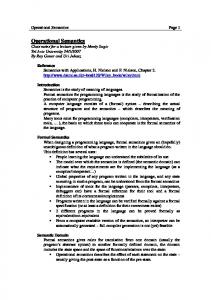
as a set of parameter values, and a specification, written in the notation, and produce a more primitive, equivalent form of the specification, such as a transition relation. The existing tool suite Fusion [20, 21] is a natural choice to implement our parameterized semantics-based model compiler Metro, because the input language, S+, for Fusion, a higher-order-logic language, is general and expressive for representing template definitions. In addition, the symbolic functional evaluation (SFE) [22] inside Fusion takes as input a description of a notation’s semantics embedded in logic and uses it to expand the meaning of an S+ specification into its transition relation. Fusion’s BDD-based model checker can then be used to analyze the transition relation. Figure 1.4 describes the structure of our parameterized model compiler Metro using a data flow diagram. We have codified the parameterized template definitions and the composition operators, expressed in logic and set theory, in higher-order functions. For example, there is a parameterized predicate that identifies the set of enabled transitions, and another parameterized predicate that updates a specification’s execution with the effects of an executing transition. These and similar functions and predicates implement the common semantics of model-based notations. Composition operators are defined as predicates over the execution semantics of the operator’s two components. We have implemented the composition operators as logic constraints that constrain which components are enabled and execute, and how the components exchange events and variables. The specification in notation M must be transformed into a CHTS. For most of the well-used model-based notations, this transformation is a transliteration, which is a simple mapping between the two notations’ syntactic constructs without involving any abstraction, flattening of composition, or semantics evaluation. The semantics of a notation M


13

Semantics of Notation M Given by Template-Parameter Values

user

Metro Common Template Semantics

Spec in Formal Notation M

Transliteration

Pre-defined Composition Operators

Template Defintions for Notation M

Spec in CHTS

Composition Operators for Notation M

Model Compiler (SFE) in Fusion

Transition Relation

True or False (with Counterexample)

Model Checker

Transliteration

in Fusion

SMV model

Model Checker SMV

Legend External Entity

Process

Data Flow

Data Store

Figure 1.4: Parameterized model compiler


14

is expressed by a set of template-parameter values, which apply to all HTSs in the specification, and by a set of composition operators, which are either pre-defined composition primitives or new composition operators. In Metro, SFE takes as input all of these definitions in S+, symbolically evaluates and expands the specification, and produces as output the specification’s transition relation, which can be checked by Fusion’s symbolic model checker. The transition relation can also be transliterated into the input languages of existing model checkers, such as SMV. If a model-based notation changes its syntax constructs, the transliteration into an HTS specification needs to be revised with no change to its template-semantics description. It is also possible that changes to a notation’s syntax cause changes to its semantics, in which case the template-parameter values need to be revised to reflect the changes. The template semantics for model-based notations simplifies the expression of notations’ semantics, therefore, the effort required for mapping a new notation or a notation variant to analysis tools is reduced by using our parameterized model compiler. To make the better use of well-established model checkers, such as SMV [65] and NuSMV [15] whose performance has been optimized, Lu et.al. [44, 45] developed a templatesemantics-based translator from model-based notations directly into the input language of the SMV family of model checkers. The translator, called Express (Figure 1.5), takes as input a specification, the semantics description of the specification notation expressed as template parameters, and produces an SMV model of the specification. This parameterized translator supports a fixed set of parameter values and pre-defined composition operators, so it can be used to check specifications written in many different existing model-based notations and variations of those notations. These notations’ semantics are defined by


15

simply selecting a combination of parameter values and using the composition operators that Express provides.

Template Parameter Values

Specification in CHTS

input

Express output

input

Hard-coded Template-Semantics Definitions

Specification in SMV’s input lang.

Figure 1.5: Express: Parameterized translator In Express, the template semantics is hard-coded, and the template-parameter values and composition operators that Express supports are fixed. Therefore, the translator needs to be revised, that is, the translation of new parameter values and new composition operators have to be implemented, to accommodate new parameter values or new composition operators. In contrast, in Metro, the common semantics, parameterized by user-provided parameter values and composition operators, are embedded in higher-order logic. Whenever a notation’s semantics changes or a new notation is introduced, only the template-parameter values need to be revised to reflect the changes rather than modifying Metro itself. Express translates specifications into the well-established model checker SMV, which provides more efficient analysis than Fusion’s model checker. However, the SMV model produced by Express is highly stylized and structured to support the easy introduction of new template-parameter values. As such, Express’s output is less suitable


16

to be transformed to the input languages of other analysis tools. Metro produces a transition relation in logic, a more primitive form of specification, which can be transliterated to other tools.

1.3

Contributions

The dissertation proposes a new template-based approach to structure the operational semantics of a model-based notation. Template semantics is a useful, parsable input language for parameterized model compilation, which can compile specifications in multiple notations. We implement a parameterized model compiler based on template semantics. The model compiler can compile a CHTS specification and its template-semantics description into a transition relation expressed in logic, which can be checked by a symbolic model checker. A parameterized model compiler eases the translation of new notations or notation variants to analysis tools. The model compiler does not need to be reconstructed whenever the notation’s semantics evolves; rather, users need modify only the parameter values or define new composition operators to reflect the notation’s changes. We use template semantics to document most of the semantics of ten existing modelbased notations, BTSs [47], CSP [37], CCS [51], LOTOS [40], Harel’s original statecharts [32], STATEMATE [33], RSML [43], SCR [35], SDL [41], and Petri Nets [52, 58]. The key feature of template semantics is its separation of concerns among aspects of notations’ semantics: the common execution semantics are pre-defined as a template of parameterized definitions; notation-specific behaviours are defined by the user in the form

1.4. THESIS VALIDATION

17

of parameter values; and composition operators are defined separately as parameterized constraints on the ways in which components execute and share information. This separation makes template semantics easy to understand and to parse in that it is possible to consider individual aspects of the semantics mostly in isolation from each other and a user’s input is relatively small.

1.4

Thesis Validation

The thesis was validated as follows. We developed template semantics by attempting to capture the common semantics of the seven model-based notations of our initial survey list. In doing so, we considered not only the effects of these seven notations on the template definitions, but we also tried to hypothesize new and synthesized variants of these notations, and to consider how the variants would be expressed using the template. We show that template semantics can be used to describe succinctly a variety of notations and it is particularly well-suited to notations with control states and events – the semantics of such a notation is represented as a set of parameter values, each of which is a simple and small logic formula on the order of less than ten primitives, plus a set of selected composition operators provided in the template. Template semantics’ approach of structuring notations’ execution semantics into template definitions that are parameterized by a set of smaller and simpler template-parameter expressions makes it easier to document the semantics of notations. Because the template parameters focus on differences among notations, we demonstrate that template seman-


18

tics can be used to compare notation variants, such as statecharts variants (Harel’s original statecharts [32], Maggiolo-Schettini et.al.’s statecharts [46], RSML [43], STATEMATE [33], and UML state models [56]). The main goal of this work is to provide a framework for constructing a semantics-based model compiler to facilitate the mapping of different notations to analysis tools. We have implemented a parameterized model compiler, which is a program that takes the templatesemantics description of a notation and compiles a specification in the notation into an underlying primitive representation that can be checked using model checkers. We use specifications of a heating system and a single-lane-bridge system as two examples to show that template semantics is a parsable input language to the parameterized model compiler. We demonstrate that using template semantics, multiple notations can be compiled by the same parameterized model compiler. This approach is verified by using model checking to show that the transition relation produced by the model compiler preserves certain properties of the original specification. The correctness of template semantics is validated by model checking two case studies with both a hand-generated SMV model and an SMV model generated using the templatesemantics-based tool, Express. We show that both models satisfy the same set of properties. In addition, the creation of Express shows that template semantics can be used to construct different types of model compilation to facilitate the mapping of multiple notations to analysis tools.

1.5. OVERVIEW OF DISSERTATION

1.5

19

Overview of Dissertation

This rest of the dissertation is organized as follows. Chapter 2 discusses related work. Chapter 3 presents the basic computation model, hierarchical transition systems, behind template semantics and presents our template for defining notations in terms of HTSs. In Chapter 4, we use template parameters to define a set of composition operators. Chapter 5 outlines our template-semantics-based parameterized method for model compilation and discusses the implementation of the parameterized model compiler. In Chapter 6, we evaluate the parameterized model compiler on two case studies, which are specified in different notations and exercise a broad range of composition operators, and show that template semantics can express the semantics of multiple model-based notations. We summarize and conclude in Chapter 7.

Chapter 2 Related Work This chapter discusses related work on automated analysis of model-based specifications. There are many well-established methods and tools for automatically verifying specifications written in model-based notations: an analyzer can be customized for a particular notation, a translator can be written from the notation to the input languages of one or more existing analyzers, or a semantics-based approach can be developed to map a notation to analysis tools automatically from the description of the notation’s semantics. Formalizing the semantics of specification notations is a first step towards mapping notations to analysis tools. We examine these different approaches in the following sections.

2.1

Semantics of Model-Based Notations

There has been substantial related work on formalizing the semantics of individual specification notations, such as defining the operational semantics of SDL [27], STATEMATE [33]

21

CHAPTER 2. RELATED WORK

22

and LOTOS [40]. An operational semantics describes the meaning of a notation by specifying how it executes on an abstract machine [69]. In other words, an operational semantics computes a system’s possible next execution steps using a set of semantics rules. Usually, the purpose of such work is to document a language’s precise semantics, possibly as a first step towards developing reasoning and verification tools. Such formalizations tend to be language-specific, making it difficult to compare the formal semantics of different languages and to generalize the semantics to accommodate multiple languages. There has been work on informally classifying the semantics of specification languages, (e.g., [14, 68]), the most famous of which is von der Beeck’s comparison of statecharts variants [67]. In von der Beeck’s work, many existing statecharts dialects are compared based on 19 criteria concerning the execution semantics of statecharts notations, e.g., instantaneous states, causality, and durability of events. These issues cover almost all aspects in which statecharts variants differ from each other. Wieringa [68] discusses different aspects of the execution semantics of state-transition diagrams, and Chou [14] describes the semantics of different composition and communication operators. Compared to these works, our template semantics is a more formal definition of a more fine-grained classification of semantics, expressed as a set of parameters, i.e., states, events, and variables as orthogonal factors. The catalogues of composition operators (parallel, interleaving, etc.) and communication operators (synchronous, asynchronous, etc.) identified in [14] and [67] are similar to ours, but we go further and define formally how each operator affects a model’s behaviour. To the best of our knowledge, there has been no comparable attempt to classify formally the step-semantics and composition semantics for model-based notations. We also express

2.2. AUTOMATED ANALYSIS OF MODEL-BASED NOTATIONS

23

variations in step-semantics as parameters, which makes it easier to define new notations and to identify both major and subtle differences among notations’ semantics.

2.2

Automated Analysis of Model-Based Notations

There are many analysis tools developed for automated checking of specifications written in particular model-based notations, such as Concurrency Workbench [17] and STATEMATE [33]. The Concurrency Workbench is a verification tool set customized for the CCS notation. The tool set transforms a CCS model into a labelled-transition system and provides different types of analyses. The equivalence-checking and preorder-checking tools examine if there are bisimulation relations between two labelled-transition systems. The model-checking tool determines if certain μ-calculus properties hold in a labelled-transition system. STATEMATE is a commercial tool suite for verifying statecharts models. STATEMATE provides tools for simulation and consistency checking of statecharts specifications. Algorithms for analyzing a model-based specification are very similar in their core: they compute the possible previous or next states to explore exhaustively a specification’s reachable state space. Because a customized analyzer is finely tuned for a certain notation, e.g., algorithms are optimized for the notation’s constructs and composition operators, it is usually more efficient than a general-purpose tool. However, to analyze specifications using customized analysis tools, analysis tools would need to be written for each notation and rewritten whenever the notation’s semantics evolves.


24

2.3

Translation from Notations to Analysis Tools

To reuse existing analysis tools to verify a specification, researchers developed translation approaches to map notations to the input languages of analysis tools without having to manually rewrite the specification in the input languages for those tools.

2.3.1

Translation Between Two Notations

Atlee and Gannon [1] developed a translator from SCR to the input language of the MCB model checker [10], so that an SCR specification’s safety properties and liveness properties specified in Computational Tree Logic (CTL) [16] could be verified. Chan et.al. [12] developed a translator from the RSML notation [43] to the input language of the SMV model checker [48]. A number of researchers have proposed translating specification notations into more fundamental modelling notations, such as first-order logic [70, 71], hierarchical state machines [50], labelled-transition systems [6], and hybrid automata [2]. Such notations are general enough to represent a variety of specification notations and can even accommodate specifications written in multiple notations. The verification tools and techniques associated with the target notation can be applied to the translated specification. People are familiar with the well-defined fundamental notations, so that the effort required for the translation could be eased. However, translating into these notations may not preserve the structure of an original specification. Cheng and her group [8, 13, 49] have done intensive research on formalizing and translating Object Modelling Technique (OMT) [64] and UML models into formal notations,

2.3. TRANSLATION FROM NOTATIONS TO ANALYSIS TOOLS

25

such as LOTOS and Promela (the input language to SPIN [38]). They have developed automated frameworks based on sets of rules, which encode both the syntactic and semantic mapping, to transform the syntactic constructs, e.g., states and events, of the source notations to the syntactic constructs, e.g., processes and gates in LOTOS, of the target notations. The advantages of this rule-based translation approach are that it simplifies the translation process by separating concerns, it enables reuse, and it keeps the structure of an original specification. Cheng et.al. [13] have used this work to facilitate the integration of specifications comprising three different OMT models (object, functional, and dynamic models). Translation is a heavy process that transforms both the syntax and semantics of a notation into the form of the target notation. As a notation evolves, the translator is hard to change because semantics changes. Changes to the semantics of composition operators may affect multiple translation rules and may be dispersed in many modules in the translator.

2.3.2

Intermediate Languages

To reduce the number of translators from notations to the input languages of analyzers, researchers have introduced intermediate languages, such as SAL [3], IF [9], Action Language [11], Bandera Intermediate Representation (BIR) [19], OMML [30], and CDL [42]. These intermediate languages are designed to be elegant yet expressive target languages that ease translations between notations. In most of these cases, there exist translators that map from several specification notations to the intermediate language, and there are translators that map to and from the intermediate language and the input languages of


26 verification tools.

SAL is designed as an intermediate language, such that different languages (e.g., Java and Verilog) can be translated to it. SAL has been translated to PVS and SMV. SDL and LOTOS are intended input languages for the intermediate language IF. IF has been mapped to different tools, such as the SPIN model checker [38]. CDL is the intermediate language developed for the VeriTech project, which aims at easing the translation between the input languages of SMV, SPIN, Murphi, etc. BIR is an intermediate notation for Java programs, and has been translated to the input languages of PVS, SMV, and SPIN. RSML and SCR can be translated to Action Language, which can be analyzed using the connected model checker at the back-end. OMML [30] is an XML-based language, established for representing different requirements-specification languages. Translators between SCR and OMML and between P-EBF [29] and OMML have been developed. Intermediate languages usually are designed to be expressive for not only their target notations, but also notations that have similar features. These intermediate-language approaches allow the specifications to be analyzed using multiple verification tools. Bogor [63] is a parameterized model-checking framework. Borgor is developed to construct domain-specific (for different software artifacts, such as designs and code) model checkers using its well-defined, easily-extended, model-checking-algorithm modules and optimization modules. The Bogor framework provides an architecture as a guideline for constructing optimized model checkers. Different from other translators we mentioned, Bogor is a parameterized back-end framework, which produces for the intermediate language BIR customized model checkers by choosing options of the modules. Intermediate-language approaches reduce the number of translators between specifi-

2.4. SEMANTICS-BASED APPROACHES

27

cation notations and analysis tools. However, intermediate languages solve none of the problems of the translation approach: a translator needs to be built for each specification notation and needs to be continuously modified as the notation’s semantics evolves.

2.4

Semantics-Based Approaches

More recently, to alleviate problems of translation, researchers have been working towards semantics-based mapping from notations to analysis tools, using the descriptions of notations’ semantics as input. This approach is the goal of the work of Day and Joyce [22], Pezzè and Young [59, 60], and Dillon and Stirewalt [24, 23, 66].

2.4.1

Fusion

Day and Joyce [22] embed the semantics of a notation in higher-order logic and automatically compile a next-state relation for a specification using symbolic functional evaluation (SFE) of the notation’s semantics definitions. Embedding avoids the translation step and the effort to construct and maintain translators because embedding represents the semantics of a notation in logic rather than hard-coding the semantics in a translator. Thus, to change the semantics, the user needs to change only the input data rather than the implemented tool. SFE expands a specification’s definitions and its semantics definitions into a transition relation that refers only to built-in constants, e.g., “∧” and “∨”, in higher-order logic. After an abstraction step (if necessary) on the transition relation, various automatedanalysis methods, such as completeness and consistent checking and model checking, can be applied to verify the specification. The advantage of Fusion is that it is fully automated.


28

Notations have also been embedded in the theorem prover PVS [57], and PVS’s model checker has been used to analyze these specifications.

2.4.2

Hypergraph

Pezzè and Young [59, 60] embed the semantics of model-based notations into hypergraph rules, which specify how enabled transitions are selected and how executing transitions affect the specification’s hypergraph model. A hypergraph, a Petri-Nets-like notation, represents the execution semantics of a model-based notation using three different types of hypergraph rules: enabling rules, matching rules, and firing rules. Enabling rules determine the set of enabled transitions; matching rules find subsets of transitions, at most one from each component, that are mutually compatible to execute together; and firing rules determine the next state, based on the effects of the executing transitions. A state-space analyzer for a notation can be constructed based on the notation’s semantics in hypergraph rules. A manual transformation takes as input a specification in a model-based notation and produces an internal representation of the given specification in terms of hypergraphs. Various state-space analysis techniques, such as simulation and reachability analysis, can be applied to check hypergragh specifications. A hypergraph model defines not only the execution semantics of components written in a particular specification notation but also the semantics of the composition of components specified in different notations, e.g., the composition of a Petri Net and an Ada task. Each component uses its own enabling and firing rules to determine the execution step and the next state. The composition of two components, described using matching rules, constrains which transitions from the two components may execute concurrently. Thus,

2.4. SEMANTICS-BASED APPROACHES

29

the hypergraph enabling rules and firing rules are similar to our pre-defined template definitions for enabling conditions and post-conditions, respectively; and the matching rules are similar to our composition operators’ definitions. But our template definitions are parameterized by a set of smaller parameter definitions, and our composition operators are defined separately as predicate constraints. The hypergraph approach is limited to statespace exploration analysis, e.g., generating reachability graphs, of specifications without variables, and the transformation from a specification into an internal representation (hypergraph) is not automated. Our parameterized model compiler Metro is implemented to transform automatically a specification into a transition relation, which can be checked by model checkers.

2.4.3

Amalia

Dillon and Stirewalt [24, 23, 66] propose an approach called Amalia for mapping the structural-operational-semantics [61] description for a specification notation, e.g., process algebra and temporal-logic notations, to a tool called a step analyzer. The user defines the structural operational semantics for a notation, and semi-automatically translates the semantics description into a step analyzer. The step analyzer accepts a specification in that notation and generates for the specification an inference graph, which is a data structure that determines the possible next steps. The step analyzer uses this inference graph to calculate all of the specification’s possible next steps, expressed as specifications, which in turn can be fed back into their tool to produce their respective inference graphs. Exhaustively repeating this process explores the specification’s state-space. Similarly, Cleaveland and Sims [18] have incorporated a Process Algebra Compiler


30

(PAC) into the front-end of the Concurrency Workbench [17]. PAC takes as input the abstract syntax of a process algebra and its semantics description in structural-operationalsemantics rules, and produces a state-space analyzer. The state-space analyzer can accept a process-algebra specification and generate an internal representation that can be input to Concurrency Workbench, a verification tool suite for the CCS notation.

2.5

Summary

In this chapter, we examined existing approaches for writing analysis tools or translators for particular notations, and mapping specification notations to analysis tools from descriptions of the notations’ semantics. A translator or a customized analysis tool for a notation can be efficient and fully automated, but needs to be revised whenever the notation evolves. Semantics-based approaches can alleviate this problem, however, the semantics of a notation is complex and formalizing it in a semantics-description language, such as higher-order logic or hypergraph rules, is challenging.

Chapter 3 Hierarchical Transition Systems (HTSs) In this chapter, we introduce hierarchical transition systems (HTS) as template-semantics’ computation model for model-based notations. An HTS is a hierarchical, extended finitestate machine with no concurrency – in statecharts terminology, an HTS supports ORstate hierarchy but not AND-state hierarchy. Its syntax is adapted from basic transition systems [47] and statecharts [31], and its semantics is parameterized. Concurrency is introduced by the composition operators, which are defined in the next chapter.

3.1

Syntax of HTSs

We present the syntax of HTSs in this section, along with functions for accessing parts of an HTS.

31

32

CHAPTER 3. HIERARCHICAL TRANSITION SYSTEMS (HTSS)

DEFINITION 3.1 (HTS Syntax) A hierarchical transition system (HTS) is an 8-tuple, S , S I , S F , S H , E , V , V I , T , where • S is a finite set of control states. Each state s ∈ S is either a super-state, which contains other states, or a basic state, which contains no other states. Each superstate has a unique default child state, which is entered if the super-state is the destination state of a transition. • S I is a predicate describing multiple possible initial sets of control states. • S F specifies the set of final basic states. No transition can exit a final state. • S H is a state hierarchy. It defines the partial ordering on states with respect to their ancestor super-states. Basic states are all maximal elements and there are no other maximal elements. There is a unique minimal element called the root state. • E is a finite set of events including both internal and external events. • V is a finite set of typed data variables. • V I is a predicate describing the possible initial values of the variables in V . • T is a finite set of transitions. We use the identifiers of the 8-tuple in definitions throughout the thesis to refer to their respective HTS elements. We assume that the names of states, events, and variables that are local to an HTS are unique within a specification.

3.1. SYNTAX OF HTSS

33

DEFINITION 3.2 (HTS Transition) Each transition in T has the form,

src

name: trig, [cond], ^gen, /asn, #prty

dest

where • src, dest ⊆ S are the transition’s sets of source and destination states, respectively. We use sets of sources and destinations to cover notations that allow transitions to have zero or multiple source or destination states. • name is the name of the transition. • trig ⊆ E are zero or more triggering events. • cond is a predicate over V . • gen ⊆ E are zero or more generated events (a transition may generate multiple events). • asn are a sequence of assignments to some data variables in V . • prty is the transition’s explicitly-defined priority. Depending on the notation, some transition elements may be optional.


34

We assume that a specification represented as an HTS conforms to its original notation’s well-formedness conditions. A typical well-formedness condition would be one that prohibits a transition from having multiple destination states or making multiple assignments to the same variable. Figure 3.1 shows an example HTS, in which S0, S1, S2, and S3 are super-states, and the others are basic states. The top state S0 is the root state of the HTS, and its default state is S1, as indicated by the small arrow pointing to S1.

S0 S1

S2

S3 S7 t4 S8

t5

t2

S5 S9

t1 t3

S4 S6

Figure 3.1: Example showing state hierarchy in an HTS Throughout the thesis, we use the helper functions described in Table 3.1 to access information about an HTS. The functions above the double line are accessor functions on transitions, whereas the functions below the double line are functions on states. All functions implicitly take an HTS as an argument. For example, the function ancest takes

3.1. SYNTAX OF HTSS

35

Function

Signature

Description

src(τ ) dest(τ ) trig(τ ) cond(τ ) gen(τ ) asn(τ ) prty(τ )

T T T T T T T

parent(s) children(s) type(s) default(s) ancest(s) entered(st)

S →S S → 2S S → {super , basic} S →S S → 2S 2S → 2S

scope(τ )

T →S

rank (s)

S →N

→ 2S → 2S → 2E → exp → 2E → 2[V ×exp ] →N

source states of transition τ destination states of transition τ events that trigger transition τ transition τ ’s predicate guard condition events generated by transition τ ’s actions variable-value assignments in transition τ ’s actions transition τ ’s priority value parent state of state s immediate child states of state s type of state s default state of state s ancestor states of state s states entered when a set of states st are entered, including all ancestor states of the states in st and all relevant descendants’ default states lowest common ancestor state of transition τ ’s source and destination states the distance between state s and the root state, rank (s) = rank (parent(s)) + 1 where rank (root) = 0

exp: represents an expression 2x : represents the power set of the set x N: represents the set of natural numbers Table 3.1: HTS accessor functions


36

as input a state and returns the set of its ancestor states. In Figure 3.1, the ancestor states of state S8 are {S0, S1, S3 }. The function entered takes a transition’s set of destination states and returns all of their ancestor states and the relevant descendants’ default states that are also entered1 . The destination set of states, defined by function dest, of transition t1 is {S2 }, and all of the states entered, when S2 is entered, are {S0, S2, S5 }, where S0 is the ancestor of S2, and S5 is the default state of S2. The scope of transition t4 is state S3 and the scope of transition t5 is state S1. The helper functions are defined for a single state (or a set of states in the case of the function entered ) and a single transition, but we will also apply them to sets of states and sets of transitions. When applied to a set of states or a set of transitions, the function is applied to each element of the set: functions that return a set of results will return a set of sets of results, one for each element in the argument; the functions that return a single result will return a set of results.

3.2

Semantics of HTSs

We define the semantics of an HTS as a snapshot relation. A snapshot is an observable point in an HTS’s execution, and a snapshot relation relates two snapshots ss and ss if the system can move from ss to ss in a step. We define two types of steps between snapshots: a micro-step is the execution of a single transition, and a macro-step is a sequence of zero or more micro-steps. Our definitions for micro-step and macro-step are parameterized with notation-specific parameter predicates and parameter functions whose 1

The definition of entered is not standard in the literature. We will use this definition throughout this thesis.

3.2. SEMANTICS OF HTSS

37

values reflect the semantics of a particular notation. In this section, we describe the semantics definitions that are common to all HTSs, and in Section 3.3, we describe the parameters used in these semantics definitions.

3.2.1

Snapshots

A snapshot stores information about the current status of an HTS. This information determines which transition is enabled. The snapshot contains information about several aspects of an HTS. These aspects are orthogonal to one another as regards the identification of a set of enabled transitions. This orthogonality allow us to separate the execution semantics into smaller concerns. DEFINITION 3.3 (Snapshot) A snapshot is formally defined as an 8-tuple CS , IE , AV , O, CSa , IEa , AVa , Ia , where, • CS is the set of current states (CS ⊆ S ). If s ∈ CS , then so are all of s’s ancestors. • IE is the set of current internal events (IE ⊆ E ). • AV stores current variable values. The set AV is a function that maps each data variable in V to its current value. • O is the current outputs to be communicated to concurrent components and to the environment (O ⊆ E ). • CSa , AVa , IEa and Ia are auxiliary elements that accumulate data about the states, the variable values, and the internal and external events, respectively, that were used or generated in past transitions.


38

The template parameters use the eight snapshot elements to derive the sets of enabling states (states that can trigger transitions in the current snapshot), of enabling variable values (variable values that are used when evaluating guard conditions of transitions in the current snapshot), and of enabling events (events that can trigger transitions in the current snapshot); these sets in turn determine the transitions that are enabled in the current snapshot, and we call such transitions enabled transitions. Most model-based notations use only a subset of the snapshot elements (e.g., some process algebras have no variables). The unused snapshot elements can be simply set to be empty sets2 . Throughout the thesis, we use notation ss.XX to refer to the value of snapshot element XX in snapshot ss: for example, ss.CS refers to the value of the CS element in snapshot ss. A specification in a model-based notation usually reacts to external inputs I , which may be external events (represented as I .ev ), variable-value assignments (represented as I .var ) , or both. I is not part of the snapshot because it lies outside of the system. Instead, the template parameters must record input events and data in the snapshot elements if the events and data will be used.

3.2.2

Micro-Step Semantics

The micro-step relation Nmicro (ss, τ, ss ) means that the HTS can move from snapshot ss to a next snapshot ss by executing transition τ . Because an HTS is non-concurrent, only 2

In practise, unused elements are removed from the snapshot so that they do not affect the state space of the model in analysis.


39

one transition can execute in a micro-step.

DEFINITION 3.4 (Micro-Step) Nmicro (ss, τ, ss ) ≡ (τ ∈ pri enabled trans(ss, T )) ∧ apply(ss, τ, ss ) Predicate Nmicro (ss, τ, ss ) is satisfied if τ is an enabled transition of the highest relative priority and ss is the snapshot resulting from applying the effects of τ in ss. Nmicro is defined in terms of two definitions, pri enabled trans and apply, which are common to all notations.

DEFINITION 3.5 (Priority-Enabled Transitions) pri enabled trans(ss, T ) ≡ pri ({τ ∈ T | en states(ss, τ ) ∧ en events(ss, τ ) ∧ en cond (ss, τ )}) Function pri enabled trans(ss) returns a subset of an HTS’s transition set T that are enabled and have the highest relative priority, and we call such a subset the set of priorityenabled transitions, where • Template parameter pri is a function that finds the maximal subset of enabled transitions with the highest relative priority. If pri returns a set with more than one transition, then any of these transitions can be taken in a micro-step, meaning that the specification is nondeterministic. pri is a user-provided template parameter and is described in more detail in Section 3.3.

40

CHAPTER 3. HIERARCHICAL TRANSITION SYSTEMS (HTSS) • Template parameters en states, en events, and en cond are predicates that specify when a transition τ is enabled with respect to its source state(s), its triggering event(s), and its enabling condition, respectively. These predicates are user-provided template parameters that are defined in terms of the snapshot elements. Different notations make different decisions about which states, events, and variable values can trigger transitions and when. Possible values for these parameter predicates are described in Section 3.3. • The set {τ ∈ T | en states(ss, τ ) ∧ en events(ss, τ ) ∧ en cond(ss, τ )} is the subset of an HTS’s transition set T that contains enabled-transitions in a snapshot ss.

DEFINITION 3.6 (Apply) apply(ss, τ, ss ) ≡ let CS , IE , AV , O , CSa , IEa , AVa , Ia ≡ ss next CS (ss, τ, CS ) ∧ next IE (ss, τ, IE )

in

∧ next CSa (ss, τ, CSa ) ∧ next IEa (ss, τ, IEa )

∧ next AV (ss, τ, AV ) ∧ next AVa (ss, τ, AVa ) ∧ next O(ss, τ, O )

∧ next Ia (ss, τ, Ia )

Predicate apply constrains the possible next snapshot ss based on a current snapshot ss and the actions of executing transition τ . Predicate apply works by calling on user-provided template parameters next XX , which specify how each snapshot element is updated when a transition executes, according to the notation’s semantics. These template parameters are described in Section 3.3.


3.2.3

41

Macro-Step Semantics

A notation’s step-semantics is its macro-step semantics, which defines how many microsteps an HTS executes in response to a set of external inputs, before sensing the next set of external inputs. External inputs I may be external events, variable-value assignments, or both. We have identified two macro-step semantics, which we call simple and stable. A simple macro-step is equal to at most one micro-step. A stable macro-step is a maximal sequence of micro-steps, such that the sequence ends only when there are no more enabled transitions. Stable macro-step semantics capture the synchrony hypothesis [5], which assumes that the system can always finish reacting to external input before the environment changes the inputs’ values. Both of our macro-step relations Nmacro are total, that is, for every snapshot ss, there is a next snapshot ss by executing a macro-step. A macro-step starts with the snapshot that ends the previous macro-step. We define function reset that removes from this snapshot accumulated information about transitions that executed in the previous macro-step (e.g., events generated).

DEFINITION 3.7 (Reset Snapshot) reset(ss, I ) ≡ reset CS (ss, I ), reset IE (ss, I ), reset AV (ss, I ), reset O(ss, I ), reset CSa (ss, I ), reset IEa (ss, I ), reset AVa (ss, I ), reset Ia (ss, I ) Function reset returns the initial snapshot of the macro-step, calling, for each snapshot element XX , a user-provided template parameter reset XX , which is a function that removes information about transitions that executed in the previous macro-step, as per the


42

notation’s semantics. Template parameters reset XX are described in more detail in Section 3.3. In simple macro-step semantics, an HTS takes at most one micro-step per macrostep in reaction to a set of external inputs I . Notations differ as to whether they favour taking an enabled transition over stuttering, i.e., taking no transitions. In a diligent [47] simple macro-step, an HTS takes a micro-step if a transition is enabled, and otherwise makes no change to the reset snapshot:

DEFINITION 3.8 (Diligent Macro-Step) diligent Nmacro (ss, I , ss ) ≡

let ss i = reset(ss, I ) in if (∃ τ . τ ∈ pri enabled trans(ss i , T )) then (∃ τ . Nmicro (ss i , τ, ss )) else (ss i = ss )

In nondiligent simple macro-steps, idle steps have the same priority as diligent steps:

DEFINITION 3.9 (Nondiligent Macro-Step) nondiligent Nmacro (ss, I , ss ) ≡

let ss i = reset(ss, I ) in (∃ τ . Nmicro (ss i , τ, ss )) ∨ (ss i = ss )


43

In stable macro-step semantics, a macro-step is a maximal sequence of micro-steps that execute in response to a single set of external inputs. A macro-step ends when no transitions are enabled in the current snapshot: DEFINITION 3.10 (Stable Snapshot) A snapshot with no enabled transitions is called a stable snapshot. stable(ss) ≡ pri enabled trans(ss, T ) = When a stable snapshot is reached, a new macro-step starts with a new set of external inputs I . Figure 3.2 depicts a macro-step of three micro-steps that execute three transitions t1, t2, t3, respectively. SS0 is the starting snapshot of the macro-step i.e., the stable snapshot of the last macro-step, and SS 3 is the stable snapshot marking the end of the macro-step. At the beginning of the macro-step, functions reset XX are called to initialize snapshot elements XX in SS0 with a set of inputs I : the results are recorded in SS0i. In the first micro-step, transition t1 is one of the priority-enabled-transitions in SS0i, so it is chosen to execute, and its actions are used to update snapshot SS0i to snapshot SS1. In the next micro-step, transition t2 executes and is used to update each snapshot element XX in SS1 to SS2.XX as showed in Figure 3.2. In the third micro-step, transition t3 executes and the HTS reaches the snapshot SS3, which is a stable snapshot, and the HTS is ready to sense a new set of inputs to start another macro-step. We formally define the stable macro-step semantics using a relation N k , which is true for a pair of snapshots if there is a sequence of k micro-steps from the first snapshot to the second.


44

N 0 (ss, ss ) ≡ (ss = ss ) N k +1 (ss, ss ) ≡ (∃ ss , τ . Nmicro (ss, τ, ss ) ∧ N k (ss , ss ))

DEFINITION 3.11 (Stable Macro-Step) stable A stable macro-step Nmacro (ss, ss ) is defined as a finite sequence of micro-steps, terminat-

ing in a stable snapshot ss . stable Nmacro (ss, I , ss ) ≡

let ss i = reset(ss, I ) in if ¬stable(ss i ) then (∃ k > 0 . N k (ss i , ss ) ∧ stable(ss )) else (ss i = ss ) This definition assumes ss is a stable snapshot.

Some notations, such as RSML [43], do not guarantee that there is a finite number of micro-steps that make up a macro-step. It is not possible to write a well-founded recursive definition that matches their semantics. In practise, an analyst, for the purpose of verifying a given specification, would not implement the above definition of a stable macro-step. Rather, the analyst would use the micro-step relation as the next-state relation for the system, and would check properties at the macro-step level by prepending the stable predicate as an antecedent to their properties; this is how macro-level properties were model checked against the RSML specification for TCAS II [12].


45

A macro-step A micro-step

Input (I) SS0

SS0i

reset_CS (SS0, I) reset_IE (SS0, I) reset_AV (SS0, I) reset_O (SS0, I) reset_CSa (SS0, I) reset_IEa (SS0, I) reset_AVa (SS0, I) reset_Ia (SS0, I)

t1

SS1

t2

SS2

next_CS (SS1, t2, SS2.CS) next_IE (SS1, t2, SS2.IE) next_AV (SS1, t2, SS2.AV) next_O (SS1, t2, SS2.O) next_CSa (SS1,t2,,SS2.CSa) next_IEa (SS1, t2, SS2.IEa) next_AVa (SS1,t2, SS2.AVa,) next_Ia(SS1, t2, SS2.Ia)

Figure 3.2: A stable macro-step of an HTS

t3

SS3


46

3.2.4

Initial Snapshots

An HTS starts executing from a set of possible initial snapshots ss I , whose definition is the same for all macro-step semantics.

DEFINITION 3.12 (Initial Snapshot) ss I ≡ { CS , , AV , , , , , | AV |= V I ∧ CS |= S I } V I and S I are predicates on the HTS’s initial sets of states and of variable assignments, respectively. The sets of internal events and output events are initially empty. This definition allows there to be multiple possible initial snapshots. In future sections, we use ss I to refer to a snapshot at the beginning of the system’s execution and ss i to refer to a reset snapshot at the beginning of a macro step.

3.3

Template Parameters

The six definitions Nmacro , Nmicro , reset, pri enabled trans, apply, and stable described above constitute the common semantics in our template. These definitions are parameterized by functions and predicates that, for a notation, specialize how to determine which transitions are enabled in a snapshot, how to select an enabled transition to execute, and how to calculate the effects of a transition’s actions on a snapshot. As such, these parameters capture the semantic differences among notations. The list of template parameters is provided in Table 3.2. The reset XX template parameters listed in the column labelled “Start of Macro-step” specify how the value of each

3.3. TEMPLATE PARAMETERS

47

snapshot element is updated at the beginning of every macro-step. Their main purpose is to clean out data accumulated in the previous macro-step, e.g., resetting the set of current internal events to be empty. The column labelled “Micro-step” lists template-parameter predicates next XX that specify how each snapshot element XX is updated by the actions of the executing transition in a micro-step. These predicates are passed the entire snapshot because they may refer to other snapshot elements. Primed arguments, e.g., CS , refer to values of snapshot elements in the next snapshot ss . Predicates en states, en events, and en cond specify which states, events, and variable values recorded in snapshot ss can be used to enable transitions. Parameter macro semantics specifies the type of macro-step semantics (simple or stable, and whether diligent transitions have priority over idle transitions in micro-steps). Parameter pri specifies a priority scheme over a set of transitions by defining the subset of highest-priority transitions. The template parameters are organized in Table 3.2 by language construct. For example, the seven event-related parameters work together to determine which events can enable transitions and how event information is updated: • reset IE, reset IEa , and reset Ia update IE , IEa , and Ia , respectively, with input I at the beginning of each macro-step. Their main purpose is to clean out event-related data accumulated in the previous macro-step, e.g., resetting the set of current internal events to be empty, and recording the environment’s input I in snapshot element Ia . • en events determines how event information in IE , IEa , and Ia is used to enable transitions. • next IE, next IEa , and next Ia determine how transition τ ’s actions affect the possi-

48

CHAPTER 3. HIERARCHICAL TRANSITION SYSTEMS (HTSS) Affected Snapshot Element states

events

variables outputs additional parameters

Start of Macro-step Micro-step reset CS(ss, I ) next CS(ss, τ, CS ) reset CSa (ss, I ) next CSa (ss, τ, CSa ) en states(ss, τ ) reset IE(ss, I ) next IE(ss, τ, IE ) reset IEa (ss, I ) next IEa (ss, τ, IEa ) reset Ia (ss, I ) next Ia (ss, τ, Ia ) en events(ss, τ ) reset AV(ss, I ) next AV(ss, τ, AV ) reset AVa (ss, I ) next AVa (ss, τ, AVa ) en cond(ss, τ ) reset O(ss, I ) next O(ss, τ, O ) macro semantics pri(Γ) : 2T

Table 3.2: Parameters to be provided by template user ble values for next current internal events (IE ), next auxiliary internal events (IEa ), and next recorded input events (Ia ). Similarly, the five state-related parameters work together to determine which states are active to enable transitions, and how the executing transition changes the state information in CS and CSa . The five variable-related parameters work together to indicate which variable values are used to evaluate enabling conditions of transitions, and how to update the variable values after a transition executes. The output-related parameters specify how to update the output after a transition executes. The following five subsections describe how a specifier can use these parameters to define the step-semantics for some popular notations. Tables 3.3–3.6 provide sample definitions. Abbreviation “n/a” means “not applicable”, in which case the predicate always returns


49

“true” and the function on the snapshot element is not used because the notation does not use that snapshot element.

3.3.1

States

In RSML and STATEMATE, a transition is enabled if its source states are a subset of the current states. These semantics allow infinite loops in a macro-step. Harel et al.’s [32] original formulation of statecharts avoids infinite loops by allowing each non-concurrent component, i.e., each HTS, to execute at most one transition per macro-step: the sequence of micro-steps that makes up a macro-step can execute multiple transitions, each of which is from a different HTS. We express this semantics by using snapshot element CS to maintain the set of current states, by using element CSa to maintain the set of enabling states, and by setting CSa to the empty set after the HTS takes a step, to disallow additional transitions from the same HTS in the current macro-step. We can envision an alternate state semantics that allows an HTS to take multiple micro-steps in a macro-step, and prevents infinite loops by prohibiting states being exited more than once in a macro-step.

Table 3.3 shows examples of definitions for the state-related template parameters. In the following, we describe some example values for the state-related template parameters. • reset CS (ss, I ) specifies the value of CS at the start of a new macro-step. This value depends on the current value of CS in snapshot ss (ss.CS ). Example values are ss.CS , meaning that the value of CS does not change at the start of a macro-step; and “n/a”, meaning that the notation has no concept of control states.


50

Parameter

statecharts [32]

reset CS(ss, I ) ≡

ss.CS

next CS(ss, τ, CS ) ≡ reset CSa (ss, I ) ≡ next

CSa (ss, τ, CSa )

en states(ss, τ ) ≡

RSML, STATEMATE

≡

CS = entered (dest(τ )) ss.CS

n/a

CSa

n/a

=

src(τ ) ⊆ ss.CSa

src(τ ) ⊆ ss.CS

Table 3.3: Sample definitions for state-related template parameters

• next CS (ss, τ, CS ) specifies how the value of snapshot element CS is updated to CS when transition τ executes. CS is affected by τ ’s destination states, dest(τ ), if the set of control states is not empty. Example values are CS = dest(τ ), meaning that the set of current states becomes the executing transition’s destination states dest(τ ); CS = entered (dest(τ )), meaning that the set of current states CS becomes the executing transition’s destination states dest(τ ), plus the destination states’ ancestor states and its descendants’ default states; and “n/a”, which means that the notation has no concept of control states. • reset CSa (ss, I ) specifies the value of CSa at the start of a new macro-step. Example values are ss.CS , meaning that the value of CSa is equal to the set of current states ss.CS at the start of the macro-step; and “n/a”, which means that the snapshot contains no extra state information. • next CSa (ss, τ, CSa ) specifies how the value of snapshot element CSa is updated to CSa when transition τ executes. Example values are CSa =

, meaning that the value

of CSa is empty after a transition executes, which means at most one transition in


51

an HTS can execute in a macro-step; and “n/a”, which means the snapshot contains no extra state information. • en states(ss, τ ) specifies which states stored in state-related snapshot elements (CS and CSa ) can trigger transitions. Different notations make different decisions about which states can trigger transitions and when. Parameter en states is a predicate that compares the source states of a transition τ with the values of the state-related snapshot elements in snapshot ss, and decides whether the snapshot’s state-related elements enable τ . Example predicates are src(τ ) ⊆ ss.CS , meaning that τ ’s source states must all be states stored in CS ; src(τ ) ⊆ ss.CSa , meaning that τ ’s source states must all be states stored in CSa ; and “n/a”, which means that the notation has no concept of states.

3.3.2

Events

Table 3.4 shows examples of definitions of event-related template parameters. These events can be internal and/or external events. Process algebras such as CCS use only external events. Statecharts-based notations have both internal and external events. For notations that differentiate syntactically between internal events and external events, we use intern ev (E ) to mean the set of internal events and extern ev (E ) for the set of external events. In STATEMATE and RSML, only internal events generated in the previous microstep can trigger a transition, whereas in the original statecharts semantics, internal events generated by transitions remain enabling events throughout the macro-step.


52 Parameter

CCS

reset IE(ss, I ) ≡

n/a

next IE(ss, τ, IE ) ≡

n/a

IE = ss.IE ∪ gen(τ )

reset IEa (ss, I ) ≡

n/a

n/a

n/a

n/a

≡ n/a

n/a

n/a

n/a

next

IEa (ss, τ, IEa )

statecharts [32]

reset Ia (ss, I ) ≡

RSML

STATEMATE

IE = gen(τ ) ∩ intern ev (E )

IE = gen(τ )

I .ev

next Ia (ss, τ, Ia ) ≡

true

en events(ss, τ ) ≡

trig(τ ) ⊆ ss.Ia

Ia = ss.Ia

Ia = trig(τ ) ⊆ ss.IE ∪ ss.Ia

reset O(ss, I ) ≡ O = ss.O ∪ next O(ss, τ, O ) ≡

O = gen(τ )

O = ss.O ∪ gen(τ )

(gen(τ ) ∩

O = gen(τ )

extern ev (E ))

Table 3.4: Sample definitions for event-related template parameters

In all statecharts variants, the external input events I .ev are enabling events at the start of each macro-step. In RSML and STATEMATE, external events can trigger transitions only in the first micro-step of a macro-step. In statecharts, external events remain enabling events throughout the macro-step. We can also imagine a notation in which an external event remains an enabling event until it triggers a transition or until the macro-step ends. Statecharts accumulate as output all of the events generated during the micro-step. RSML accumulates all of the generated external events. STATEMATE only considers as output the events generated in the last micro-step of the macro-step. In the following, we describe some example values for the event-related template parameters.


53

• reset IE (ss, I ) specifies the value of IE at the start of a new macro-step. Example values are

, which means that all previously generated events are discarded;

and “n/a”, which means that the notation has no concept of internal events. Because IE records the current internal events, it does not record events I .ev from the environment. • next IE (ss, τ, IE ) specifies how the value of snapshot element IE is updated to IE when transition τ executes. IE may be affected by the events that τ generates, gen(τ ). Example values are IE = ss.IE ∪ gen(τ ), meaning that, events generated by executing transition τ are added to the events already in IE and no events are removed; IE = gen(τ ) ∩ intern ev (E ), meaning that, only those events that are designated as internal events and that are generated by executing transition τ are present in IE , and all events previously in IE are discarded; and IE = gen(τ ), meaning that, only those events generated by executing transition τ are present in IE . The last option is used to specify that only events generated in the last step can trigger transitions in the next step. • reset IEa (ss, I ) specifies the value of IEa at the start of a new macro-step, when the system senses new events I .ev from the environment and prepares to react to them. Example values are

, meaning that IEa is reset to be empty at the start of every

macro-step (all previously accumulated event information is discarded); and “n/a”, which means that the snapshot contains no extra event information. • next IEa (ss, τ, IEa ) specifies how the value of snapshot element IEa is updated to IEa when transition τ executes. IEa may be affected by τ ’s generated events, gen(τ ).

54

CHAPTER 3. HIERARCHICAL TRANSITION SYSTEMS (HTSS) The value of IEa may also depend on values in the snapshot, e.g., ss.IEa . Example values are IEa = ss.IEa ∪ gen(τ ), which means that events generated by executing transition τ are added to the set of events already in IEa ; and “n/a”, which means that the snapshot contains no extra event information. • reset Ia (ss, I ) specifies the value of Ia at the start of a new macro-step, when the system senses new events I .ev from the environment and prepares to react to them. An example value is I .ev , which means that Ia is set to be the new events sensed from the environment (I .ev ) at the start of every macro-step and all previous input events are discarded. • next Ia (ss, τ, Ia ) specifies how the value of snapshot element Ia is updated to Ia when transition τ executes. Ia may be affected by the events that τ generates, gen(τ ), and may also depend on values in the current snapshot, e.g., ss.Ia . Example values are “true”, which means that the value of Ia in snapshot ss is not relevant; Ia = ss.Ia , which means that throughout the macro-step, Ia always keeps the external events from the start of the macro-step; and Ia =

, which means that the value of Ia is

always set to be empty. In the last case, external events can trigger only the first transition of a macro-step. • en events(ss, τ ) compares the triggering events of transition τ with the values of the snapshot elements in snapshot ss, and decides whether the snapshot’s event-related elements enable τ . Example predicates are trig(τ ) ⊆ ss.Ia , which means that τ ’s triggering events must all be events stored in Ia ; trig(τ ) ⊆ ss.Ia ∪ ss.IE , that is τ ’s triggering events must all be events stored in either Ia or IE ; and trig(τ ) ⊆


55

ss.Ia ∪ ss.IEa , which means τ ’s triggering events must all be events stored in either Ia or IEa . IEa is used in some notations to record extra event information to help derive enabling events, e.g., it is used in statecharts to record negated events, which are described in Chapter 6. Table 3.4 also shows how the outputs for a micro-step are determined. • reset O(ss, I ) specifies the value of O at the start of a new macro-step, when the system senses new events I .ev from the environment and prepares to react to them. An example value is

, which means that O is reset to be empty at the start of every

macro-step (previous output is discarded). • next O(ss, τ, O ) specifies how the value of snapshot element O is updated to O when transition τ executes. O may be affected by τ ’s generated events, gen(τ ). The value of O may also depend on values in the current snapshot, e.g., ss.O. Example values are O = gen(τ ), which means only those events generated by executing transition τ in the current micro-step are present in O and all events previously in O are discarded; O = ss.O ∪ gen(τ ), which means that events generated by executing transition τ are added to the events already in O; and O = ss.O ∪ (gen(τ ) ∩ extern ev (E )), which means that only those events that are generated by executing transition τ and that are designated as external events are added to the events already in O.

3.3.3

Variable Values

Table 3.5 shows examples of definitions for variable-related template parameters.


56

In most notations, transitions’ enabling conditions are evaluated with respect to the current variable values. In contrast, in the original statecharts semantics, conditions and expressions are evaluated with respect to variable values that hold at the start of the macro-step, except for expressions within a cr operator, which are evaluated with respect to the current variable assignments. Thus for statecharts, we use snapshot element AV to maintain the set of current variable values, and use element AVa to maintain the variable values from the start of the macro-step; and we evaluate enabling conditions and assignment expressions with respect to both snapshot elements. Variable values are updated by overriding current value assignments with the transition’s variable assignments using the function assign described in Table 3.5. In STATEMATE, if a transition makes multiple assignments on the same variable, only the last assignment to the variable has an effect. RSML and statecharts do not allow transitions to make multiple assignments to the same variable. Some notations, such as the SMV input language [48], allow variable assignments to refer to values that hold at the start of the next micro-step. Because the next AV parameter is a predicate that takes the next snapshot’s variable values as an argument, we can accommodate such forward-referencing semantics for notations. In the following, we describe some example values for the variable-related template parameters. • reset AV (ss, I ) specifies the value of AV at the start of a new macro-step, when the system senses new input variables from the environment. This value may depend on the current value of AV in snapshot ss (ss.AV ) and input variables (I .var ). An


Parameter

statecharts [32]

reset AV(ss, I ) ≡

RSML

STATEMATE

assign(ss.AV , I .var )

next AV(ss, τ, AV ) ≡ reset AVa (ss, I ) ≡ next

57

AVa (ss, τ, AVa )

en cond(ss.AV , τ ) ≡

≡

AV = assign(ss.AV ,

AV = assign(ss.AV , AV = assign(ss.AV ,

eval ((ss.AV , ss.AVa ), asn(τ ))) eval (ss.AV , asn(τ )))

eval (ss.AV , last(asn(τ ))))


n/a

AVa

n/a

= ss.AVa

ss.AV , ss.AVa |= cond(τ )

eval (ss.AV , a): eval ((ss.AV , ss.AVa ), a): assign(X , Y ):

ss.AV |= cond(τ )

evaluates assignments a using variable values in ss.AV evaluates assignments a using variable values in ss.AV and ss.AVa updates assignments X with assignments Y ; ignores assignments in Y to variables not in X

last(a):

chooses the last assignment to each variable in the sequence of assignments a

Table 3.5: Sample definitions for variable-related template parameters

58

CHAPTER 3. HIERARCHICAL TRANSITION SYSTEMS (HTSS) example value is assign(ss.AV , I .var ), which means that at the start of a macrostep, the environment variables in AV read values from the input variables I .var , and their previous values are discarded. • next AV (ss, τ, AV ) specifies how the value of snapshot element AV is updated to AV when transition τ executes. AV is affected by τ ’s actions, asn(τ ). Example values are AV = assign(ss.AV , eval (ss.AV , asn(τ ))), which means that AV is updated by the assignments in τ , asn(τ ), where the assignments are evaluated with respect to the values in the current snapshot ss (ss.AV ); AV = assign(ss.AV , eval ((ss.AV , ss.AVa ), asn(τ ))), which means AV is updated by the assignments in τ , where the assignments are evaluated with respect to values in either the snapshot element (ss.AV ) or the snapshot element ss.AVa ; and AV = assign(ss.AV , eval (ss.AV , last(asn(τ )))), which means AV is updated by the assignments in τ , which are evaluated with respect to the values in the current snapshot (ss.AV ), and if τ makes multiple assignments to the same variable, only the last assignment is considered. • reset AVa (ss, I ) specifies the value of AVa at the start of a new macro-step, when the system senses new input variables from the environment (I .var ). This value may depend on the current value of AV in snapshot ss (ss.AV ) and input variables (I .var ). Example values are assign(ss.AV , I .var ), meaning that at the start of a macro-step, the environment variables in AVa read values from the input variables I .var , and the other variables are set to be equal to variable values in ss.AV ; and “n/a”, which means that the snapshot contains no extra variable information.


59

• next AVa (ss, τ, AVa ) specifies how the value of snapshot element AVa is updated to AVa when transition τ executes. Example values are ss.AVa , meaning that throughout the macro-step, AVa always maintains the variable values from the start of the macro-step; and “n/a”, which means that the snapshot contains no extra variable information. • en cond (ss, τ ) specifies which variable values stored in variable-related snapshot elements (AV and AVa ) can be used to evaluate the guard conditions of transitions. The parameter predicate en cond (ss, τ ) computes the condition cond in τ using the values of the variable-related snapshot elements in snapshot ss, and decides whether the variable values enable τ (in which case, the cond evaluates to “true”). Example values are ss.AV |= cond (τ ), meaning that the guard condition of τ is evaluated using variable values stored in AV ; ss.AV , ss.AVa |= cond (τ ), which means that the condition of τ is evaluated using the variable values stored in both AV and AVa (all the conditions will be evaluated to the variables values in AVa , except expressions within a cr operator); and “n/a”, which means that the snapshot contains no extra variable information.

3.3.4

Priority

Table 3.6 shows examples of definitions for template parameter pri , which returns the subset of transitions of highest priority. STATEMATE prioritizes transitions by the ranks of their scope, where rank and scope are described in Table 3.1 on page 35. The priority of transition t2 in Figure 3.1 on page 34 is the rank of scope(t2)= S1, which is 1. Lower-


60

ranked scopes have priority over higher-ranked scopes, which means that super-state behaviour is favoured over sub-state behaviour. UML[56] prioritizes transitions by the ranks of their source states. In this case, the priority of transition t2 is the rank of src(t2)= S3, which is 2. Transitions with higher-ranked source states have priority over transitions with lower-ranked source states, which means that sub-state behaviour overrides super-state behaviour.

Parameter STATEMATE pri(Γ) ≡

{τ ∈ Γ | ∀ t ∈ Γ. rank (scope(τ )) ≤ rank (scope(t))}

UML [56] {τ ∈ Γ | ∀ t ∈ Γ. rank (src(τ )) ≥ rank (src(t))}

Table 3.6: Sample definitions for priority template parameter

3.4

Summary

This chapter defines the syntax and the semantics of an HTS. We present three different macro-step semantics that are parameterized by 21 template parameters. We describe these parameters and their possible values in detail. These template parameters and another template parameter, resolve, are used in Chapter 4 to help define the semantics of composition operators.

Chapter 4 Composition Operators In this chapter, we describe the template semantics of a number of widely-used composition operators found in process algebras, statecharts variants, basic transition systems (BTSs), and SDL. Process algebras have a simple step semantics but a rich collection of composition operators, e.g., interleaving, rendezvous, choice. Statecharts have only two composition operators (parallel and interrupt), but they have more complex step semantics.

4.1

General Aspects of Composing Components

In template semantics, a composition operator specifies how multiple HTSs execute concurrently. The operands of a composition operator are components, where a component is either a basic component, i.e., an HTS, or a collection of components, i.e., composed HTSs (CHTS), that have been composed via some composition operator(s). We define our composition operators by specifying how the components’ snapshots change when the

61

CHAPTER 4. COMPOSITION OPERATORS

62

components take a step. The template-parameter values are common for all HTSs in a specification and are used by composition operators to ensure that their definitions are consistent with the specification’s execution semantics. Composition operators are represented as constraints on how to override the components’ snapshot relations, rather than as a new machine that would enumerate the sets of transitions (at most one transition for each HTS in each set) that can execute together. Using this approach the structure of the composition is not lost. Therefore, abstraction techniques such as partial-order reduction [26] can examine the basic components.

4.1.1

Composition Hierarchy

In template semantics, multiple HTSs are combined into a composition hierarchy via a collection of composition operators. Because all composition operators are binary, the composition hierarchy is a binary tree. Figure 4.1 shows an example of a composition hierarchy for a specification, which includes five basic components (HTSs) as leaves and four composed components as nonleaf nodes. HTS1 and HTS2 are composed into a component com2 by composition operator op2 ; HTS4 and HTS5 are composed into a component com4 by composition operator op4 ; HTS3 and com4 are composed by composition operator op3 into com3 ; and finally com2 and com3 are combined into a system (component com1 ) by op1. Because each HTS has its own set of transitions, the sets of transitions of a specification is also a tree structure that matches the composition hierarchy. Figure 4.2 presents an example specification for component com3 in the above composition hierarchy, where the dashed line is a composition, whose operator is named in the line’s center circle, and whose two operands are the boxes that lie on either side of the line.

4.1. GENERAL ASPECTS OF COMPOSING COMPONENTS

63

com1 op1 com2

com3

op2

op3

HTS1

com4

HTS3

HTS2

op4

HTS4

HTS5

Figure 4.1: An example composition tree

com3 HTS3 s1

com4 HTS4 s5

t1: a s2

t2: /y:=0

op3

t3: a

s3

s4

op4

t4: [x=1], ^b t5: d

Figure 4.2: An example CHTS

HTS5 t6: â s6

s7 t7: c


64

4.1.2

Snapshot Hierarchy

Each HTS has a local snapshot. For a specification that contains more than one HTS, the specification’s snapshots are organized into a tree structure matching the composition hierarchy of that specification. Figure 4.3 shows a snapshot tree for the example specification in Figure 4.2. A snapshot tree ss com3 for component com3 in Figure 4.1 includes two snapshot subtrees ss3 and ss com4, for HTS3 and com4, respectively, where ss3 is a leaf node, and ss com4 includes two snapshot subtrees (snapshot leaves) ss4 and ss5, for HTS4 and HTS5, respectively. ss_com3 op3

ss3

ss_com4

CS={s1} AV={(y,1)} IE={a} O= Ia={d}

op4

ss4

ss5

CS={s3} AV={(x,1)} IE={a,b} O={b} Ia={d}

CS={s7} AV= IE={a,b} O={a} Ia={d}

Figure 4.3: A snapshot tree for component com3 In defining the semantics of composition operators, we use vector notation ss, to rep−−−−→ resent a snapshot tree. Notation ss.XX refers to a tree of snapshot elements XX within

4.1. GENERAL ASPECTS OF COMPOSING COMPONENTS

65

a given snapshot tree ss, where each leaf is the snapshot element XX in an HTS’s snap−−−−−−−−→ shot. For example, ss com3.CS is a tree of snapshot elements CS , which includes ss3.CS , ss4.CS , and ss5.CS as leaves. We overload the notation

to mean an empty set or an empty tree. Two snapshot

trees are equal if their corresponding leaf snapshots are equal, and we compare snapshot trees only if they have corresponding composition hierarchies. The helper functions from Table 3.1 are also generalized to apply to trees of transitions and trees of states. For example, function gen(τ ) returns a tree of sets of generated events , where each leaf set of events Ev (can be Ev

) is generated by a leaf transition τ of the

tree τ , respectively. In Figure 4.2, gen(τ4 ), where the tree of transitions τ4 contains two leaf transitions t4 and t6, returns two sets of generated events {b} and {a} that forms a . tree of event sets Ev To override its components’ micro-step or macro-step semantics, a composition operator applies template parameter predicates reset XX and next XX thereby resetting and updating the components’ snapshot elements (this is described in detail in section 4.3). When applied to trees of snapshots and to trees of transitions, the template parameters, −−−−→ τ , ss .XX ), define how snapshot elements XX in corresponding leaf snapshots next XX (ss, in ss change values due to the execution of the transitions in the transition tree τ . Sim I ), define how snapshot elements XX clean ilarly, the parameter functions, reset XX (ss, up information about transitions that executed in the last macro-step and add information from the input I in the leaf snapshots in the snapshot tree ss.


66

4.1.3

Initial Snapshots

In all cases, except interrupt composition, the initial snapshot tree for the composed ma−→ −→ −→ chine comprises the component machines’ initial snapshot trees (ss I = (ss1I , ss2I )). We assume that initial values of shared variables are consistent among components.

4.2

Micro-Step Composition Semantics

We define micro-step composition operators as parameterized, composite relations that relate pairs of consecutive snapshot trees. For example, the composite micro-step relation for an operator op that composes two components component1 and component2 is op Nmicro ((ss 1 , ss 2 ), (τ1 , τ2 ), (ss 1 , ss 2 )).

2 for the two components It takes as arguments the two current snapshot trees ss 1 and ss component1 and component2, respectively; two trees of transitions, from component1 and component2, respectively; and the two next snapshot trees. The composite micro-step describes the relations between snapshot trees ss 1 and ss 1 , and between ss 2 and ss 2 , when component1 and component2 execute their respective transition trees τ1 and τ2 in the same micro-step. op The step semantics of each composition operator, Nmicro , is based on the micro-step 1 2 semantics of the two components, which we will call, Nmicro and Nmicro . The components’

micro-step semantics are defined in terms of each component’s composite operator (if it is a composed component) or its HTS semantics (if it is a leaf component). For example, the semantics for composition operator op4, which composes HTS4 and HTS5 (Figure 4.1),

4.2. MICRO-STEP COMPOSITION SEMANTICS

67

is defined by the step semantics for HTS4 and for HTS5, and plus constraints on how to overwrite HTS4 ’s snapshot and HTS5 ’s snapshot as appropriate for the composition operator. Each composition operator specifies when its components execute, how the changes in each component are shared, and when transfer of control from one component to another can occur. The operator must ensure that assignments to shared variables made by any component machine are reflected in all appropriate snapshots. In addition, the composition operator is responsible for “message passing” among components, making events generated by one component visible to the other component, either for the current step, e.g., rendezvous, or the next step. We use a set of macro definitions to facilitate the specification of the transfer of control and the exchange of variables and events in definitions of composition operators. We explain these definitions in the following subsections.

4.2.1

Substitution

A composition operator uses substitution to override its components’ behaviour: that is, to override the assignments to snapshot elements of their components’ micro-steps or macro-steps. For example, the sequence composition operator wipes out a component’s states when control is transferred out of the component. We represent the override of an assignment using substitution notation: ss = ss |xv which means that snapshot ss is equal to ss, except for element x , which has value v . Substitutions over a tree of snapshots (ss = ss |xv ) defines substitutions for all corresponding


68

pairs of snapshots at the leaves of the trees ss and ss . For example, in substitution (ss = ss |CS ), snapshot tree ss is equal to snapshot tree ss, except that the sets of current states CS in all leaf snapshots of ss are empty.

4.2.2

Step Abbreviations

Composition operators use step abbreviations to collect expressions of common substitutions. We introduce predicates bothstep (Figure 4.4) and comp1steps (Figure 4.5), which combine predicates that commonly occur in the definitions of composition operators. Predicate bothstep captures the case in which both components take a micro-step: the com1 and ponents’ next snapshots should satisfy the components’ next-step semantics Nmicro 2 Nmicro , except for the values of shared variables and events.

bothstep((ss 1 , ss 2 ), (τ1 , τ2 ), (ss 1 , ss 2 )) ≡ ⎡ 1 1) ∧ N 2 2) Nmicro (ss 1 , τ1 , iss 2 , τ2 , iss micro (ss ⎢ ∧ ⎢ 1 , τ1 ∪ τ2 , ss 1 ) ⎢ ∧ communicate(iss1 , ss ∃ iss 1 , iss 2 . ⎢ ⎢ 2 , τ1 ∪ τ2 , ss 2 ) ⎣ ∧ communicate(iss 2 , ss communicate vars((ss 1 , ss 2 ), (τ1 , τ2 ), (ss 1 , ss 2 ))

⎤ ⎥ ⎥ ⎥ ⎥ ⎥ ⎦

Figure 4.4: Predicate for both components taking a step Predicate comp1steps captures the case in which one component takes a micro-step, and the other component’s snapshots are simply updated to include the shared events and variable assignments generated by the executing component’s transitions. Many of the composition operators can be defined using these two step abbreviations, combined with additional predicates that reflect each operator’s unique pre- and post-conditions. These


69

comp1steps((ss 1 , ss 2 ), (τ1 , τ2 ), (ss 1 , ss 2 )) ≡ ∧ ∧

1 Nmicro (ss 1 , τ1 , ss 1 ) ∧ τ2 =

update(ss 2 , τ1 , ss 2 ) 1 , ss 2 ), (τ1 , ), (ss 1 , ss 2 )) communicate vars((ss

Figure 4.5: Predicate for component 1 taking a step macros are defined in terms of six predicates: 1 reflects component1 taking a micro-step, executing transition tree τ1 . We • Nmicro 1 to reflect purely the micro-step semantics introduce intermediate snapshot tree iss

for component1 . 2 • Nmicro reflects component2 taking a micro-step, executing transition tree τ2 . We 2 to reflect purely the micro-step semantics introduce intermediate snapshot tree iss

for component2 . 1 , ss 1 , τ1 ∪ τ2 , ss 1 ) defines most elements of the next snapshot tree • communicate(iss 1 , but overriding intermediate snapss 1 , taking much from intermediate snapshot iss shot’s event-related elements to reflect the communication of shared events. In this predicate definition, we overload the operator ∪ to mean the combination of two trees τ1 and τ2 , which matches the structure of the composition of component1 and component2 . 2 , ss • communicate(iss 2 , τ1 ∪τ2 , ss 2 ) defines most elements of the next snapshot tree ss 2 , 2 , but overriding intermediate snapshot’s taking much from intermediate snapshot iss event-related elements to reflect the communication of shared events.


70

• communicate vars((ss 1 , ss 2 ), (τ1 , τ2 ), (ss 1 , ss 2 )) defines the variable-related elements in next snapshots ss 1 and ss 2 , so that variables shared among multiple snapshots all reflect the assignments made by all transitions executing in both components, and so that the final values of all shares variables are consistent. • update(ss 2 , τ1 , ss 2 ) defines the event-related elements in the next snapshot tree ss 2 , which reflect the shared events generated and consumed by transitions τ1 in the executing component. Predicates communicate and communicate vars are defined separately because they are used to handle two sets of orthogonal snapshot elements, event-related elements and variable-related elements, respectively.

4.2.3

Update, Communicate, and Communicate vars Predicates

In this subsection, we describe predicates update, communicate, and communicate vars, which are used in predicates bothstep and comp1steps and in the definitions of the composition operators to describe how components communicate internal events and variables. Predicate communicate vars defines the final variable values in the components’ next snapshots ss 1 and ss 2 and resolves conflicts. Predicates update and communicate define the final values of all other snapshot elements. All three predicates, update, communicate, and communicate vars, use the template parameters, so that they adhere to their components’ semantics for updating snapshot elements. When a composition operator allows only one of its two components to execute, e.g., interleaving, the nonexecuting component uses the predicate update, defined in Table 4.1,

4.2. MICRO-STEP COMPOSITION SEMANTICS Snapshot Element

update(ss, τ , ss ) ≡

CS CSa

ss .CS = ss.CS ss .CSa = ss.CS a

IE IEa

next IE(ss, τ , ss .IE ) next IEa (ss, τ , ss .IEa )

O Ia

ss .O = ss.O next Ia (ss, τ , ss .Ia )

71 ss, communicate(iss, τ , ss ) ≡ ss .CS = iss.CS ss .CSa = iss.CS a next IE(ss, τ , ss .IE ) next IEa (ss, τ , ss .IEa ) ss .O = iss.O next Ia (ss, τ , ss .Ia )

Table 4.1: Predicates for event communication to specify how its snapshot tree are affected by the shared events generated and consumed by transitions τ from the executing component: the event-related snapshot elements, IE , IEa , and Ia , in the nonexecuting component are updated by the executing transitions τ , as defined by template parameters next IE , next IEa , and next Ia , respectively. The snapshot elements CS , CSa , and O in the nonexecuting component are not affected by the executing component. The predicate communicate, defined in Table 4.1, is used when both components execute, to specify how the snapshots of each executing component may be affected by the shared events generated and consumed by the other executing component. The predicate that reflects the effects of the communicate starts from an intermediate snapshot (iss) component’s own transitions via the component’s micro-step relation Nmicro . The predi values for those snapshot elements that are unrelated to cate constrains ss to keep iss’s shared events or variables: CS , CSa , and O. However, communicate changes ss’s values for shared-event-related snapshot elements, IE , IEa , and Ia , starting with their values in the snapshot collection ss, and applying the effects of all executing transitions τ using template


72

parameters next IE , next IEa , and next Ia . The predicate communicate is provided with the executing transitions from both components, so that a rational ordering among all the transitions’ generated events, if desired, can be collected into the event-related snapshot elements. If communicate were instead to start with the event-related elements in and attempt to update those with the other component’s generated events, we would iss not be able to rely on template parameters, next IE , next IEa , and next Ia , to update the event-related snapshot elements because some parameter values overwrite values (thus, communicate might lose a component’s generated events when incorporating the remote component’s events) whereas other parameter values accumulate events (thus, communicate might duplicate events if updating intermediate snapshot elements with events from all executing transitions). Moreover, the composition would not be commutative if each component updates its snapshot with its local events first. Predicates communicate and update have no effect on a snapshot’s variable-related elements. These elements are constrained by predicate communicate vars. Conflicts among the assignments to shared variables must be resolved, so that all components have the same value associated with a variable. At the composition level, we introduce a new template parameter, resolve(AV1 , AV2 , asnAV ) by which a user can specify a notation’s policy for resolving conflicts among variable-value −−→ −−→ assignments. Predicate resolve specifies how two sets of assignments AV1 and AV2 made by transitions executing in two different components can be resolved to a single set of variable-value assignments asnAV .


73

Predicate communicate vars, defined in Figure 4.6, uses template parameter resolve to update the components’ snapshots with a consistent variable assignment that reflects assignments made by transitions executing in both components: communicate vars((ss 1 , ss 2 ), (τ1 , τ2 ), (ss 1 , ss 2 )) ≡ −−→ −−→ ∃ AV1 , AV2 , asnAV , τ . −−→ −−→ next AV(ss 1 , τ1 , AV1 ) ∧ next AV(ss 2 , τ2 , AV2 ) ∧ −−→ −−→ resolve(AV1 , AV2 , asnAV ) ∧ asn(τ ) = asnAV ∧ −−−−→ 1 , τ, ss1 .AV ) ∧ next AV(ss −−−−→ next AV(ss 2 , τ, ss2 .AV ) ∧ −−−−−→ 1 , τ, ss1 .AVa ) ∧ next AVa (ss −−−−−→ next AVa (ss 2 , τ, ss2 .AVa ) Figure 4.6: Predicate for variable communication −−→ −−→ where AV1 and AV2 are the unresolved variable values after the execution of transitions τ1 in component one and transitions τ2 in component two, respectively; asnAV is a con−−→ −−→ sistent set of variable-value assignments based on the assignments in AV1 and AV2 and on resolved assignments to shared variables, as determined by template parameter resolve; and τ is a dummy transition that is created, whose actions consist of the resolved variable assignments. Template parameters next AV and next AVa use the dummy transition τ to update snapshot elements in both components. By using communicate vars, we ensure that each component receives the same variable assignments and yet is able to treat the assignments as per the notation’s semantics. Predicates communicate vars and update (or communicate) can be applied to the same snapshot collection ss without conflict, because the predicates constrain complementary snapshot elements.


74

4.3

Macro-Step Composition Semantics

A notation’s macro-step semantics (for an HTS), which can be either simple or stable, defines how a sequence of zero of more micro-steps react to a set of inputs. For most composition operators, we define an operator’s behaviour at the micro-step level, and we infer its semantics at the macro-step level as a sequence of zero or more micro-steps of the composed component. This allows components to communicate events and variable values with each micro-step. If a notation’s macro-step semantics allows an infinite sequence of micro-steps, then macro-step composition for that notation also allows an infinite sequence of micro-steps. For operators where components share information only at the end of their macrosteps, e.g., some cases of parallel and interleaving used in SDL and BTSs, respectively, share events only at the end of a macro-step, we explicitly define a composition operator whose composed steps are defined in terms of its components’ macro-steps. At the start of such a macro-step, each component’s outputs from the previous macro-step are added to the inputs sensed by the other component. In the following subsections, we describe three kinds of inferred macro-step compositions and the stable snapshot trees for a composed component.

4.3.1

Inferred Macro-Step Composition

op Depending on the notation, an inferred macro-step composition operator Nmacro (ss, I , ss )

can be simple (diligent or nondiligent) or stable. In a simple macro-step composition, which is similar to a macro-step for an HTS, the component senses a set of new inputs I

4.3. MACRO-STEP COMPOSITION SEMANTICS

75

from the environment; resets its snapshots with I; and takes at most one micro-step. In a stable macro-step, the component takes a maximal sequence of micro-steps in response to a single set of external inputs I . Figure 4.7 defines a stable macro-step comop position Nmacro in a manner similar to the definition of a macro-step for an HTS, given

in Chapter 3. At the beginning of a macro-step, the snapshot trees are reset with the set of new inputs I (line 1). If the reset snapshot trees are not stable, i.e., can enable some transitions, (line 2), the composition takes a sequence of micro-steps until the snapshot trees are stable (line 3), otherwise the composition takes an idle step (line 4). N 0 ((ss 1 , ss 2 ), (ss 1 , ss 2 )) ≡ (ss 1 , ss 2 ) = (ss 1 , ss 2 ) N k +1 ((ss 1 , ss 2 ), (ss 1 , ss 2 )) ≡ op (∃ (ss 1 , ss 2 ), (τ1 , τ2 ) . Nmicro ((ss 1 , ss 2 ), (τ1 , τ2 ), (ss 1 , ss 2 )) ∧ N k ((ss 1 , ss 2 ), (ss 1 , ss 2 )))

op

Nmacro ((ss 1 , ss 2 ), I , (ss 1 , ss 2 )) ≡ 1 , I ), ss i2 = reset(ss 2 , I ) in let ss i1 = reset(ss

(* line 1 *)

if ¬stable op (ss i1 , ss i2 )

(* line 2 *)

then (∃ k > 0 . N k ((ss i1 , ss i2 ), (ss 1 , ss 2 )) ∧ stableop ((ss 1 , ss 2 )))

(* line 3 *)

(* a maximal sequence of micro-steps *)

else (ss 1 , ss 2 ) = (ss i1 , ss i2 )

(* an idle step *)

(* line 4 *)

Figure 4.7: Stable macro-step composition

4.3.2

Stable Snapshot Trees

The snapshot trees for a composed component are stable if no more transitions are enabled in the snapshot trees. Two components, composed via composition operator parallel, interleaving, choice, or sequence are stable if both of their snapshot trees are stable:


76

stable(ss 1 , ss 2 ) ≡ stable(ss 1 ) ∧ stable(ss 2) For the other composition operators, environmental synchronization, rendezvous, and interrupt, whether the composition’s snapshots are stable does not depend only on the stableness of the two components’ snapshot trees. Those definitions are presented in the following section, along with their composition operators’ semantics.

4.4

Composition Operators

In the following subsections, we describe seven composition operators: parallel, interleaving, environmental synchronization, rendezvous, sequence, choice, and interrupt. Although many of these operators can be defined at both the macro-step and the micro-step levels, and for both diligent and non-diligent semantics, we present only the operator variants that correspond to the key composition operators in our original survey of notations.

4.4.1

Parallel

In the parallel composition of two components, each component executes if both components are enabled simultaneously; otherwise, the enabled component executes in isolation and the nonexecuting component updates its snapshots with assignments to shared variables and generated events. Figure 4.8 presents an example for parallel composition of two HTSs, P and Q. Initially, P and Q are in states s1 and s3 , respectively. If event a occurs, then transitions t1 and t3 are enabled and both execute. In both P ’s and Q’s next snapshots, the values of variables x and y are updated; the states s2 and s4 are set

4.4. COMPOSITION OPERATORS

77

as current states; and the event b, generated by transition t3 , is recorded in both HTSs’ internal event sets. In the next micro-step, both transitions t2 and t4 are enabled and both execute. R Q

P t1: a, /y:=0

s1

s2

t2: b, [x=1]

t3: a, ^b, /x:=1 para

s3

s4

t4: [y=0]

Figure 4.8: An example for parallel composition This section describes various definitions of parallel composition. Micro-Step Semantics para

Figure 4.9 shows parallel composition at the micro-step level, Nmicro , which is a predicate that takes as parameters the components’ current snapshot trees (ss 1 , ss 2 ), their trees of executing transitions (τ1 , τ2 ), and their next-snapshot trees (ss 1 , ss 2 ). The operator is a predicate that is true if a composed step is valid: the transitions in τ1 and τ2 , if any, are priority-enabled, and the next snapshots ss 1 and ss 2 reflect the transitions’ actions. Both components execute transitions in the same micro-step (line 2) if both components have enabled transitions (line 1); otherwise only one component executes and the other updates shared variables and generated events (line 3 or line 4). To represent that component 2 executes, we simply swap the order of operands in the second comp1steps on line 4. Line 3 and line 4 are mutually exclusive because only one of the components is enabled. Recall


78

that idle steps are not admissible micro-steps, so there is no case where both components do not change, i.e., no transition executes in either component. This composition operator matches the AND-state composition found in most statecharts variants. para

Nmicro ((ss 1 , ss 2 ), (τ1 , τ2 ), (ss 1 , ss 2 )) ≡ if ¬stable(ss 1 ) ∧ ¬stable(ss 2)

(* line 1 *)

then bothstep((ss 1 , ss 2 ), (τ1 , τ2 ), (ss 1 , ss 2 )) (* both take a step *) ⎡ 2 ), (τ1 , τ2 ), (ss 1 , ss 2 )) comp1steps((ss 1 , ss ⎢ ⎢ (* Component 1 executes; component 2 changes shared variables and events *) ⎢ else ⎢ ⎢ ∨ comp1steps((ss 2 , ss 1 ), (τ2 , τ1 ), (ss 2 , ss 1 )) ⎣

(* line 2 *)

⎤ ⎥ ⎥ ⎥ ⎥ ⎥ ⎦

(* line 3 *)

(* line 4 *)

(* Component 2 executes; component 1 changes shared variables and events *)

Figure 4.9: Semantics of parallel composition for micro-step

para-Harel Nmicro ((ss 1 , ss 2 ), (τ1 , τ2 ), (ss 1 , ss 2 )) ≡

2 ), (τ1 , τ2 ), (ss 1 , ss 2 )) ∧ dom(asn(τ1 )) ∩ dom(asn(τ2 )) = (bothstep((ss 1 , ss

∨ ∨

) (* line 1 *)

(* both take a step *)

comp1steps((ss 1 , ss 2 ), (τ1 , τ2 ), (ss 1 , ss 2 ))

(* line 2 *)

(* component 1 executes; component 2 changes shared variables and events *)

comp1steps((ss 2 , ss 1 ), (τ2 , τ1 ), (ss 2 , ss 1 ))

(* line 3 *)

(* component 2 executes; component 1 changes shared variables and events *)

Figure 4.10: Semantics of parallel composition for Harel micro-step para-Harel

Composition operator Nmicro para

(Figure 4.10), used in Harel’s statechart seman-

para-Harel

tics [32], differs from Nmicro in that Nmicro

does not force both components to execute

if they are both enabled. That is, there is no priority between both components executing


79 para-Harel

and only one component executing. Also, Nmicro

prohibits parallel transitions from

making assignments to the same variable (line 1). Function dom(asn(τ )) represents the set of variables that are assigned new values by action in transitions τ . If the composition operator in Figure 4.8 is para-Harel , either transition t1 or transition t3 or both t1 and t3 can execute, even though both components are enabled. This specification, when composed with operator para-Harel , may exhibit different behaviour from when the specification is composed with composition operator para. SDL Macro-Step Semantics In parallel composition at the macro-step level, both components must take a macro step (which may be an idle step if the snapshots are stable) in every macro-step of the composed component. If the components’ Nmacro relations are diligent (nondiligent), then the composed component’s macro-step semantics are diligent (nondiligent). The outputs from each component’s previous step are added as inputs to the other component’s next step. The only notation that we have surveyed that uses parallel composition at the macrostep level is SDL processes, defined in Figure 4.11. In SDL, processes do not share variables. para-SDL

Therefore, our expression of Nmacro

does not include any resolution for conflicting

variable assignments, which could be needed for another notation. Note that reset takes 1 2 and Nmacro and that macro-steps may be of different lengths in each place within Nmacro

component, because SDL has stable step semantics.


80 para-SDL

((ss 1 , ss 2 ), I , (ss 1 , ss 2 )) ≡ −−−→ −−−→ 1 2 Nmacro (ss 1 , I ∪ ss2 .O, ss 1 ) ∧ Nmacro (ss 2 , I ∪ ss1 .O, ss 2)

Nmacro

Figure 4.11: Semantics of parallel composition for macro-steps (SDL)

4.4.2

Interleaving

In interleaving composition, only one component can take a step in each step of the composed component. If both components are enabled, then one of the components is nondeterministically chosen to execute. This nondeterminism means that there is the potential for starvation, which can be prevented by fairness constraints or a scheduling algorithm. In the example specification presented in Figure 4.8, if the parallel composition operator is replaced with an interleaving operator, then only one transition, either t1 or t3 (but not both), can execute even though both are enabled when event a occurs in the initial states. Micro-step semantics intl , exactly one component takes a step (line 1 or line 2) per In micro-step interleaving Nmicro

step of the composed component (Figure 4.12). This operator is used by CSP and LOTOS (P ||| Q). Nondiligent Macro-Step For simple macro-step semantics, interleaving composition can be either diligent, i.e., an enabled component has priority to execute, or nondiligent, i.e., there is no priority between an enabled component executing or not. At the beginning of a macro-step, the outputs from each component’s previous step are added as inputs to the other components. In


81 intl-nondiligent

nondiligent interleaving (Figure 4.13), Nmacro

, either component, but not both,

can take a step (the first parts of line 1 and line 2), regardless of which components are enabled; the other component will update its shared variables (the second parts of line 1 and line 2). This operator is used by notation BTSs. intl ((ss Nmicro 1 , ss 2 ), (τ1 , τ2 ), (ss 1 , ss 2 )) ≡

2 ), (τ1 , τ2 ), (ss 1 , ss 2 )) comp1steps((ss 1 , ss

(* line 1 *)


∨ comp1steps((ss 2 , ss 1 ), (τ2 , τ1 ), (ss 2 , ss 1 ))

(* line 2 *)


Figure 4.12: Semantics of interleaving composition for micro-step intl-nondiligent

((ss 1 , ss 2 ), I , (ss 1 , ss 2 )) ≡ −−−→ 1 (ss 1 , I ∪ ss2 .O, ss 1 ) ∧ ss 2 = ss 2 |AV −−−−→ Nmacro assign(ss2 .AV , ∨ −−−→ 2 Nmacro (ss 2 , I ∪ ss1 .O, ss 2 ) ∧ ss 1 = ss 1 |AV −−−−→

Nmacro

−−−−→ ss1 .AV )

(* line 1 *)

−−−−→ assign(ss1 .AV , ss2 .AV )

(* line 2 *)

(* either component can take a step (diligent or idle) , but not both *)

Figure 4.13: Semantics of nondiligent interleaving composition for macro-step If the composition operator in Figure 4.8 is nondiligent interleaving at the macro-step level, the specification takes one transition, either t1 or t3 , or takes an idle step, when both t1 and t3 are enabled initially.

4.4.3

Environmental Synchronization

Environmental synchronization allows two components to execute a step together if both are enabled on the same synchronization event from the environment. In this synchro-


82

nization case, the components can execute only transitions that are triggered by the synchronization event; otherwise, only one component can execute a transition that is not triggered by a synchronization event. When executing transitions that are not triggered by a synchronization event, the components execute in a interleaving manner, i.e., only one component executes in a step. Figure 4.14 shows an example specification, which contains two HTSs P and Q, synchronized on event a, which is put in a bracket on the dashed line below the composition operator. Initially, P and Q are in states s1 and s3 , respectively. If event a occurs, both transitions t1 and t3 are enabled and execute. In both P ’s and Q’s next snapshots, the values of variables x and y are updated, and the states s2 and s4 are the current states. In the next micro-step, both transitions t2 and t4 are enabled on nonsynchronization events but only one of them executes. R

Q

P t1: a, /y:=0

s1

s2

t2: [x=1]

env sync [ a ]

t3: a, /x:=1

s3

s4

t4: [y=0]

Figure 4.14: An example for environmental synchronization composition env-sync

There are five cases in environmental synchronization (Figure 4.15), Nmicro

. In

the first synchronization case, both components execute in the same micro-step if the executing transitions in τ1 and τ2 all have the same trigger event, e, which is a designated synchronization event (line 1). To make our environmental synchronization definition


83

env-sync ((ss 1 , ss 2 ), ( τ1 , τ2 ), (ss 1 , ss 2 )) sync events ≡ micro⎡

N

⎢ ⎢ ⎢ ⎢ ⎢ ⎢ ∨ ⎢ ⎢ ∃ iss 1 , ⎢ 2, ⎢ ⎢ iss ⎢ ⎢ ∨ e. ⎢ ⎢ ⎢ ⎢ ⎢ ⎢ ⎣ ∨ ⎡ ⎢ ⎢ ⎢ ⎢ ⎢ ∨ ⎣

∧ e ∈ sync events ∧ bothstep((ss trig( τ1 ∪ τ2 ) = {e} 1 , ss 2 ), ( τ1 , τ2 ), (ss 1 , ss 2 ))

(* ⎛ ⎝ (*

(*

⎤

⎥ ⎥ sync case 1: both components execute on synchronization event e *) ⎥ ⎞ ⎥ ⎥ trig( τ1 ) = {e} ∧ e ∈ sync events ∧ ∀ T ∈ T2 . (¬ ∃ τ ∈ T . trig(τ ) = {e}) ⎥ ⎥ ⎠ ∧ ⎥ comp1steps((ss 1 , ss 2 ), ( τ1 , τ2 ), (ss 1 , ss 2 )) ⎥ ⎥ ⎥ ⎥ sync case 2: component 1 executes on synchronization event e *) ⎥

⎥ ⎥ trig( τ2 ) = {e} ∧ e ∈ sync events ∧ ∀ T ∈ T1 . (¬ ∃ τ ∈ T . trig(τ ) = {e}) ⎥ ∧ ⎥ ⎥ comp1steps((ss 2 , ss 1 ), ( τ2 , τ1 ), (ss 2 , ss 1 )) ⎥ ⎦ sync case 3: component 2 executes on synchronization event e *)

trig( τ1 ) ∩ sync events =

∧ comp1steps((ss 1 , ss 2 ), (τ1 , τ2 ), (ss 1 , ss 2 ))

⎤

⎥ ⎥ (* unsync case 1: component 1 executes *) ⎥ ⎥ ∧ comp1steps((ss 2 , ss 1 ), (τ2 , τ1 ), (ss 2 , ss 1 )) ⎥ trig( τ2 ) ∩ sync events = ⎦ (* unsync case 2: component 2 executes *)

(* line 1 *)

(* line 2 *) (* line 3 *)

(* line 4 *) (* line 5 *)

(* line 6 *)

(* line 7 *)

Figure 4.15: Semantics of environmental synchronization for micro-step general, we include two other synchronization cases. In the second synchronization case, component 1 executes (line 3) if every one of its executing transitions triggers on the same synchronization event e, and if, in component 2, each leaf HTS’s set of transitions contains no transition that is triggered on synchronization event e (line 2). This clause refers back to 2 . The third synchronization case each basic component’s (HTS’s) set of transitions T in T is symmetric to the second synchronization case, in that component 2 executes transitions triggered on synchronization event e, and component 1 has no transition, in each leaf HTS’s set of transitions, whose trigger event is e (line 4 and 5). The last two cases should be rare as in environmental synchronization, one component that does not use synchronization event is pointless. In the nonsynchronization case 1 and case 2, none of the executing transitions is triggered by a synchronization event, so one or the other component takes a step in isolation,


84 i.e., interleaving, (line 6 or line 7).

In an inferred environmental-synchronization macro-step, the two components’ snapshot trees are stable if either component is stable with respect to synchronization events and both components are stable with respect to nonsynchronization events. Figure 4.16 defines the predicate stableenvsync for two components in an environmental synchronization on events evset. For a single HTS, we introduce function pri enabled to take as parameters the HTS’s snapshot ss, a set of transitions T in the HTS, and a set of events SE , and return a set of transitions that are enabled on events in SE and are priority-enabled as well. pri enabled (ss, SE , T ) ≡ {τ | (τ ∈ pri enabled trans(ss, T )) ∧ (trig(τ ) ⊆ SE )} stable ev (ss, SE ) ≡ (SE =

) ∧ (pri enabled (ss, SE , T ) =

)

stable envsync (ss 1 , ss 2 , evset) ≡ 1 , {e}) ∨ stable ev (ss 2 , {e})) ∀ e ∈ evset. ( (stable ev (ss

(* line 1 *)

2 . ∃ τ ∈ T . (trig(τ ) = {e}))) ∧ (stable ev (ss 1 , {e}) ∨ (∃ T ∈ T

(* line 2 *)

1 . ∃ τ ∈ T . (trig(τ ) = {e})))) ∧ (stable ev (ss 2 , {e}) ∨ (∃ T ∈ T

(* line 3 *)

∧ stable ev (ss 1 , (E \ evset)) ∧ stable ev (ss 2 , (E \ evset))

(* line 4 *)

Figure 4.16: Stable environmental synchronization Predicate stableev (ss, SE ) is true in snapshot ss, if the set that is returned by pri enabled (ss, SE , T ) is empty or if SE is a set of empty events. In a synchronization of 1 and two components, predicate stableenvsync is true if the components’ snapshot trees ss ss 2 are stable on all the synchronization events in evset (sync case) and on all nonsynchronization events in (E \ evset) (unsync case), where E is the set of all events. In the synchronization cases, both components are stable if (1) either component is not enabled


85

by a synchronization event e in evset (line 1, corresponding to the first synchronization case in Figure 4.15); (2) the enabling constraint of the second synchronization case, i.e., component 1 is enabled by event e and in component 2, each leaf HTS’s set of transitions contains no transition that is triggered on e, is not satisfied (line 2); and (3) the enabling constraint of the third synchronization case, i.e., component 2 is enabled by event e and component 1 contains no transition that is triggered on e, is not satisfied (line 3). In the nonsynchronization case, both components are stable if neither component is enabled by a nonsynchronization event (line 4). In the definition of predicate stableenvsync , function pri enabled and predicate stableev are lifted to apply to trees of snapshots. Environmental synchronization corresponds to the parallel composition operators of CCS (P Q), CSP (P Q), and LOTOS (P | [a, b, c] | Q). These operators do not distinguish between events that trigger a transition and events that are generated by a transition, so in the semantics of this operator, we treat all such events as triggering events.

4.4.4

Rendezvous Synchronization

In rendezvous synchronization, a transition in one component generates a synchronization event that triggers one transition in the other component, and both transitions execute together. If only one component is enabled by (or generates) a synchronization event but the other one does not generate (or is enabled by) the same synchronization event in the same step, then the first component is forced to wait until the other component is ready. Transitions that are enabled by nonsynchronization events or that generate nonsynchronization events can execute only in an interleaved manner. Figure 4.17 shows an example specification, where two HTSs P and Q are composed


86

via rendezvous synchronization on event a. Initially, P and Q are in states s1 and s3 , respectively. Transition t3 is enabled and generates event a, transition t1 is triggered on a, so both execute. In both P ’s and Q’s next snapshots, the values of variables x and y are updated, and the states s2 and s4 are current states. In the next micro-step, both transitions t2 and t4 are enabled on nonsynchronization events, but only one of them executes. R

Q

P t1: a, /y:=0

s1

s2

t2: [x=1]

rend sync [ a ]

t3: â, /x:=1

s3

s4

t4: [y=0]

Figure 4.17: An example for rendezvous synchronization composition There are two synchronization cases and two unsynchronization cases in rendezvous rend-sync

synchronization Nmicro

(Figure 4.18). In the synchronization cases, exactly one tran-

sition in the sending component generates a synchronization event that triggers exactly one transition in the receiving component (line 1). The two unsynchronization cases are similar to the unsynchronization cases in the environmental synchronization, except that none of the executing transitions is triggered on or generates a synchronization event (line 6). Rendezvous synchronization is used in CCS (a.P | a¯ .Q) and CSP (c!v → P c?x → Q). Rendezvous is the only example of a composition operator in which the events generated by a transition in one component are transferred to the other component for the other


87

comm event(ss, τ , ss ) ≡ −−−−→ −−−−−→ −−−−→ −−−−→ −−−−→ −−−−−→ −−→ −−−→ −−−→ −−−−→ ss.CS = ss .CS ∧ ss.CSa = ss .CSa ∧ ss.AV = ss .AV ∧ ss.AVa = ss .AVa ∧ ss.O = ss .O ∧ − −− − → − − − − → − − − → next IE(ss, τ , ss .IE ) ∧ next IEa (ss, τ , ss .IEa ) ∧ next Ia (ss, τ , ss .Ia )

rend-sync ((ss , ss ), (τ , τ ), (ss 1 , ss 2 )) sync events ≡ 1 2 1 2 micro ⎡

⎤

⎢ ⎢ ⎢ 1 , iss 2, ⎢ ∃ iss ⎢ ⎢ rss 2 , e. ⎢ ⎢ ⎣

⎥ ⎥ ⎥ ⎥ ⎥ ⎥ ⎥ ⎥ ⎦

N

e ∈ sync events ∧ | τ1 |= 1 =| τ2 | ∧ gen( τ1 ) = trig( τ2 ) = {e}

∧ ∧ ∧ ∧

2 , τ1 , rss 2) comm event(ss N1

micro

N2

micro

1) ∧ (ss 1 , τ1 , iss

1 , ss communicate(iss 1 , τ2 , ss 1 )

2) ∧ (rss 2, τ2 , iss

communicate

2 , ss communicate(iss 2 , τ2 , ss 2 )

(* line 1 *) (* line 2 *) (* line 3 *) (* line 4 *)

vars((ss 1 , ss 2 ), ( τ1 , τ2 ), (ss 1 , ss 2 ))

(* line 5 *)

(* sync case: one sync event generated by one transition in component 1, triggers only one transition in component 2 *) ∨ (* symmetric case of above: transition in component 2 generates a sync event

∨

that triggers a transition in component 1 *) ⎡ gen( τ1 ) ∩ sync events = ∧ trig( τ1 ) ∩ sync events = ∧ ⎢ ⎢ comp1steps((ss 1 , ss 2 ), ( τ1 , τ2 ), (ss 1 , ss 2 )) ⎢ ⎣ ∨ (* symmetric case of above replacing 1 with 2 and 2 with 1 *)

⎤ ⎥ ⎥ ⎥ ⎦

(* line 6 *) (* line 7 *)

(* unsync case *)

Figure 4.18: Semantics of rendezvous synchronization for micro-step


88

component to respond to, within the same micro-step. This requires an extra intermediate snapshot collection (rss 2 ), which is set by comm event to incorporate τ1 ’s generated event into rss 2 ’s event-related snapshot elements – all of the event-related elements, since we do not know how the component’s notations use these elements (line 2); rss 2 then becomes the starting snapshot collection for the receiving component (line 4). Because in the sending component, transition τ1 ’s generated event e has been used to trigger a transition in the receiving component in the same step, event e is not recorded in either component (see communicate in line 3 and line 4). Although CCS and CSP do not have variables, other notations might, so we include in the general description of this operator the communicate vars constraint to ensure that conflicts among assignments to shared variables are resolved to the same values in all components (line 5). In an inferred rendezvous-synchronization macro-step, the two components’ snapshot trees are stable if (1) either component 1 is not enabled, i.e., stable, by a synchronization event or component 2 does not generate the same event, and vice versa (synchronization case), and (2) both components are stable on nonsynchronization events (unsynchronization case). Figure 4.19 defines when two snapshot trees are stable on events evset in rendezvous synchronization. Predicate stabletrig is true for a component if none of its transitions are enabled with respect to synchronization events SE . Predicate stablegen is true for a component if none of its priority-enabled transitions generates a synchronization event. In the synchronization case, two components are stable on all synchronization events evset if there is no synchronized event e that is generated by one component and triggers a transition in the other component (line 1 or line 2). In the unsynchronization case, a component is sta-


89

a |IE |Ia , SE ) − −− → −−−−→ ss.IE ∪SE ss.IEa ∪SE ss.Ia∪SE

stable trig (ss, SE ) ≡ stable ev (ss |IE −−−→

. ∀ τ ∈ pri enabled trans(ss, T ). ((gen(τ ) ∩ SE ) = stable gen (ss, SE ) ≡ (∀ T ∈ T

))

stable rendsync (ss 1 , ss 2 , evset) ≡ ∀ e ∈ evset. ( (stable trig (ss 1 , {e}) ∨ stable gen (ss 2 , {e}))

(* line 1 *)

∧ (stable trig (ss 2 , {e}) ∨ stable gen (ss 1 , {e}))) ∧ ( stable ev (ss 1 , (E \ evset)) 1 . ∀ τ ∈ pri enabled (ss1 , (E \ evset), T ). (gen(τ ) ⊆ evset))) ∧ (∀ T ∈ T ∧ ( stable ev (ss 2 , (E \ evset)) 2 . ∀ τ ∈ pri enabled (ss2 , (E \ evset), T ). (gen(τ ) ⊆ evset))) ∧ (∀ T ∈ T

(* line 2 *) (* line 3 *) (* line 4 *) (* line 5 *) (* line 6 *)

Figure 4.19: Stable rendezvous synchronization ble if it is not enabled by a nonsynchronization event (E \ evset) (lines 3 and 5) and if all of the component’s transitions that are enabled by a nonsynchronization event also generate synchronization events (lines 4 and 6), which is forbidden in the unsynchronization case.

4.4.5

Sequence

In sequence composition of two components, the first component executes in isolation until it terminates, i.e., reaches its final basic states, after which the second component executes in isolation. If the first component is a composite component, then all of its basic components (HTSs) must reach final basic states before the second component can start. Recall that no transition can exit a final state in an HTS; therefore the first component cannot take a step when all of its basic components are in their final states. Figure 4.20 shows the definition of the sequence operator. There are three stages to a sequence composition. In the first stage, component one executes and the shared variables


90

seq Nmicro ((ss 1 , ss 2 ), (τ1 , τ2 ), (ss 1 , ss 2 )) ≡ basic states(ss 1 .CS ) ⊆ S1F ∧ comp1steps((ss 1 , ss 2 ), (τ1 , τ2 ), (ss 1 , ss 2 ))

(* line 1 *)

(* component 1 steps *)

∨ ∧ ∨

basic states(ss 1 .CS ) ⊆ S1F ∧ ss 1 .CS = comp1steps((ss 2 , ss 1|

CS

(* line 2 *)

), (τ2 , τ1 ), (ss 2 , ss 1 ))

(* line 3 *)

(* component 2 starts and steps *)

ss 1 .CS =

∧ comp1steps((ss 2 , ss 1 ), (τ2 , τ1 ), (ss 2 , ss 1 ))

(* line 4 *)

(* component 2 steps *)

Figure 4.20: Semantics of sequence composition for micro-step of component two are updated (line 1). We introduce macro basic states, to identify which current states are basic states, in the test of whether component one has terminated. In the second stage, component one has reached its final states (line 2), control transfers to component two, component two takes a step (line 2), and the component one’s state-related snapshot elements are emptied, so that component one can no longer execute (line 3). In the third stage, component two executes and, for consistency, the snapshots of component one are updated (line 4). Sequence composition is used in process algebras such as CCS (P ; Q) and CSP (P ; Q).

4.4.6

Choice

In choice composition, the composition operator nondeterministically chooses one component to execute in isolation, and the other component never executes. Once this choice is made, the composite machine behaves only like the chosen component. This form of composition is used in process algebras such as CCS (P + Q), CSP(P [ ]Q), and LOTOS (P [ ]Q). We capture these semantics by clearing the set of current states from the unchosen


91

component’s snapshots to keep it from executing. For consistency, we continue to update the unchosen component’s snapshots. Figure 4.21 presents the definition of the choice composition operator. Initially, the two components both can be chosen to execute (line 1), and either one is chosen to execute (line 2 or line 3). After the initial step, one of the two components is designated as the executing component and continues to step; the other component’s state-related snapshot elements are emptied, so that it cannot be enabled and execute anymore (line 4-5). choice ((ss Nmicro 1 , ss 2 ), (τ1 , τ2 ), (ss 1 , ss 2 )) ≡ ⎡ −−−−→ −−−−→ −−−−→ −−−−→ ∧ ss2 .CS = ss1 .CS ⊆ S1I ∧ ss2 .CS ⊆ S2I ∧ ss1 .CS = ⎢

⎢ ∧ ⎢ comp1steps((ss 1 , ss 2 |CS ), (τ1 , τ2 ), (ss 1 , ss 2 )) ⎣ ∨ 1 |CS ), (τ2 , τ1 ), (ss 2 , ss 1 )) comp1steps((ss 2 , ss ∨⎡

⎤ ⎥ ⎥ ⎥ ⎦

(* line 1 *) (* line 2 *) (* line 3 *)

(* choose a component to execute *)

⎣ ∨

(ss 2 .CS =

∧ comp1steps((ss 1 , ss 2 ), (τ1 , τ2 ), (ss 1 , ss 2 )))

(ss 1 .CS =

(ss 2 , ss 1 )))

∧ comp1steps((ss 2 , ss 1 ), (τ2 , τ1 ),

⎤ ⎦

(* line 4 *) (* line 5 *)

(* chosen component steps *)

Figure 4.21: Semantics of choice composition for micro-step

4.4.7

Interrupt

Interrupt composition allows control to pass between two components via a provided set of interrupt transitions (Tinterr ). These transitions may have sources and destinations that are sub-states of the components rather than the components’ root states. Interrupt transitions are similar to HTS transitions in our basic components, except that they transition between components that may have concurrent sub-components. We use interrupt


92

composition to describe statecharts that have transitions between components that have AND-states as sub-components. Interrupt composition is presented in Figure 4.22. There are four cases in interrupt composition. In the first case, component one has priority-enabled transitions τ1 , and any enabled interrupt transition has lower priority than these transitions (line 1). Therefore, component one executes and component two is updated (line 2). We introduce the predicate higher pri(x , y) to test if the highest-priority transition in the set x has equal or higher priority than the highest-priority transition in the set y; this predicate is defined in terms of the template parameter pri, which may be based on the state and composition hierarchies. startcomp(ss, τ , ss ) ≡ −−−−→ −−−−−→ − −−− → −−−−→ ent comp(ss, τ , ss .CS ) ∧ next CSa (ss, τ , ss .CSa ) ∧ next IE(ss, τ , ss .IE ) ∧ next IEa (ss, τ , ss .IEa ) ∧ −−−→ −−−→ next Ia (ss, τ , ss .Ia ) ∧ next O(ss, τ , ss .O)

N interr ((ss 1 , ss 2 ), ( τ1 , τ2 ), (ss 1 , ss 2 )) Tinterr ≡ micro ∧ higher pri( τ1 , pri enabled trans(ss 1 , Tinterr )) ss 1 .CS = ∧ 2 ), ( τ1 , τ2 ), (ss 1 , ss 2 )) comp1steps((ss 1 , ss ∨

(* line 1 *) (* line 2 *)

(* component 1 steps *) ⎤ ⎡ 1 )) (* line 3 *) 1 , Tinterr ) ∧ higher pri({τ }, pri enabled trans(ss 1, T τ ∈ pri enabled trans(ss ⎥ ⎢ ∧ ⎥ (* line 4 *) ∃ τ. ⎢ τ = {τ } ∧ τ = ∧ startcomp( ss , {τ }, ss ) 1 2 2 2 ⎦ ⎣ ∧ (* line 5 *) update(ss 1 |CS , {τ }, ss 1 ) ∧ communicate vars((ss 1 , ss 2 ), ({τ }, ), (ss 1 , ss 2 )) (* transition to component 2 *)

∨ (* symmetric cases of the above two cases, replacing 1 with 2 and 2 with 1 *)

Figure 4.22: Semantics of interrupt semantics for micro-step In the second case, one of the interrupt transitions leaving component one is enabled and has priority over all enabled transitions in component one (line 3), which means that


93

control passes from component one to component two (line 4). The predicate startcomp describes how component two’s snapshots are modified with appropriate information from 2 component one so that component two can take a step. Nmicro cannot be used to affect

component two’s first step because τ is not enabled in component two (recall that τ is enabled in component one’s snapshots). We introduce function ent comp to determine the current states of component two when control is transferred to the component. This function uses the state and composition hierarchy of component two and the set of states entered by the executing transition to determine which default states also need to be entered, e.g., default states of concurrent sub-components. The composition operator also clears the current states in component one, so that it will not execute, and it applies the actions of the executing transition to component one’s snapshots (line 5). The final two cases of interrupt composition semantics are symmetric to the first two cases, in that we now consider transitions whose source states are in component two. Only one component ever has current states, so only one component can have enabled transitions at a time. The interrupt composition is stable when both components are stable and the set of interrupt transitions are stable in both snapshot trees: stable interr ((ss 1 , ss 2 , Tinterr )) ≡ 2 ) ∧ stable trans (ss 1 , Tinterr ) ∧ stable trans (ss 2 , Tinterr ) stable(ss 1 ) ∧ stable(ss

where stabletrans (ss, T ) specifies that no transitions in set T are enabled in snapshots ss. The initial composite snapshot for interrupt composition requires the designation of one of the components as the starting component. The current states for this component are set to its default states, and the current states for the other component are set to empty.


94

4.5

Summary

This chapter defines the semantics of seven well-used composition operators. We discuss how multiple components execute concurrently and how they communicate and synchronize with each other by exchanging events and data. We provide all micro-step semantics definitions for these operators, and the macro-step semantics can be either inferred from their micro-step semantics or are defined explicitly.

Chapter 5 Parameterized Model Compiler In the previous chapters, we presented an operational-semantics template that captures the common behaviour of different notations and parameterizes the notations’ distinct behaviours. Composition operators are defined separately as constraints on how to override their components’ semantics. The template-semantics definitions for the execution semantics and composition operators for model-based notations provide the theoretical foundation for a semantics-based approach for constructing a parameterized model compiler, which we call Metro. Our model compiler compiles a specification into a transition relation, represented in logic, that can be checked by a symbolic model checker. This chapter describes our approach to construct such a parameterized model compiler based on the template-semantics description of a notation. We use higher-order functions, which are close to our definitions of template semantics, to implement the parameterized model compiler Metro.

95

CHAPTER 5. PARAMETERIZED MODEL COMPILER

96

5.1

Concept of Model Compilers

A model compiler is a program that compiles a specification in a model-based notation into a more primitive form, e.g., logic formulae or Kripke structure. A model compiler resembles a compiler for a programming language, in that a compiler transforms a highlevel programming language, e.g., C, into a low-level language, e.g., an assembly language. A semantics-based model compiler takes as input the semantics description of a notation and generates for a specification an equivalent, primitive model that can be used as an input to an analysis tool. A semantics-based model compiler can work with multiple notations, and can ease the mapping from notations to analysis tools. As a notation evolves, the human analysts only need to modify the definition of the notation’s semantics without reconstructing the model compiler. However, formally defining the semantics in a semantics-description language is difficult and obstructing to the utility of semantics-based model compilers.

5.2

Parameterized Semantics-Based Model Compiler

This dissertation proposes a parameterized approach for semantics-based model compilation to address this problem. Template semantics can serve as the theoretical foundation for a parameterized model compiler. In template semantics, the semantics of a notation is represented as a set of template-parameter values, which is an input to the templatesemantics-based model compiler. In this way, the user’s effort in defining the semantics of a model-based notation is reduced. Template semantics consists of parameterized template definitions for representing the

5.2. PARAMETERIZED SEMANTICS-BASED MODEL COMPILER

97

common allowable execution steps of model-based notations. Template parameters that describe notation-specific behaviour are a set of definitions as well. The instantiated template definitions, then, constitute the template-semantics description for a notation, in terms of execution semantics. Template semantics is a function that takes a set of parameter values and a specification expressed as a composed collection of HTSs (CHTS), and produces a snapshot relation between the current and next snapshots – that is, the set of allowable steps that can move the system from the current snapshot to the next snapshot by executing the CHTS’s transitions. To implement template-semantics, we need a tool to evaluate this function by expanding the definitions and producing, from a specification written in a modelling notation, its equivalent transition relation. Ideally, we would like to perform the evaluation of definitions symbolically – that is, to express an execution step as predicate-logic constraints over values of the current snapshots and possible next snapshots, rather than enumerating all possible pairs of consecutive snapshots. The existing tool suite Fusion [20] is a natural choice in which to implement a parameterized model compiler, because the input language to Fusion, called S+, is general and expressive for representing template-semantics definitions. S+ is a higher-order-logic language and a subset of the logic used in the HOL theorem prover [28]. We can reuse Fusion’s infrastructure and some existing tools, such as Fusion’s Symbolic Function Evaluator, type checker, and symbolic model checker, to evaluate definitions and to analyze the produced transition relation, rather than developing a model compiler from scratch. The symbolic functional evaluation (SFE) [21] inside Fusion takes as input an embedding, which is a description of a notation’s semantics encoded in terms of logic, and


98

expands the meaning of an S+ specification into a transition relation. For example, given user-defined functions “INC a b” and “SQUARE a”: INC a b := a + b; SQUARE a := a ∗ a; where a and b are of type numeric, and “+” and “∗” are built-in functions for addition and multiplication, respectively, the symbolic evaluator SFE uses the above definitions to expand the meaning of the expression “SQUARE (INC x y)” to “(x + y) ∗ (x + y)”. In the following subsections, we describe the structure of our implementation of Metro and the basics of codifying template-semantics definitions in logic.

5.2.1

Structure of Metro

In template semantics, template definitions and parameter definitions are expressed in logic and set theory. To build a parameterized model compiler, we codify these templatesemantics definitions as logical constraints over values of the current and next snapshots, so that SFE can symbolically evaluate these definitions to produce a specification’s transition relation. Such a transition relation can be transformed into BDDs and checked by the symbolic model checker in Fusion. We use Figure 5.1, which is a detailed version of Figure 1.4, to demonstrate the inner workings of our parameterized model compiler, Metro. We have codified the common, parameterized definitions, e.g., pri enabled trans and micro-step definitions, of template semantics and five well-used composition operators in S+. The user, then, provides the template-semantics description for a notation M as a set of template-parameter values,


99

Semantics of Notation M Given by Template-Parameter Values and New Composition Operators

user

Metro Spec in Formal Notation M

Transliteration

Spec in CHTS

Pre-defined Composition Operators

Common Template Semantics Snapshot Generator

Template Defintions for Notation M

Snapshots

Spec in CHTS

Composition Operators for Notation M

Model Compiler (SFE) in Fusion

Transition Relation True or False (with Counterexample)

Model Checker

Transliteration

in Fusion SMV Model

Model Checker SMV

Legend External Entity

Process

Data Flow

Data Store

Figure 5.1: Parameterized model compiler

100


which apply to all HTSs in the specification, and a set of composition operators, either predefined composition primitives or new composition operators. A specification in notation M must be expressed as a collection of HTSs, whose syntax constructs, such as transitions, states, and events, are defined as data in S+. Thus, the analyst must transliterate his or her specification into HTS syntax, i.e., map M’s states to HTS states, map M’s state hierarchy to an HTS state hierarchy, map M’s variables to HTS variables, etc. This transformation is a transliteration rather than a translation, in that the mapping is syntactic and there is no abstraction, flattening of composition, or semantics evaluation involved. In Metro, SFE takes as input all of these definitions in S+, symbolically evaluates and expands the specification using template definitions and template-parameter values, and produces as output the specification’s transition relation, expressed in logic. The transition relation can then be transformed into BDDs, which can be verified using Fusion’s symbolic model checker or can be transliterated to the input of another tool, such as the SMV model checker. Recall that the execution semantics of an HTS is defined as a relation of two snapshots, which are the current and the next observable points of execution. The snapshot is implemented as a symbol table that maps snapshot elements to values. We implement a snapshot generator, which takes as input a specification, and which produces automatically an initial snapshot, whose elements are initialized according to the Initial Snapshot defined on page 46. We structure the implementation of our S+ template definitions to follow closely the template-semantics definitions, such that we achieve a high degree of confidence in our implementation. For example, a macro-step is implemented as a sequence of conditional


101

micro-steps, and micro-step and composition operators are implemented as boolean constraints over snapshots values. We also implement sample parameter values and all of the helper functions, defined in Chapter 3, for accessing information, e.g., states and transitions, about an HTS, to help users of Metro to define their own values for the template parameters. We currently limit our implementation to specifications whose variables are of finite data types, e.g., boolean and enumerated data types, as those are fully supported by Fusion’s native model checker. However, this limitation is not fundamental to our parameterized model compiler.

5.2.2

Characteristic Predicate Representation of Sets

In this subsection, we discuss how to represent set-based definitions as boolean predicates that can be analyzed symbolically by Fusion. Sets are not a built-in data type for Fusion’s native model checker, so we codify the sets used in template-semantics descriptions (which are all finite sets) using characteristic predicates. For a set S , its characteristic predicate P takes S as its domain, and returns “true” for every element that belongs to S . Set operations are realized as operations on the characteristic representation of sets. For example, the union of two sets is represented as the disjunction of the sets’ characteristic predicates, the intersection of two sets is represented as the conjunction of the sets’ characteristic predicates, and the difference of two sets is represented as the conjunction of the first set’s characteristic predicate and the negation of the second set’s characteristic predicate.


102 Set of Transitions

In template semantics, a micro-step for an HTS is defined as an execution of a single enabled transition, by which the HTS moves from the current snapshot to the next snapshot. To find a transition to execute, we first need to identify the set of enabled-transitions that satisfy user-provided parameter predicates en states, en events, and en cond . From this set, the user-provided parameter pri finds the maximal subset of enabled transitions with the same highest relative priority, i.e., priority-enabled transitions. To represent a set of priority-enabled transitions as a predicate, we introduce a transition flag (a boolean variable) for each transition. If a transition satisfies the two constraints (1) is enabled and (2) has priority over the other enabled transitions, then its transition flag is “true”, which indicates that the transition can be selected to execute.

5.2.3

Existential Quantification

Because a specification can be nondeterministic, more than one transition can be enabled and have the same highest relative priority. Each of these priority-enabled transitions needs to be explored separately as part of an exhaustive search of all possible executions. To consider each of these transitions as possible steps, we existentially quantify the transition flags. Because this is existential quantification over a finite set of boolean variables, it can be easily encoded for BDD-based model checker.

5.3. IMPLEMENTATION

5.3

103

Implementation

In this section, we describe in detail how we codify in S+ the syntax constructs of a composed collection of HTSs, the HTSs’ snapshot elements, the step semantics, and the composition operators.

5.3.1

Representation of Syntax

For describing a CHTS’s meaning in logic, we chose to use a deep embedding [7]. There are two approaches to embedding a notation in higher-order logic: shallow embedding and deep embedding. In a shallow embedding, the syntactic constructs are represented as functions in the logic notation, and the meaning of the constructs are captured by the meaning of the logic [21]. In a shallow embedding, we do not need to define semantic functions to map a notation’s syntax to its meaning; however, in the process of expressing the specification in logic, the structure of the original notation’s syntactic constructs may be lost. In a deep embedding, the notation’s syntactic constructs are represented as data and the user provides semantic functions that give meanings to the syntax constructs in terms of logic. Deep embedding allows a CHTS specification to keep its original syntactic structure and to maintain the distinction between the syntax of a notation and its meaning in logic. Deep embedding is the proper choice for our implementation of Metro because the whole goal of Metro is to be able to modify the semantics description of a notation.

104


HTS In our implementation, we define an HTS’s syntactic constructs, such as states and transitions, in a format that can be easily understood and constructed by users who are familiar with model-based notations. The syntax elements of an HTS are collected into an “HTS” tuple, represented as a data type in S+, whose BNF is shown in Figure 5.2. In the HTS’s syntax definition, we use symbol “#” to separate the elements of a tuple. The state hierarchy state hie is a tree of states, in which basic states are leaf nodes and super-states are nonleaf nodes. A super-state node has a state name, a default state, and one or more child states, which themselves can be either super-states or basic states. A collection of state-accessor functions that retrieve a state’s child states, its default state, its rank, and so on, are implemented by traversing the state hierarchy that is rooted at the state. A transition is represented as a 7-tuple, where the transition’s trigger event and enabling condition are represented using the event construct and the expression language, respectively. These constructs can be complex and have their own syntax and semantics that are described in subsection 5.3.4. An action consists of a list of generated events and a list of variable assignments, and the explicit priority is defined as a number. The representation is different from a transition’s definition presented in Chapter 3 in that transition elements are not optional. If a notation has no control state, we will use a constant no state in the place of a state. The absence of the other elements is handled in a similar way by using constants.

5.3. IMPLEMENTATION

/* Syntax definition for a single HTS */ ::=

# # ::= /* Syntax definition for a state hierarchy */ ::=

"super_state" | "basic_state" ::= {}* ::= ::= /* Syntax definition for a transition */ ::=

# # # # # /* priority */ # ::= ::= controlState | ::=

#

...

Figure 5.2: Syntax definition for an HTS

105


106 Composition of HTSs

We represent a specification’s composition hierarchy as a tree whose BNF is shown in Figure 5.3, where each HTS is a leaf and each composition is a nonleaf node. A leaf HTS is represented by a tuple “HTS” described previously. A nonleaf node represents a composition sub-tree consisting of the composition operator, a state name for the root of the composition’s sub-tree, and links to the composition’s two child states representing the composition’s two components. A composition sub-tree may contain additional elements, e.g., an event name list, depending on the composition operator. The composition hierarchy is expressed as data in S+. /* the syntax for a composition hierarchy */ ::= | | | | |

"SingleHts" "Para" "Intl" "EnvSync" "RendSync" "Interr"

Figure 5.3: A composition hierarchy

5.3.2

Representation of Snapshots

Recall that a snapshot is an observable point of the execution of an HTS. It collects, for a single HTS, information about current states (CS ), generated events (IE ), variable values

5.3. IMPLEMENTATION

107

(AV ), and events output to the environment (O). Four auxiliary elements, CSa , IEa , AVa , and Ia , accumulate data about states, internal events, variable values, and events input from the environment, respectively. As defined in template semantics, our implementation maintains a distinct snapshot for each HTS. The collection of snapshots for a composed collection of HTSs (CHTS) is expressed as a tree whose structure matches the composition tree of the CHTS and whose leaves are the HTSs’ snapshots. No snapshot is defined for a nonleaf node. An HTS uses its snapshot to record the values for its basic states, events, and variables. An event or a variable that is shared among several HTSs must have a representative in each of the HTSs’ snapshots, and these representatives must all have the same name. In contrast, states, events, and variables that are local to an HTS must have names unique in a specification. A snapshot is implemented as a tuple of eight elements (Figure 5.4). We use characteristicpredicate representations for CS , CSa , IE , IEa , Ia , and O. For example, CS and CSa are defined as lists of (state name, state value) pairs, where a state value is of boolean type. A state value of “true” means that the state is in the snapshot element, and a state value of “false” means that the state is not in the snapshot element. To reduce the size of the state space, only basic states are stored in a snapshot implementation. A super-state is encoded as the disjunction of all its descendant basic states. IE , IEa , Ia and O, are defined as lists of (event name, event value) pairs, where an event value is of boolean type. If an event occurs in the environment or is generated by a transition, then it becomes an element in one or more of the event-related snapshot elements, and its event value in that snapshot element is “true”; otherwise its value in that snapshot element is “false”. AV and AVa are defined as (variable name, variable value) pairs, where a variable value is the snapshot’s


108 /* snapshot elements */ ::= # # # # # # #

/* /* /* /* /* /* /* /*

CS */ IE */ AV */ O */ CSa */ IEa */ AVa */ Ia */

::= {"(" "," ")"}* ::= {"(" "," ")"}* ::= {"(" "," ")"}* ::=

|

Figure 5.4: Snapshot definition value of the corresponding variable and can be of type of boolean or enumerated.

5.3.3

Representation of Step Semantics

In template semantics, a notation’s step semantics is its macro-step semantics, where a macro-step is a sequence of one or more micro-steps. In this subsection, we describe how to represent the macro-step and micro-step definitions for an HTS. The implementation is constructed to match the template-semantics definitions as closely as possible. The implementation realizes template definitions as predicates, and preserves the orthogonality of the snapshot elements.

5.3. IMPLEMENTATION

109

Macro-Step Recall that in template semantics, we define three kinds of macro-steps: a diligent simple macro-step, a nondiligent simple macro-step, and a stable macro-step. The diligent simple and nondiligent simple macro-steps are implemented as obvious logical representations of their template-semantics definitions. We implement a stable macro-step as a sequence of conditional micro-steps. Figure 5.5 shows a pseudo-code representation of a conditional micro-step. A conditional micro-step takes as input an HTS (including its set of transitions, its state hierarchy, etc.), the step’s current and next snapshots (ss and ss ), and the input from the environment. If the current snapshot is not stable, i.e., some transitions are enabled, then the HTS takes a micro-step, which is defined in the next subsection. If the current snapshot is stable, i.e., no transitions are enabled, then a new snapshot ssi is computed, which is the result of resetting the current snapshot with the input events and variables from the environment. Thus, the definition of a conditional step introduces an intermediate snapshot that records new inputs from the environment, without introducing an intermediate micro-step. The HTS then takes a micro-step if the reset snapshot ssi is not stable; otherwise, it takes an idle step.

Micro-Step In template semantics, a micro-step is defined as a snapshot relation: Nmicro (ss, τ, ss ) ≡ (τ ∈ pri enabled trans(ss, T )) ∧ apply(ss, τ, ss ) In a micro-step, exactly one transition in an HTS executes. The transition can be any transition that satisfies four constraints:

110


ConditionalMicroStepHTS (HTS, ss, ss’, input) := IF HTS is not stable in ss THEN MicroStepHTS (HTS, ss, ss’) /* moves from ss to the next snapshot ss’ */ ELSE ssi := reset (ss, input); IF HTS is not stable in ssi THEN MicroStepHTS (HTS, ssi, ss’) /* moves from ssi to the next snapshot ss’ */ ELSE IdleStep (HTS, ssi, ss’)

Figure 5.5: A conditional micro-step 1. It is enabled in the current snapshot. 2. Transitions that have priority over it are not enabled in the current snapshot (in other words, it has the highest relative priority among enabled transitions). 3. Its effects, when applied to the current snapshot, lead to the next snapshot. 4. No other transition executes. A pseudo-code representation of a micro-step is shown in Figure 5.6, where each conjunct implements one of the above constraints. “tFlags” is a set of transition flags, one for each of the HTS’s transitions. Helper function “trans(HTS )”, returns the set of transitions in an HTS. Function “zip(tFlags, trans(HTS ))” produces the set of pairs (tflag, tr ), called transFlags, that associates each of the HTS’s transitions, tr , with a unique transition flag tflag. We apply a universal quantifier over the pairs (tflag, tr ) to ensure that the transition that executes in a micro-step, i.e., the transition whose tflag is true, is a priority-enabled-transition. We apply an existential quantifier over the set of transition

5.3. IMPLEMENTATION

111

flags tFlags to ensure that the symbolic evaluation expands all choices of tFlags that satisfy all four constraints, and therefore all possible execution paths are explored. In Metro, sets trans(HTS ), tFlags, and transFlags are expressed as lists in S+.

MicroStepHTS (HTS, ss, ss’) := exists tFlags . let transFlags := zip (tFlags, (trans(HTS))) in ( (for all (tflag, tr) in transFlags ( (tflag -> enabled-trans (HTS, ss, tr)) /\ (tflag -> not-enabled-trans (HTS, ss, pri-t(HTS, tr))) /\ (tflag -> apply (HTS, ss, tr, ss’)))) /\ (XOR (tFlags)))

Figure 5.6: A micro-step The predicate enabled -trans takes as parameters an HTS tuple, a snapshot, and a transition, and determines whether the transition is enabled in the provided snapshot. The predicate mirrors the template-semantics definition and is defined as a conjunction of three user-provided parameter predicates, en cond , en events, and en states. The en cond predicate determines which variable-related snapshot elements, AV or AVa , are employed to evaluate variables in the transition’s condition and if the transition is enabled with respect to the condition; the en events determines which event-related snapshot elements, IE , IEa , and Ia , are used to interpret a transition’s event and if the transition is enabled with respect to the events; the en states determines which state-related snapshot element, CS or CSa , is applied to decide if a transition’s source state can enable the transition. An enabled transition t can execute only if there is no higher-priority transition enabled. Function pri -t is a function that takes as input an HTS tuple and transition t, and returns a list of transitions that have priority over transition t. The predicate not-enabled -trans

112


takes as parameters an HTS tuple, a snapshot, and the set of transitions returned by pri -t, and checks that there is no transition of priority higher than t that is enabled. Predicate not-enabled -trans is defined as the negation of the disjunction of a collection of enabletrans predicates, each of which tests whether a higher-priority transition is enabled. The predicate is true if no such transition is enabled. The update of the snapshot by a transition is implemented as predicate apply that takes as parameters an HTS tuple, the current and next snapshots, and a transition. The apply determines whether applying the actions of the transition to the correct snapshot can result in the next snapshot. Predicate apply is defined as a conjunction of eight user-provided parameter predicates, next CS , next CSa , next AV , next AVa , next IE , next IEa , next O, and next Ia , each of which specifies how a particular snapshot element is updated when a transition executes. For example, the predicate next CS constrains the state values in the next snapshot. In the implementation of next CS , the state value for the basic state that is entered by the transition should be “true” in the next snapshot, whereas all other basic states should be “false”. Finding the basic state that is entered by a transition is implemented as an accessor function that walks over the state hierarchy to find the default descendant basic states of the transition’s destination state. An exclusive OR function on all transition flags, XOR(tFlags), ensures that exactly one transition that satisfies the first three constraints executes in a particular step.

5.3.4

Semantic Functions for HTS Syntax

We use a deep embedding to represent the syntax of a CHTS, so we need to define a set of semantic functions to map the state constructs, event constructs, and expression constructs

5.3. IMPLEMENTATION

113

to their meanings in logic. In Metro, the values of an HTS’s basic states, events, and variables are recorded in its snapshot, which is represented as a symbol table. The semantic functions map HTS’s syntax constructs to queries of snapshot elements. These functions are employed by template parameters to evaluate whether a transition is enabled, and to compute the effect of a transition’s action with respect to the current snapshot. We have implemented a collection of semantic functions for these syntax constructs in Metro. The meaning of a state construct has been discussed in the previous subsection 5.3.2, so we discuss only the semantic functions for events and variables here. A triggering event of a transition is represented using an event construct (see Figure 5.7). The semantic function for events evaluates a transition’s event construct with respect to the snapshot: for a positive event, the semantic function looks the event name up in the snapshot and returns its corresponding event value. For a negative event, the semantic function looks the event name up in the snapshot and returns the negation of the event name’s corresponding event value. For a compound event, the semantics function returns its value as “true” if each conjunct is evaluated to “true”. We use no event for those transitions that do not have events. A transition with no event in its trigger is always enabled with respect to events. An expression over variables is used to represent a transition’s enabling condition or used in a variable assignment as part of a transition’s action. Our implementation accommodates boolean and enumerated data types that can be model checked. For example, a boolean expression can be a constant, a variable name, or expressions connected by boolean operators, e.g., “and”. The semantic function for variables looks a variable name


114 ::=

"positive-event" | "negative-event" | "conjunction" |

::=

Figure 5.7: Event definition up in the snapshot, and returns its corresponding variable value. The semantic function for expressions evaluate an expression with respect to the snapshot and returns the value of the expression. We implement the semantic function to handle standard boolean operators.

5.3.5

Representation of Composition Operators

In template semantics, multiple HTSs are combined into a composition hierarchy (a binary tree structure of components) via a collection of composition operators. A composition operator is defined as a predicate that constrains and overrides the execution of its components, each of which can be an HTS or a composed HTS (CHTS). For example, the predicate for a interleaving composition operator allows one enabled component to execute, and the other component to update its events and variables. This subsection describes how to implement five of the composition operators defined in Chapter 4: interleaving, parallel, environmental synchronization, rendezvous synchronization, and interrupt.

5.3. IMPLEMENTATION

115

Micro-Step and Macro-Step The micro-step for a CHTS is the concurrent execution of a set of executing transitions, at most one from each leaf HTS, or a transition from a nonleaf node in place of any transition from the node’s descendent HTSs. A micro-step moves the system from the current snapshot tree to the next snapshot tree. We implemented three kinds of macro-steps for composition operators: a diligent simple macro-step, a nondiligent simple macro-step, and a stable macro-step, represented as a sequence of conditional composition micro-steps. Pseudo-code descriptions for all three macro-step semantics are shown in Figure 5.8, where reset updates the collection of snapshots with new input, an Idle-step makes no change to the collection of snapshots, and a < Micro-step-composition > implements the micro-step semantics for a composition operator. A < Micro-step-composition > takes as input a composition tree, in which the leaves are HTSs and the root is a composition operator or an HTS, and its corresponding current and next snapshot trees, in each of whose structures match the structure of the composition tree. A < Micro-step-composition > uses the root composition-operator’s constraint to define how to override the semantics of its two composition sub-trees. We implement the micro-step semantics for five composition operators. A composition operator at the micro-step level is realized using its two operands’ step semantics, to represent the operand components’ execution, and using constraints to control when the components execute. The composition operator may override or update its components’ snapshots to express sharing of variables and events. The constraints set by upper-level composition operators are recursively propagated to components, down to the

116


/* the simple diligent macro-step definition for a composition tree */ MacroSimpleDili (composedHTS, ss, ss’, input) := let ssi := reset (ss, input) in (IF composedHTS is stable in ssi THEN Idle-step (composedHTS, ssi, ss’) ELSE (composedHTS, ssi, ss’) /* composedHTS moves from ssi to the next snapshot ss’ */ ); /* the simple non-diligent macro-step definition for a composition tree */ MacroSimpleNonDili (composedHTS, ss, ss’, input) := let ssi := reset (ss, input) in ( Idle-step (composedHTS, ssi, ss’) OR (composedHTS, ssi, ss’) /* composedHTS moves from ssi to the next snapshot ss’ */ ); /* the conditional micro-step definition for a composition tree */ ConditionalMicroStep (composedHTS, ss, ss’, input) := IF composedHTS is not stable in ss THEN (composedHTS, ss, ss’) /* composedHTS moves from ss to the next snapshot ss’ */ ELSE ssi := reset (ss, input) IF composedHTS is not stable in ssi THEN (composedHTS, ssi, ss’) /* composedHTS moves from ssi to the next snapshot ss’ */ ELSE Idle-step (composedHTS, ssi, ss’)

Figure 5.8: Step definitions for compositions

5.3. IMPLEMENTATION

117

HTSs at the leaves of the composition hierarchy. Each composition operator is expressed as a logical constraint: • The parallel composition allows its enabled operand components to execute in the same step. • The interleaving composition allows only transitions in one enabled component to execute even if both components contain enabled transitions. • A composition that supports synchronization forces the leaf HTSs to execute only transition(s) triggered by a synchronization event in the synchronization case; when reacting to a nonsynchronization event, only one component can execute, and that component may not execute any transition triggered by a synchronization event. • The interrupt composition compares the interrupt transitions (that pass control between components) with all the transitions within the components to determine whether an enabled interrupt transition executes or one of the components executes. A leaf HTS’s transition participates in a step of the composed machine if it satisfies all of the constraints established by all of the upper-level composition operators and if it is selected to execute by the leaf HTS, e.g., it has the highest priority among all the HTS’s enabled transitions. The enabling condition for a composition is implemented as a separate concern from the execution constraint, which updates snapshot elements and exchanges data as a result of the step’s set of executing transitions. A composition’s enabling condition is recursively defined to check that the operand components satisfy conditions, set by upper-level composition operators.

118


Communicate, Communicate vars, and Update Composition operators use macro predicates communicate vars and communicate to combine the effects of concurrently executing components and produce globally-consistent snapshots. To capture the case in which both components take a micro-step and share updates to variables or events, we introduce intermediate snapshots in template semantics. (defined on page 71) record the results from the A component’s intermediate snapshots iss component’s own transitions’ executions. Macros communicate vars and communicate effectively combine the partial results from the components’ respective intermediate snapshots, exchanging shared events and assignments to shared variables, and produce the components’ next snapshots. To implement the intermediate snapshots in communicate vars and communicate, we introduce an intermediate snapshot element for each variable-related and event-related snapshot element, respectively. These intermediate snapshot elements are added as additional elements to the snapshot, which is a tuple of eight elements, thus, no intermediate step is introduced. Our implementation of template semantics uses two predicates communVar and commun to implement communicate vars and communicate predicates, respectively. Predicate communVar computes the next value of an HTS’s snapshot element AV when a composition takes a step: (1) the user-provided parameter next AV computes each HTS’s executing transition’s variable assignments and stores the result in its intermediate snapshot element iAV , and (2) communVar takes as input an HTS’s snapshot elements AV and iAV , plus all of the iAV elements in all of the other executing HTSs, and computes the HTS’s next snapshot element, AV , which reflects all the changes to

5.3. IMPLEMENTATION

119

shared variables by the executing transitions. Similarly, each HTS’s snapshot element AVa is computed by predicates communVar and next AVa . Predicate commun computes the next value of each event-related element, IE , IEa , or Ia , for one HTS in a similar manner. In a composition operator, if one component (a CHTS or a leaf HTS) does not take any transition in a step, the update function is applied to modify the component’s variables and events in all of the leaf-node snapshots, to reflect the effects of the executing transitions in the other component. In the nonexecuting component, the update function takes as input the next snapshot elements of the executing component, and uses them to modify the nonexecuting component’s snapshot elements that are shared with the executing component. The snapshot elements that are local to, i.e., not shared with, the nonexecuting operand are not changed. In the executing component, the next snapshots are modified by the component’s executing transitions only, as there are no effects from the nonexecuting component to incorporate. Parallel and Interleaving The implementation of micro-steps for parallel and interleaving composition operators mimic their definitions in template semantics. Environmental Synchronization In environmental synchronization, there are three kinds of possible steps: • Both operands take a micro-step and execute only transitions that are triggered by some synchronization event se, where se is in the set sync ev set of environmental synchronization events. (case 1)

120


• One operand takes a micro-step and executes only transitions that are triggered by some synchronization event se. The nonexecuting operand has no transition among any of its leaf HTSs that is triggered by se. (case 2) • One operand takes a micro-step and executes only transitions that are triggered by events not in sync ev set. (case 3) The condition in case 1 is represented as a disjunction of predicates every-transon-syncev , one for each synchronization event se in set sync ev set. Each predicate every-trans-on-syncev takes as input all of the step’s transitions and an event se in set sync ev set; it returns true if all of the transitions are triggered only by event se. (A transition triggered by event se executes only if it also satisfies all of the constraints of the lower-level composition operators and the leaf HTS.) Case 2 tests that all executing transitions in the executing component are triggered by the same synchronization event and that no defined transition in the nonexecuting component can be triggered by the same synchronization event. Case 3 tests that no executing transition is triggered by any synchronization event. Case 2 and case 3 can be represented in a similar way, except that case 2 allows one component to take a synchronized step and case 3 allows one component to take a nonsynchronized step. Rendezvous Synchronization In rendezvous synchronization, two kinds of steps are possible: • Both operands take a micro-step. Exactly one transition that generates a synchronization event executes in one component, and exactly one transition that is triggered

5.3. IMPLEMENTATION

121

by the same event executes in the other component. • One operand takes a micro-step and executes only transitions that neither trigger on nor generate a synchronization event. Usually, events generated in the current snapshot are recorded in the next snapshot and may trigger transitions in the next step. In contrast, a rendezvous event is generated by a transition in one operand (“generating” operand), and triggers a transition in the other operand (“triggered” operand) in the same step. To realize this behaviour, we introduce intermediate snapshots rss, for the “triggered” operand, that contain the generated rendezvous event in the event-related snapshot elements. The step in the “triggered” operand starts from the intermediate snapshots containing the rendezvous event, and triggers one transition enabled by the synchronization event. The generated rendezvous event is not stored in either operand’s next snapshot tree because the event has been processed in the current step. To reflect this behaviour in the “generating” operand, we replace the transition that generates the rendezvous event with a “modified-rendezvous” transition, whose event-generation field is empty and whose other fields are the same as the fields of the executing rendezvous transition (we call a transition that generates or is triggered by a rendezvous event a rendezvous transition). communEv and communVar work as described above. In the “triggered” operand, the current snapshots ss are updated by the executing rendezvous transition (to reflect the local effect), whereas the intermediate snapshot rss is only used to trigger the rendezvous transition. Predicates communEv and communVar are used to compute the next snapshots to incorporate the changes made by the executing


122

rendezvous transition in the “generating” operand. Interrupt An interrupt transition transfers control from one component to another. Its source state and destination state can be either a component itself or a state inside a component. In the implementation, we treat an interrupt transition originating from a component as a transition whose source state is the component state. (Recall that we define for each composition a state, which is a super-state for all the states inside the component.) We treat an interrupt transition whose destination is a component in a similar manner.

5.3.6

Scope of Implementation

We define 28 types and implement 230 functions to represent the template definitions, five composition operators, and sample template-parameter values. Our current implementation realizes all of the template definitions and three types of macro-step definitions. These semantics definitions are parameterized by templateparameter values, which are provided by users. To help users define parameter values, we have implemented the helper functions and a number of sample parameter values, defined in Chapter 3. In addition, we have implemented five composition operators: interleaving, parallel, environmental synchronization, rendezvous synchronization, and interrupt, at the micro-step level. The other composition operators that are defined in the dissertation have not yet been implemented. Our implementation of Metro can be used to produce a transition relation for a model-based specification.

5.3. IMPLEMENTATION

5.3.7

123

Testing and Inspection of Implementation

To assure the quality of the implementation of the parameterized model compiler, we have performed tests and inspections on all of the implemented template definitions, template parameters, helper functions, or composition operators, such as the nondiligent simple macro-step, and different priority schemes. To validate the parameterized model compiler, we have employed examples for a number of template-parameter values and five composition operators (interleaving, parallel, interrupt, rendezvous synchronization, and environmental synchronization) to examine if the implemented definitions preserve their desired behaviour by using the simulation tool in Fusion. For example, we have used a specification shown in Figure 4.17 on page 86 to check the sequence of steps that a rendezvous composition can execute in a simulation run. If both transitions t1 and t3 execute in the first step (by observing how values of variables x and y and the states in the next snapshots are updated respectively), and only one of transitions t2 and t4 executes in the next step, then more confidence on the implementation of rendezvous can be gained. We have conducted inspections on the codified template definitions as well, such as walking through the design decisions, reviewing code, and analyzing the simulation results, to improve the reliability of the parameterized model compiler.

5.3.8

Limitations

Each HTS has its own snapshot. Therefore, to represent the communication of events and variables that are shared among a composed collection of HTSs, we introduce an


124

intermediate snapshot element for each variable and event in each HTS. These intermediate snapshot elements add additional variables to snapshots, rather than introducing extra steps. We also introduce for each transition a transition flag to coordinate the transition’s en cond , pri , and apply predicates. Thus, the state space of the original specification is increased.

5.4

Summary

This chapter describes the construction of a parameterized model compiler Metro based on template semantics. Metro is built on the existing tool suite Fusion and takes as input a specification in a certain notation and the semantics description of the notation, expressed as a collection of template-parameter values and a set of composition operators, and produces as output a specification’s transition relation, which can be analyzed by a model checker. A parameterized model compiler reduces the effort in using a semanticsbased model checker: (1) a notation’s semantics is represented by a set of parameter values, rather than being formally defined in a semantics-description language, and (2) whenever a notation evolves, users need modify only the related parameter values to reflect the changes, rather than changing the entire semantics description.

Chapter 6 Validation This dissertation proposes a new template-based approach to ease the mapping of multiple model-based notations to the input languages of formal-analysis tools. We have implemented a parameterized semantics-based model compiler, Metro, which takes as input the template-semantics description of a notation and compiles a specification in the notation to its transition relation that can be model checked. This chapter uses specifications of a heating system and a single-lane bridge as two examples to evaluate our parameterized approach to semantics-based model compilation. We demonstrate that template semantics is a parsable and succinct input language to our model compiler Metro: the semantics of the two examples specified in two different model-based notations can be represented by (1) instantiating the template’s parameters and (2) mapping the notations’ composition operators to pre-defined template composition operators. The correctness of this approach is verified by using model checking to show that properties of the specification are preserved in the transition relation produced by

125

CHAPTER 6. VALIDATION

126

Metro. Further, we describe work that validated the correctness of the template-based approach by showing that the same set of properties hold in both a hand-generated SMV model and an SMV model generated by a template-semantics-based translator Express. Template semantics is particularly well-suited to define the operational semantics of notations with control states and events, such as statecharts variants. We show that template semantics can be employed also to describe the semantics for other model-based notations, such as SCR [36] and SDL, and to handle sophisticated notation features, such as statecharts’ history feature and timing conditions. Finally, we describe the utility of our template semantics for helping to understand notations by showing how to use it to compare statecharts variants (original statecharts [32], Maggiolo-Schettini et.al.’s statecharts [46], RSML [43], STATEMATE [33], and UML state models [56]).

6.1

Case Studies

In this section, we use two case studies, a heating system and a single-lane-bridge system, to show a proof of concept that template semantics can be used for parameterized model compilation. The two examples were chosen to evaluate our parameterized compiler Metro because they are specified in two notations that belong to two different categories of modelbased notations, statecharts variants and process algebras, respectively, and because they use an extensive range of our composition operators. We chose the template semantics description for STATEMATE statecharts to define the meaning of the heating system. The template semantics description of CSP, augmented with variables, is used to specify the single-lane-bridge system.

6.1. CASE STUDIES

127

We show that template semantics is succinct by showing that the execution semantics of multiple notations can be represented through the choice of template parameters, each of which is a simple and small logic formula that can be defined using less than ten primitives, namely, snapshot elements, helper functions, logic operators, and set operators.

6.1.1

Heating System

The heating system consists of a room to be heated, a furnace, and a controller [21]. The room has a valve that controls airflow into the room; the valve can be open, or closed. The room also has a sensor that measures the room temperature. If the room temperature is lower than desired (too cold), the system warms the room by opening the valve to increase the inflow of heated air. If the room continues to be too cold, the room requests heat. The system behaves analogously when the room temperature is too hot. The controller activates and deactivates the furnace on request from the room. Faults can occur in the system; such faults are communicated to the furnace and the controller simultaneously. After a fault, the furnace can be restarted by the controller once the controller is reset by the user. The heating system is decomposed into four HTSs: furnace, controller , noHeatReq, and heatReq, and Figure 6.1 shows its composition structure. Each dashed line is a composition, whose operator is named in the line’s center circle and whose two operands are the boxes that lie on either side of the line. HTSs noHeatReq and heatReq are composed into component room using interrupt composition, whereby control can transfer between the two components via interrupt transitions, t19 and t20. HTS furnace, HTS controller , and component room run concurrently via parallel composition to form the heating sys-


128

tem specification. The heating system reacts to the input events (furnaceFault, userReset, heatingSwitchOff , and heatingSwithOn) and input variables (tooCold and tooHot); it uses internal events (activate, deactivate, furnaceReset, and furnaceRunning) to communicate between the furnace and the controller . Variable requestHeat is shared between components room and controller and communicates whether the room needs heat or not.

heatingSys house room noHeatReq

interr

heatReq

para

controller

para

furnace

[t19 , t20]

Figure 6.1: Heating system Figure 6.2, Figure 6.3, and Figure 6.4 depict the specifications of the furnace, the controller, and the room of the heating system, respectively. HTS furnace has four basic states to represent the furnace being turned off, being turned on, running, and having an error, respectively. HTS controller uses five basic states to represent the controller being turned off, having an error, being on but idle, starting the furnace, and running the furnace, respectively. Component room contains four basic states to represent the room not being heated, requesting heat, being heated, and not requesting heat. Initially, the heating system is in the basic states, furnaceOff , off , idleNoHeat, and idleHeat, and the values for all variables are set to “false”. We chose the template semantics description for STATEMATE statecharts to define the meaning of the heating system specification. Next, we present the template semantics de-

6.1. CASE STUDIES

129

furnace furnaceNormal t7 : furnaceFault

furnaceRun t4 : deactivate

t3 : [ furnaceStartup = true] ^ furnaceRunning

furnaceErr

t1 : activate / furnaceStartup = false furnaceOff

t6 : furnaceReset

furnaceAct t2 : deactivate t5 : [ furnaceStartup = false ] / furnaceStartup = true

Figure 6.2: Furnace HTS

controller t10 : heatingSwitchOff ^ deactivate

controllerOn idle t12 : [ requestHeat=true ] ^ activate

off

t14 : [ requestHeat= false ] t9 : heatingSwitchOn ^ deactivate

heaterActive

t8 : userReset ^ furnaceReset t13 : furnaceRunning

actHeater

heaterRun

error t11 : furnaceFault

Figure 6.3: Controller HTS


130

room noHeatReq t15 : [ tooCold ] / valvePos = true / waitedForWarm = false

t17 : [ waitedForWarm = false] / waitedForWarm = true

waitForHeat

idleNoHeat t : [ ! tooCold ] 16

t20 : [ waitedForWarm = true & valvePos= true & tooCold ] / requestHeat = true

t19 : [ waitedForCool = true & valvePos = false & tooHot ] / requestHeat = false

heatReq t21 : [ tooHot ] /valvePos = false / waitedForCool = false waitForCool

idleHeat

t23 : [ waitedForCool = false] / waitedForCool = true

t22 : [ ! tooHot ]

Figure 6.4: Room HTSs

6.1. CASE STUDIES

131

scriptions for several statecharts variants, including STATEMATE. Statecharts, introduced by Harel [32] in 1987, are hierarchical and concurrent state machines for specifying reactive systems. Many dialects of statecharts have been proposed since then. They are similar but with subtle differences, such as which states are active to enable transitions, which events can trigger transitions, and which variable values are used to determine transitions’ enabling conditions. All three of the statecharts variants we surveyed use “stable” macro-step semantics, but they have different micro-step semantics as shown in Tables 3.3–3.5. A statechart with only OR-states is an HTS. Harel’s statecharts’ AND-states are formed using our parallel-Harel composition; AND-states of RSML and STATEMATE match our parallel composition. Transitions between components that contain AND-states correspond to our interrupt composition. STATEMATE permits conflicting variable-value assignments to occur among multiple HTSs’ concurrent transitions in the same micro-step. The conflicts are resolved nondeterministically:

resolveSTM (vv1 , vv2 , vv ) ≡ ((vv ⊆ vv1 ∪ vv2 ) ∧ (dom(vv ) = dom(vv1 ∪ vv2 ))) ∧ (∀(a, b) ∈ vv . ∀(c, d ) ∈ vv .(a = c =⇒ b = d ))

Table 6.1 presents the template-semantics descriptions for three statecharts variants, STATEMATE, Harel’s statecharts, and RSML. This description extends the information previously provided in Tables 3.3–3.5.


132

Parameter

statecharts [32]

RSML

reset CS(ss, I )

STATEMATE ss.CS

next CS(ss, τ, CS )

CS = entered (dest(τ ))

reset CSa (ss, I )

ss.CS

n/a

n/a

next CSa (ss, τ, CSa )

CSa =

n/a

n/a

en states(ss, τ )

src(τ ) ⊆ ss.CSa

src(τ ) ⊆ ss.CS

reset IE(ss, I ) IE = gen(τ )

next IE(ss, τ, IE )

IE = ss.IE ∪ gen(τ )

reset IEa (ss, I )

n/a

n/a

n/a

n/a

next

IEa (ss, τ, IEa )

n/a n/a I .ev

reset Ia (ss, I ) next Ia (ss, τ, Ia )

IE = gen(τ )

∩ intern ev (E )

Ia = ss.Ia

en events(ss, τ )

Ia = trig(τ ) ⊆ ss.IE ∪ss.Ia

reset O(ss, I ) next O(ss, τ, O )

O = ss.O ∪ gen(τ )

reset AVa (ss, I )

AV = assign(ss.AV , eval((ss.AV , ss.AVa ), asn(τ ))) assign(ss.AV , I .var )

next AVa (ss, τ, AVa ) AVa = ss.AVa en cond(ss, τ )

(gen(τ ) ∩ extern ev (E ))

O = gen(τ )


reset AV(ss, I ) next AV(ss, τ, AV )

O = ss.O∪

AV = assign(ss.AV ,

AV = assign(ss.AV ,

eval(ss.AV , asn(τ )))

eval(ss.AV , last(asn(τ ))))

n/a

n/a

n/a

ss.AV , ss.AVa |= cond(τ )

n/a ss.AV |= cond(τ )

macro semantics

stable

stable

stable

pri(Γ)

no priority

no priority

lowest-ranked scope

resolve (vv1 ,vv2 ,vv)

n/a

n/a

resolveSTM (vv1 ,vv2 , vv)

Parallel

AND-state composition

AND-state composition

(N para−Harel )

(N para

micro

micro

)

Environmental-sync n/a

n/a

n/a

Rendezvous-sync

n/a

n/a

n/a

Interleaving

n/a

n/a

n/a

Sequence

n/a

n/a

n/a

Choice

n/a

n/a

n/a

Interrupt

OR-state composition

Table 6.1: Template parameters and compositions operators for statecharts variants (“n/a” means “not applicable”)

6.1. CASE STUDIES

133

STATEMATE statecharts, in which the transitions with lower-ranked scopes have priority over transitions with higher-ranked scopes, suit our need for specifying the heating system. For example in Figure 6.2, transitions t6 and t7 have priority over transitions para t1, t2, t3, t4 , and t5 . STATEMATE uses our parallel composition operator Nmicro , which

means that (1) composition operands, either components or HTSs, execute in the same micro-step if they are enabled in the same micro-step, (2) shared events generated in one operand can trigger transitions in both operands in the next micro-step, and (3) the update of shared variables will be reflected in both operands. In interrupt composition, either one of the two components executes in a micro-step or one of the interrupt transitions executes.

6.1.2

Single-Lane-Bridge System

The single-lane-bridge specification [44] models four cars travelling in two directions over a single-lane bridge. Cars travelling in different directions cannot be on the bridge at the same time. Cars travelling in the same direction can be on the bridge together, but they cannot pass each other. To ease our presentation, cars travelling in one direction are designated as red cars, and cars travelling in the other direction are blue cars. Figure 6.5 depicts the top-level specification of the single-lane-bridge system. The single-lane-bridge system is decomposed into eight HTSs: two red-car HTSs (Figure 6.6), two blue-car HTSs (Figure 6.7), two red-car coordinators HTSs (Figure 6.8), and two bluecar coordinator HTSs (Figure 6.9). We chose to use our interleaving operator to compose the four car HTSs, redA, redB , blueA, and blueB , into component car , so at most one car HTS can take a transition in each micro-step. The four coordinator HTSs, redCoordEnt, redCoordExit, blueCoordEnt, and blueCoordExit, are interleaved to form component coord .


134

The two components, car and coord , are combined using the environmental synchronization composition operator, and are synchronized on environment events, entRedA, entRedB , entBlueA, entBlueB , exitRedA, exitRedB , exitBlueA, and exitBlueB . When a synchronization event occurs, both components execute transitions that are enabled by the event. The coordination mechanisms we use in this example are probably excessive for the size of system, but we chose it to exercise a variety of composition operators together.

singleLaneBridge

coord coordRed redCoordEnt

car intl redCar

blueCar redA intl

blueA intl

redB intl

envsync

intl

intl blueB

redCoordExit

[entRedA, exitRedA, entBlueA, exitBlueA, entRedB, exitRedB, entBlueB, exitBlueB]

coordBlue blueCoordEnt intl blueCoordExit

Figure 6.5: Single-lane bridge Each car HTS has two states, such as waitRedA and onRedA in HTS redA, to indicate that a car is waiting to enter the bridge and that a car is moving on the bridge, respectively. The four car HTSs have four shared variables, redAin, redBin, blueAin, and blueBin, to indicate which cars are currently moving on the bridge, respectively. Initially, the values for these four variables are set to “false”. The cars of the same colour have two coordinators: for example, the red cars have one coordinator, redCoordEnt, that ensures that the two

6.1. CASE STUDIES

redA

135

t1 : entRedA, [ blueAin=false & blueBin = false], / redAin=true waitRedA

onRedA t2 : exitRedA, / redAin=False

redB

t3 : entRedB, [ blueAin=false & blueBin = false], / redBin=true waitRedB

onRedB t4 : exitRedB, / redBin=False

Figure 6.6: Red car HTSs

blueA t9 : entBlueA, [ redAin=false & redBin = false,] / blueAin=true waitBlueA

onBlueA t10 : exitBlueA, / blueAin=False

blueB

t11 : enBlueB, [ redAin=false & redBin = false], / blueBin=true

waitBlueB

onBlueB t12: exitBlueB, / blueBin=False

Figure 6.7: Blue car HTSs


136

redCoordEnter t5 : entRedA coordEntRedB

coordEntRedA t6 : entRedB

redCoordExit t7 : exitRedA coordExitRedB

coordExitRedA t8 : exitRedB

Figure 6.8: Red car coordinator HTSs

blueCoordEnter t13 : entBlueA coordEntBlueB

coordEntBlueA t14 : entBlueB

blueCoordExit t15 : exitBlueA coordExitBlueB

coordExitBlueA t16 : exitBlueB

Figure 6.9: Blue car coordinator HTSs

6.1. CASE STUDIES

137

cars take turns entering the bridge, and a second coordinator, redCoordExit, that ensures that the cars leave the bridge in the order that they enter the bridge; the latter coordinator prevents the cars of the same colour from passing each other on the bridge. Initially, the single-lane-bridge system is the basic states, waitRedA, waitRedB , waitBlueA, waitBlueB , coordEntRedA, coordExitRedA, coordEntBlueA, and coordExitBlueA. We chose CSP, a process algebra, for the single-lane-bridge example because of the synchronization needed among multiple modules. Next, we present the template semantics descriptions for several process algebras including the notation used for our single-lanebridge example. Process algebras are formal notations that use algebraic rules to describe and reason about processes’ concurrent behaviours. All of CCS [51], CSP [37], and LOTOS [40], which we have surveyed, have “no priority” among transitions, have no state hierarchy, and use “diligent simple” macro-step semantics. These semantics imply the values of several template parameters, for example, none of these languages use the auxiliary snapshot elements, CSa , IEa , or AVa . The process algebras have similar step semantics, and a rich set of composition primitives, which map to our interleaving, environmental synchronization, rendezvous, sequence, and choice operators, respectively. We use variables to facilitate specifying the single-lane-bridge system. We can easily incorporate variables into the template semantics description of CSP because all variablerelated template parameters are orthogonal to the template parameters we use to describe CSP. Both interleaving and environmental synchronization of CSP are used in the specification. Environmental synchronization requires that all transitions executing in the same step, regardless of which operand they are in, be triggered by the same synchronization event; or that only one of the operands executes transitions that are not triggered on any


138 synchronization event.

Table 6.2 presents the template semantics descriptions for process algebras, CCS, Basic LOTOS, CSP, and its new variant, CSP with variables. This description extends the information previously provided in Tables 3.3–3.5. The template semantics descriptions of model-based notations presented in both Table 6.1 and Table 6.2 are succinct – each notation’s execution semantics can be represented by a set of parameters, the largest value of which is defined as a logic formula containing eight primitives (in the definition of next AV for Harel’s statecharts, we use primitives AV , assign, ss.AV , eval , ss.AV , ss.AVa , asn, and τ ), and each notation’s composition operators are mapped to our pre-defined composition operators. Whenever a notation’s semantics evolves or a new variant is created (as we augment CSP with variables), the only thing that a user has to do is to modify the parameter values to reflect the changes.

6.2

Model Checking Results

In this section, we used the BDD-based model checker in Fusion to verify the two case studies. We show that using template semantics, multiple notations can be compiled using one parameterized model compiler Metro. The correctness of our template-based approach is checked by showing that properties of a specification are preserved in its transition relation produced by Metro. The correctness is further validated by model checking both a manually-created SMV model and an SMV model generated by the template-semanticsbased translator, Express, for these two examples.

6.2. MODEL CHECKING RESULTS

Parameter

CCS

CSP

139

CSP with variables

reset CS(ss, I )

Basic LOTOS

BTSs

ss.CS


CS = dest(τ )

reset CSa (ss, I )

n/a


n/a

en states(ss, τ )

src(τ ) ⊆ ss.CS

reset IE(ss, I )

n/a

n/a

n/a

next IE(ss, τ, IE )

n/a

n/a

n/a

reset IEa (ss, I )

n/a

n/a

n/a

next IEa (ss, τ, IEa )

n/a

n/a

n/a

reset Ia (ss, I )

I .ev

I .ev

n/a

next Ia (ss, τ, Ia )

true

true

n/a

en events(ss, τ )

trig(τ ) ⊆ ss.Ia

trig(τ ) ⊆ ss.Ia

n/a

reset O(ss, I ) next O(ss, τ, O )

O = gen(τ )

reset AV(ss, I )

n/a

next AV(ss, τ, AV )

n/a

reset AVa (ss, I )

n/a

assign(ss.AV , I .var ) AV

= assign(ss.AV ,

eval(ss.AV , asn(τ ))) n/a

n/a

n/a

n/a

n/a

n/a


n/a n/a

AV = assign(ss.AV , eval(ss.AV , asn(τ ))) n/a

next AVa (ss, τ, AVa )

n/a

n/a

n/a

n/a

en cond(ss, τ )

n/a

ss.AV |= cond(τ )

n/a

ss.AV |= cond(τ )

macro semantics

simple diligent

pri(Γ)

simple nondiligent

no priority

resolve (vv1 ,vv2 ,vv)

n/a

Parallel

n/a a → P a → Q

Environmental-sync Rendezvous-sync

a.P | a¯ .Q

Interleaving

n/a

n/a P ||| Q

no priority n/a P | [a, b, c] | Q

n/a

n/a

n/a

P ||| Q

interleaving (macro-step) concatenation (;) P ; Q

Sequence

P; Q

P; Q

P Q

Choice

P +Q

P [ ]Q

P [ ]Q

selection (OR) P OR Q

Interrupt

n/a

n/a

n/a

a, b, and c: P and Q :

n/a

refer to process-algebra actions refer to process-algebra and BTSs components

Table 6.2: Template parameters and compositions operators for process algebras and BTSs notations (“n/a” means “not applicable”)


140

6.2.1

State Spaces of Case Studies

The parameterized model compiler takes as input an HTS specification and the snapshot elements that record the values for the control states, events, and variables of a specification. Table 6.3 and Table 6.4 show the snapshot elements and variables required for the heating-system specification and the single-lane-bridge specification, respectively.

Specification

Snapshot

Intermediate

Other

Element

Element

Snapshot Element

Variables

22 transitions

0 element

0 element

22 variables

13 basic states

13 CS elements

0 element

0 variable

3 super-states

0 element

0 element

0 variable

3 local variables

3 AV elements

3 AV elements

0 variable

2 shared variables

2 AV elements

5 AV elements

0 variable

2 input variables

2 AV elements

2 AV elements

2 variables

4 internal events

4 IE elements

8 IE elements

0 variable

4 input events

4 Ia elements

4 Ia elements

4 variables

53 elements

28 snapshot elements 22 elements

28 variables

Table 6.3: Statistics for heating system

In the two case studies, all states, events, and variables are represented as boolean variables. To reduce the size of the state space, the state-related snapshot element contains only basic states; a super-state is encoded as a disjunction of all its descendant basic states. For example, in the heating system snapshots, the four super-states needs zero


141

Specification

Snapshot

Intermediate

Other

Element

Element

Snapshot Element

Variables

16 transitions

0 element

0 element

16 variables

16 basic states

16 CS elements

0 element

0 variables

4 shared variables

4 AV elements

16 AV elements

0 variables

8 input events

8 Ia elements

8 Ia elements

8 variables

44 elements

28 snapshot elements 24 elements

24 variables

Table 6.4: Statistics for single-lane-bridge system state elements and the 13 basic states require a total of 13 state elements (Table 6.3). According to our template semantics, each HTS has its own snapshot. Therefore, the events and variables that are shared among a collection of HTSs must have representatives in each of the HTS’s snapshots, and the names of corresponding representatives must be the same. In the template-semantics definitions, an intermediate snapshot is used to reflect the effects of the component’s own transitions. We have optimized the implementation to contain an intermediate snapshot element for each variable and event only. For example, variables “redAin”, “redBin”, “blueAin” and “blueBin” are used in four car HTSs in the heating system, so that we create four intermediate variables for each variable in those four HTSs, respectively (Table 6.4). We introduce a boolean variable (transition flag) for each transition in the implementation. These is a variable to represent each input (variable and event), which is also been recorded as a variable or event element in the snapshots. These variables are put in the “other variables” columns in both Table 6.3 and Table 6.4. The last row of each table shows the total of snapshot elements, intermediate elements,


142 and other variables (transition flags for each specification).

6.2.2

Case Studies Using Metro

We have employed Fusion’s model checker to analyze the transition relation generated by Metro for the heating system specification using the following properties. At the end of each property listed below, we record the length of time (including the compilation and model checking time) used for checking each property on a server with two 1.8GHz Intel(R) XEON(TM) CPUs and 4096MB memory. • All basic states of the furnace, the controller, and the room are reachable. (12 seconds) • If the furnace is in its running state, the controller is in its running state also. (35 seconds) • If the room is too cold and stays cold when the valve is open, the furnace will be turned on. (15 seconds) • If the room is too hot and stays hot when the valve is closed, the furnace will be turned off. (16 seconds) • The furnace will be turned on if a room requests heat, and will be turned off if no room requests heat. (41 seconds) We have checked the single lane bridge specification with Fusion’s model checker using the following properties:


143

• The states of the cars and the coordinators are reachable. (10 seconds) • Two cars of the same colour can travel on the bridge at the same time. (14 seconds) • A red car and a blue car cannot be on the bridge at the same time. (12 seconds) • Two cars of the same colour cannot enter the bridge at the same time. (22 seconds) • A car cannot pass another car on the bridge. (15 seconds) Model checking the transition relation generated by Metro produced the same results for these properties, i.e., that they are true of the models, as our verification by hand of the models.

6.2.3

Case Studies Using Express

We have validated the correctness of our template approach by showing that the transition relation generated by Metro satisfies a set of properties of its original model for two examples. This subsection describes additional work that verifies the correctness of template semantics by model checking both a manually-created SMV model and its corresponding model generated by the template-semantics-based tool, Express. Lu et.al. [44, 45] uses template semantics to develop a parameterized translator called Express, which takes as input a set of template parameters detailing a specification’s semantics and transforms the specification written in CHTS into an SMV model of the specification. Express supports mapping multiple notations to SMV because it provides a list of values of each parameter and provides a rich set of composition operators. The creation


144

of Express illustrates that template semantics can support another type of parameterized compilation in addition to Metro. With the same set of template parameter values we used to define the meaning of the heating system and the single-lane-bridge system, Express automatically transforms these two specifications into their SMV models. Esmaeilsabzali, Wong, and Day [25] manually specified these two examples in the input language of SMV and compared them with Express generated SMV models. To test the correctness of template semantics descriptions for these two examples, they showed that both models satisfied the same properties.

6.3

Methodology

This dissertation discusses a template-based approach to facilitating the mapping of multiple notations to analysis tools. This section outlines how to use template semantics to represent the semantics of a specification notation, which can be used as an input to parameterized model compilation. To use template semantics, a user must (1) represent the syntax of the notation as a CHTS, (2) choose instantiations for the 22 template parameters, and (3) map the notation’s composition operators to those of template semantics. To represent the syntax of a notation, the user must transliterate his or her specification into CHTS syntax. Because CHTS is designed for model-based notations, it includes syntactic features such as control states and events. The presence of these features means that the syntactic mapping is usually a transliteration, i.e., mapping the notation’s control states to HTS states, mapping its state hierarchy to an HTS state hierarchy, mapping its events to HTS events, and mapping its variables to HTS variables. There may be multiple

6.3. METHODOLOGY

145

possible syntactic mappings. In general, we recommend using a mapping that is most like a transliteration, but we have not yet fully explored these issues. To choose instantiations for the parameters, the user needs to understand the meaning of each parameter before defining its value. Parameter macro semantics determines the macro-step type, which can be simple, either diligent or nondiligent, or stable. Parameter pri defines the transition priority scheme, which is used to handle multiple enabled transitions with respect to the same snapshot. Parameter resolve describes the policy for resolving conflicts among variable assignments in concurrent HTSs. The other 18 snapshotrelated parameters, such as en cond and next AV , are used to determine which transitions are enabled in an HTS with respect to states, events, and variables, and how to update snapshot elements to reflect the effect of a transition’s execution. Chapter 3 details the meaning of each parameter and lists example options of each parameter. A set of helper functions for accessing information about an HTS are provided, and they ease a user’s effort in defining new parameter values. There are some simple dependencies among choices of parameter values, e.g., if next CSa is used, then reset CSa should also have a value. We are working on a way to document these dependencies. Multiple HTSs within a specification are combined into a composition hierarchy using binary composition operators. A user can map the notation’s composition operators to the composition operators pre-defined in template semantics, or define new composition operators. In mapping composition operators, a user needs to be aware that some combinations of different composition operators may be problematic. For example, using the rendezvous synchronization and the parallel composition operators together may have unexpected results. In the composition hierarchy, the upper-level composition operators override the

146


semantics of lower-level composition operators. When a rendezvous synchronization is used to combine two components A and B , each of which contains two HTSs composed by a parallel operator, only one HTS in A (or B ) can execute a rendezvous transition. The behaviour of the rendezvous operator should override the parallel operator, which requires that both HTSs in A (or B ) should participate in the execution if both HTSs have enabled rendezvous transitions. If there is no direct match between a notation’s composition operator and a pre-defined template composition operator, the user has to define the notation’s composition operator using template parameters. The specification of a new composition is not hard because we have defined a set of macros to help to define the coordination of two components, such as communicating events and variables (see subsection 4.2.3 on page 70). The template-semantics description for a specific notation can be used as input to model compiler Metro, which compiles a specification in that notation into its transition relation that can be model checked. Metro provides all common template definitions, plus sample values for each parameter, helper functions, and five well-used composition operators. Currently, Metro limits itself to support specifications whose variables are of finite data types, as those are fully supported by the connected symbolic model checker. The inputs to Metro, the CHTS representing the specification and the parameter instantiations, are currently described in S+, the input language of Fusion.

6.4. ADDITIONAL NOTATIONS AND ADVANCED FEATURES

6.4

147

Additional Notations and Advanced Features

While template semantics is best-suited to describe the semantics of notations with control states and named events, in this section, we show that template semantics can be used to document the semantics of SCR, SDL, and Petri Nets. These three notations are quite different from the notations we examined in the previous section and from each other. Following the methodology outlined in the previous section, we describe the syntactic mapping, the instantiation of template parameters, and the composition operators for each notation. We show also that template semantics can be used to handle many advanced features, such as history states.

6.4.1

SCR

In this subsection, we present the template semantics of the Software Cost Reduction (SCR) notation, as defined in [35, 34]. SCR is an example of a dataflow language, in which a specification comprises a network of functions that are composed via function composition; the network executes in response to new input, producing new output. Dataflow languages were not included in our original survey; thus, this result demonstrates how template semantics can accommodate a different communication mechanism from broadcast or point-to-point communication. In SCR, a system specification is a collection of mathematical functions represented as tables. Each function specifies the value of one variable. SCR variables are partitioned into monitored variables, which are set by the environment; controlled variables, which are set by the system and output to the environment; and terms, which are internal variables

148


set by the system. An SCR specification defines functions only for terms and controlled variables. An SCR modeclass is a distinguished term, whose values are modes of operation (or simply modes); effective choice of mode classes helps to structure the specification’s other functions into cohesive cases. A step in SCR semantics is the application of all of the specification’s functions: the composition operator is functional composition, such that each of the specification’s functions executes exactly once per step. Every step starts with a change in the value of exactly one monitored variable, as per SCR’s One Input Assumption [35] (only one monitored variable can change at a time). The specification’s functions are then applied in an order that adheres to the definition-use relation among the functions’ variables: any function that refers to updated values of variables must execute after the functions that update those variables. These update dependencies impose a partial order on the specification’s functions that must be respected during composition. A specification is ill-formed if its dependency graph has a cycle. SCR does not support named events. Instead, events are changes to the values of conditions. A basic event, expressed as @T(cond), occurs in a step if the value of boolean condition cond becomes true in that step. Basic event @F(cond), representing a condition becoming false, can be expressed as @T(¬cond). Basic event @C(cond), where cond is boolean, is equivalent to the expression @T(cond) ∨ @F(cond). Basic event @C(x), where variable x is not necessarily boolean, occurs in a step if variable x changes value in that step. Henceforth, we assume that all basic events are of type @T(cond) or @C(x), without loss of generality, although for simplicity we’ll refer in general discussion only to basic events of type @T(cond). A simple conditioned event, expressed as @T(cond1) WHEN


149

[cond2], occurs in a step if its basic event @T(cond1) occurs in the step and its WHEN condition, cond2, evaluates to true with respect to variable values that held at the start of the step. A conditioned event is the conjunction and disjunction of multiple simple conditioned events. We will use a simple specification of an oven control system to help describe the SCR notation. The oven’s monitored variables are • Dial : {off, bake} – the user-set command • SetT : [0..550] – the user-set temperature • Temp : [0..600] – the air temperature in the oven The modes are Heat (the oven is warming to temperature SetT ), Maintain (the system is maintaining an oven temperature around SetT ), and Off. The system displays the oven temperature via controlled-variable DisplayTemp whenever the oven is on and its temperature is 175◦ F or greater. To avoid rapid fluctuations in the displayed value, the value is rounded down to the nearest number divisible by 25. SCR uses two types of tables to express mathematical functions: condition tables and event tables 1 . A condition table defines a case-based assignment to a variable. The left table in Figure 6.10 shows a condition table for controlled variable DisplayTemp. The bottom row of the table specifies the variable being assigned and its possible values. The Mode column decomposes the function’s definition by mode value. Each of the table entries defines a conditional assignment to the variable: if the current mode is one of the modes listed in the row’s Mode-column entry, and if the table entry’s condition evaluates 1

A mode-transition table, which defines assignments to a modeclass variable, is a type of event table.


150

to true, then the variable is assigned the value listed at the bottom of the table entry’s column. For example, DisplayTemp displays nothing if the oven is in mode Off or if the oven temperature is below 175◦ F. A table entry of X denotes an impossible case in the function definition. Condition-table expressions always refer to current values of modes and variables (c.f., expressions in event-table entries). A condition table’s cases must be both mutually disjoint and complete; hence, each condition table defines a total function.

Condition Table Mode Off Heat, Maintain

Condition True X Temp

CH21

CH12

Block2

> CH23 < CH32

Block3

> CH3E < CHE3

Figure 6.17: An SDL system example posing multiple SDL blocks in Figure 6.18. The user provides the composition opera E 1 , CH E 2 ,..., CH Em , and CH 1E , CH 2E ,..., CH mE , and CH 12 , tor with channel sets CH 13 , ..., CH 1m , and CH 21 , CH 23 , ..., CH 2m , and CH m1 , CH m2 , ..., CH m(m−1) . Each CH channel set is a collection of uni-directional, delaying, communication channels (queues) whose source block/environment is denoted by the left subscript and whose destination E 1 , ..., CH Em repreblock/environment is denoted by the right subscript. Channel sets CH sent the channels that pass signals from the environment to Block1 , ..., Blockm , respectively. 1E , ..., CH mE represent the channels that pass signals from Block1 , ..., Channel sets CH 21 ,... , CH m1 pass signals from Blockm to the environment, respectively. Channel sets CH 1m ,..., CH (m−1)m act similarly. At the Block2 , ..., Blockm to Block1 , and channel sets CH start of each macro-step, the inputs I from the environment are appended to the ends of E 1 ,..., CH Em (recall that the leaf processes will enqueue an event only every channel in CH


166

if the signal’s address is the process’s address); some number nEi of signals are removed E 1 , ..., CH Em ; and some number nij of signals are from the fronts of the channels in CH 12 ,..., CH 1m , ..., and CH m1 , ..., CH m(m−1) , removed from the fronts of the channels CH respectively. These removed signals from different channels are merged in a nondeterministic order by operators and appended to the input queues of their components’ HTSs (i.e., SDL processes). The components execute (with each process working with the head element of its respective input queue) and move the m blocks from snapshots ss 1 , ss 2 , ..., ss m to snapshots ss 1 , ss 2 , ..., ss m ; and at the end of each macro-step, the outputs from each component’s processes are enqueued in the components’ output channels to the environment and to other components – that is, the outputs ss 1 .O, ..., ssm .O, are appended 1E , CH 12 ,..., CH 1m ), ..., (CHmE , CH m1 , ..., CH m(m−1) ), to the ends of channels in (CH respectively.

6.4.3

Petri Nets

In this subsection, we show how to represent the semantics of Petri Nets using our template. Petri Nets are a well-used formal notation for modelling and analyzing concurrent systems (e.g., distributed systems, communication protocols) [52, 58]. Many extensions of the Petri-Net notation have been developed by researchers for modelling different applications; however, we consider only traditional Petri Nets in this paper. A Petri Net, usually represented as a directed graph, contains five types of elements: places, transitions, arcs, a weight function, and an initial marking. A place, drawn as a circle, contains zero or more tokens (dots). A transition, drawn as a bar or a box, moves tokens from its input places to output places when the transition fires. An arc, drawn as a


167

SDL block (((ss 1 , ss Nmacro 2 , ..., ss m ), I , (ss 1 , ss 2 , ..., ss m )), E 1 , CH ), (CH E 2 , CH ), ..., (CH Em , CH ), (CH 1E , CH ), (CH 2E , CH ), ..., (CH mE , CH ), (CH E1 E2 Em 1E 2E mE

12 , CH (CH 12 ), (CH 13 , CH 13 ), ..., (CH 1m , CH 1m ), ...,

m1 , CH (CH m1 ), (CH m2 , CH m2 ), ..., (CH m(m−1) , CH m(m−1) )) = ⎡ ⎢ ⎢ ⎢ ⎢ ⎢ ⎢ ⎢ ⎢ ⎢ ⎢ ⎢ ⎢ ⎢ ⎢ ⎢ ⎢ ∀ i, j ⎢ ⎢ ∈ ⎢ ⎢ [1..m] ⎢ ⎢ ∃ nij . ⎢ ⎢ ⎢ ⎢ ⎢ ⎢ ⎢ ⎢ ⎢ ⎢ ⎢ ⎢ ⎢ ⎢ ⎢ ⎣

∧ ∧ ∧ ∧ ∧ ∧ ∧ ∧ ∧

1 E 1 , I ), nE 1 ) front(CH 21 , n21 ) ... front(CH m1 , nm1 ), ss Nmacro (ss 1 , front(append(CH 1 )

⎤

⎥ ⎥ ⎥ ⎥ ⎥ ⎥ ⎥ = append(last(CH 12 , n12 ), ss = append(last(CH 1m , n1m ), ss CH .O) ∧ ... ∧ CH .O) ⎥ 12 1m 1 1 ⎥ ⎥ ⎥ 2 Nmacro (ss 2 , front(append(CH E 2 , I ), nE 2 ) front(CH 12 , n12 ) ... front(CH m2 , nm2 ), ss 2) ⎥ ⎥ ⎥ ⎥ ⎥ CH E 2 = last(append(CH E 2 , I ), nE 2 ) ∧ CH 2E = append(CH 2E , ss 2 .O) ⎥ ⎥ ⎥ ⎥ CH 21 = append(last(CH 21 , n21 ), ss 2 .O) ∧ ... ∧ CH 2m = append(last(CH 2m , n2m ), ss 2 .O) ⎥ ⎥ ⎥ ... ⎥ ⎥ ⎥ ⎥ m Em , I ), nEm ) front(CH 1m , n1m ) ... front(CH (m−1)m , n(m−1)m ), ss (ss m , front(append(CH m ) ⎥ Nmacro ⎥ ⎥ ⎥ ⎥ CH m .O) Em = last(append(CH Em , I ), nEm ) ∧ CH mE = append(CH mE , ss ⎥ ⎥ ⎥ m1 , nm1 ), ss ⎥ CH = append(last( CH .O) ∧ ... ∧ m1 m ⎥ ⎦ CH = append(last(CH ,n ), ss .O) = last(append(CH E 1 , I ), nE 1 ) ∧ CH = append(CH 1E , ss CH 1 .O) E1 1E

m(m−1)

m(m−1)

m(m−1)

m

(* all m block-components take a step *)

Figure 6.18: Macro-step semantics for SDL block composition

168


directed line, represents a relation between a place and a transition. A pair (pi , t) denotes an arc from an input (source) place pi to a transition t, and a pair (t, po ) denotes an arc from a transition t to an output (destination) place po . In Petri Nets, each place (each transition) can have one or more input transitions (one or more input places), and one or more output transitions (one or more output places). A weight is an integer attached to an arc to represent the number of tokens that move between a transition and a place when a transition fires. A weight function, w , maps an arc, (pi , t) or (t, po ), to its weight. If the weight is 1, it is usually omitted. A distribution of tokens in places in a Petri Net is called a marking, which represents a state of the net. At most one transition executes at a time in a Petri Net. A transition t is enabled if each of its input places pi contains at least w (pi , t) tokens. The firing of transition t removes w (pi , t) tokens from each input place pi of t and adds w (t, po ) tokens to each output place po of t. Consider Figure 6.19(a), depicting a transition with three input places, p1 , p2 , and p3 , and two output places, p4 and p5 , all of whose arcs have a weight of 1. Transition t is enabled because all three of its input places contain a token. After firing, a token is removed from each input place and a token is added to each output place. In mapping the syntax of Petri Nets to the syntax of HTSs, we map a Net to an HTS, which is a 3-tuple V , V I , T . Because a Petri Net has no control states or named events, HTS state elements (S , S I , S F , S H ) and named-event elements E are not used in the mapping. Each place in the Petri Net is represented as a unique variable of the HTS, whose type is integer and whose value is the number of tokens in the place. An initial marking of a Petri Net determines the HTS’s initial variable-value assignment. Each PetriNet transition is represented as an HTS transition with the form cond, act, where cond


p1

p2

p1

p3

t2

t1

t

p4

(a)

169

p5

p2

(b)

p3

Figure 6.19: Example Petri Nets is a predicate that tests that the transition’s input places have the necessary number of tokens with respect to weights on the input arcs, and act removes zero or more tokens from the input places and adds zero or more tokens to the output places, according to the weights on the input and output arcs. For example, the Petri Net in Figure 6.19(a) maps to an HTS with one transition: • t: [v1 ≥ w (p1 , t) ∧ v2 ≥ w (p2 , t) ∧ v3 ≥ w (p3 , t)], /v1 = v1 − w (p1 , t), /v2 = v2 − w (p2 , t), /v3 = v3 − w (p3 , t), /v4 = v4 + w (t, p4 ), /v5 = v5 + w (t, p5 ) The Petri Net in Figure 6.19(b) maps to an HTS with two transitions: • t1 : [v1 ≥ w (p1 , t1 )], /v1 = v1 − w (p1 , t1 ), /v2 = v2 + w (t1 , p2 ) • t2 : [v1 ≥ w (p1 , t2 )], /v1 = v1 − w (p1 , t2 ), /v3 = v3 + w (t2 , p3 ) where variables v1 , v2 , v3 , v4 , and v5 are the numbers of tokens in the places p1 , p2 , p3 , p4 , and p5 , respectively. In Figure 6.19(b), the two transitions t1 and t2 are in conflict: they


170 Snapshot

Start of Macro-step Micro-step

Element

reset XX (ss, I )

next XX (ss, τ, XX )

AV

AV

AV = assign(ss.AV , eval(ss.AV , asn(τ )))

Template Parameter

Parameter Value

en states(ss, τ )

true

en events(ss, τ )

true

en cond(ss, τ )

ss.AV |= cond(τ )

macro semantics

simple, diligent

pri(Γ)

Γ

Figure 6.20: Template parameters for Petri Nets share one input place p1 , both are enabled, but only one of them can execute in a step. The transition that executes disables the other until its input place p1 is populated again. Figure 6.20 shows the relevant template parameters for Petri Nets. AV is the only snapshot element used, and the variable values are modified by the actions of executing transitions. Petri Nets use simple, diligent macro-step semantics. There is no priority among the transitions (pri (Γ) = Γ). Petri Nets do not use any composition operators.

6.4.4

Advanced features

Many sophisticated notations include features beyond simple states, events, and variables to help specifiers to structure and to simplify their specifications. This subsection discusses three ways to incorporate a notation feature into the notation’s template semantics: syntactic transliteration, template parameters’ definitions, and template extension.


171

Syntactic Transliteration Some language features are simply notational conveniences or “syntactic sugar” that have no effect on the notation’s expressiveness, but that enable the specifier to state certain ideas more succinctly or more clearly. Examples of such conveniences include statecharts variants’ macros, compound transitions, AND/OR tables [43], actions associated with entering and exiting states [31], CCS’s event relabelling [51], SDL’s save struct, structured variables, and parameterized machines. We accommodate these features by working with the features’ expanded definitions, e.g., macros, separating compound transitions, instantiating a finite number of parameterized machines. In doing so, we accommodate these features entirely during the syntactic transliteration from the specification’s syntax into HTS syntax; the features have no representation in the notation’s semantics or composition operators. Template Parameters Language features that affect the sets of enabling states, enabling events, or enabling variables, or that affect a transition’s effects on states, events, or variables can be accommodated using the auxiliary snapshot elements and the template parameters, without changing the definitions of the template’s common semantics. Examples of such features include negated events and other event expressions, event parameters, history states, MaggioloSchettini et. al.’s compatible transitions [46], and event queues [41]. For negated events, we distinguish between positive trigger events, denoted as pos (trig(τ )), and negated trigger events, i.e., an event not happening, denoted as


172

neg (trig(τ )). A simple way to handle negated events is to have snapshot element Ia record the external events, have IE accumulate the events that occur in the macro-step, and have predicate en events ensure that a transition is enabled only if its trigger events have occurred and its negated trigger events have not yet occurred within the macro-step:

reset IE(ss, I ) ≡ next IE(ss, τ, IE ) ≡ IE = ss.IE ∪ gen(τ ) reset Ia (ss, I ) ≡ I .ev next Ia (ss, Ia ) ≡ ss.Ia en events(ss, τ ) ≡ (pos(trig(τ )) ⊆ IE ∪ss.Ia ) ∧ (neg(trig(τ )) ∩ (IE ∪ss.Ia ) =

)

Maggiolo-Schettini et. al. [46] have a stronger definition of enabling events that prohibits two transitions from executing in the same macro-step if one is triggered by negated event not e and a subsequent transition in the macro-step generates e; they call these incompatible transitions. To model these semantics, we use IEa to accumulate the negated events that trigger transitions in the macro-step. Parameters reset IE and next IE are defined the same as above. Transitions are enabled only if their actions are consistent with the set of negated events in IEa that have already triggered transitions in the macro-step; that is, transitions that generate events that are in IEa are not enabled:


173

reset IEa (ss, I ) ≡ next IEa (ss, τ, IEa ) ≡ IEa = ss.IEa ∪ neg(trig(τ )) en events(ss, τ ) ≡ (pos(trig(τ )) ⊆ ss.IE ∪ ss.Ia ) ∧ (neg(trig(τ )) ∩ (ss.IE ∪ ss.Ia ) =

)∧

((neg(trig(τ )) ∪ ss.IEa ) ∩ gen(τ ) =

)

As a more complicated example, we show how to accommodate statecharts history. Briefly, history is a mechanism by which a re-entered super-state can continue executing from the sub-state that was current when control last transitioned out of the super-state. To accommodate history, we partition the set of states S into basic states; history states, denoted by H ; deep-history states, denoted by H∗ ; and super-states. If a transition’s destination is a history state H , then the transition enters the most recently current H ’s parent state. If a transition’s destination is a deep-history state H∗ , sub-state of H∗ ’s parent state but also to all of the parent’s then enter-by-history applies not only to

descendants. Figure 6.21 depicts an example HTS, where S2 has a history state, which is the destination of transition t1 . If transition t1 executes and previously the HTS was in states S4 and S5 before the control last transferred out of them, then states S4 and S6 become the current states rather than state S3 even though S3 is S2 ’s default state. If instead the destination of transition t1 were a deep history state, then states S4 and S5 would be entered and would become the current states. We use auxiliary variable CSa (or extend CSa to have multiple data fields, if it is already being used to collect other state-related information) to record for each super-state the most recent sub-state that the super-state entered:


174

S0 S1 t1 S2

H t3

S4 S3

t2

S5

S6 t4

Figure 6.21: HTS with a history state reset CSa (ss, I )

≡ ss.CSa

next CSa (ss, τ, CSa ) ≡ CSa = ss.CSa ⊕ {(parent(s), s) | s ∈ entered(dest(τ )) } where CSa is a set of pairs of states where the first element of a pair is the parent state of the second element; ⊕ is a function-override operator that updates its first operand with new functional mappings from the second operand. Specifically, each time a state s is entered, history information CSa is updated to map s’s parent state with its newly entered sub-state s. This history information is unchanged at the start of a macro-step. At the start of the system’s execution, CSa maps super-states to their default initial states. Accommodating history states also changes how the set of current states is determined after a transition executes. Without history states, the set of current states CS after executing transition τ is the set of states entered by τ :


175

next CS(ss, τ, CS ) ≡ CS = entered(dest(τ )) In hierarchical systems, the definition of entered(dest(τ )) is non-trivial: the set of entered states includes not only τ ’s destination state dest(τ ), but also all of dest(τ )’s ancestor states plus the default states of dest(τ ) and of its entered descendants. Adding history states changes this definition to include cases in which τ ’s destination is a history state. We use function entered (CSa , (dest(τ ))), which now also takes CSa as an argument, to determine all states entered by τ . We define function entered descend (CSa , s) as a recursive definition to determine all entered relevant descendants of state s; the definition uses functions super (S ), hist(S ), and hist ∗ (S ) to identify super-states, history states, and deephistory states, respectively: entered(CSa , s) ≡ ancestor (s) ∪ entered descend (CSa , s)

entered descend (CSa , s) ≡ if s ∈ hist(S ) then entered descend (CSa , CSa (parent(s))) else if s ∈ hist ∗ (S ) then deep history(CSa , CSa (parent(s))) else if s ∈ super (S ) then {s} ∪ entered descend (CSa , default(s)) else {s}

deep history(CSa , s) ≡ if s ∈ basic(S ) then {s} ∪ deep history(CSa , CSa (s)) else {s} That is,


176

• If state s is a history state H , then its parent’s most recently current sub-state is entered as recorded by CSa . We use CSa (x ) to return the most recent sub-state of state x . • If state s is a deep-history state H∗ , then all of s’s parent’s most recently current descendants are entered. This is computed recursively using function deep history(CSa , s). • If entered state s is a super-state not descended from the parent of an entered deephistory state, then s’s default state is entered. The helper function default(s) implicitly uses HTS syntax elements S and S H to compute the default state of s. • The state s is entered if s is not a history or a deep history state. Predicate ent comp, described on page 93, which was introduced by the interrupt composition operator, is similar to the above definition of entered. Predicate ent comp includes an additional case: if entered state u is an AND-state, then u’s sibling states are also entered. Template Extension Some language features fit within state-transition semantics but are orthogonal to states, events, and variables. Examples of such features include real-time conditions, assertable and retractable constraints; dynamic creation/destruction of processes; and inherited and polymorphic behaviours. We cannot accommodate these features without extending the template, which means adding new elements to the snapshot, adding new template parameters, or extending the template definitions. Fortunately, such extensions are often


177

incremental, in that they can be appended to the template definitions without overriding the existing definitions. Consider SDL timers, which are set and reset by transitions and which generate events when the timers time out. SDL timers could be modelled as HTS variables by stretching the notion of what a variable is. However, we model SDL timers as a new syntactic and semantic construct, to show how to extend the template to incorporate new constructs. This construct requires extensions to the HTS syntax, to the set of snapshot elements, to the set of template parameters, and to a subset of the template definitions. The HTS syntax is extended to include a set of clocks C , and to include SET(t,a) and RESET(a) as allowable transition actions in asn(τ ) for a transition τ , where a is a clock and t is a time interval. The snapshot is extended to include two new elements, TM , representing the current absolute time, and AL : C → Integer , the set of activated timers (alarm clocks) and their respective settings (absolute time). The template is extended to include new template parameters for updating TM and AL at the start of each macro-step and at the end of each micro-step, respectively. A template-extending language feature may also affect the values of existing template parameters, as in the case of SDL timers, which affect the event-related parameters: when a timer times out, a signal is generated and is inserted into the process’s event queue:


178

reset TM(ss, I )

≡ I .Time

next TM(ss, τ, TM ) ≡ TM = ss.TM reset AL(ss, I )

≡ ss.AL {(a, t) | (a, t) ∈ ss.AL ∧ t ≤ I .Time}

next AL(ss, τ, AL )

≡ AL ≡ ss.AL ⊕ {(a, (ss.TM + t)) | SET (t, a) ∈ asn(τ )}

{(a, t) | (a, t) ∈ AL ∧ RESET (a) ∈ asn(τ )} reset Ia (ss, I )

≡ tail ((append (ss.Ia , I .ev ), {a | (a, t) ∈ ss.AL ∧ t ≤ I .Time}))


≡ Ia = append ([remove(ss.Ia , {a | RESET (a) ∈ asn(τ )})], gen(τ ))

where ⊕ is a function-override operator that updates its first operand with new elements and new functional mappings; is a set difference operator, and operator (q, s) adds elements in set s to the end of the queue q. In the above definitions, system time TM is changed only by sensing the new time from the environment I .Time; micro-steps do not affect the passage of time. An alarm clock will time-out at the start of a macro-step if time TM reaches or exceeds its setting; if an alarm clock a times out, the signal a is appended to the process’s event queue Ia by template parameter reset Ia , and the timer is removed from AL. A transition may SET an inactive timer, which causes the clock and the timer setting to be added to AL; it may SET an already active timer, which causes the timer entry in AL to be updated. A transition may also RESET an active timer, which causes the timer entry to be removed from AL. If an expired timer a is RESET when the event queue contains time-out signal a, i.e., if a timer times-out, but is RESET before its time-out signal is processed, this signal is removed from the event queue. The underlined clauses are those that are added to existing template-parameter values for SDL


179

to accommodate SDL timers. Of the six template definitions (pri enabled trans, apply, reset, stable, Nmicro , and Nmacro ), only apply and reset need to be modified. Function reset is modified to include additional function calls reset TM(ss, I ) and reset AL(ss, I ), so that the new snapshot elements are appropriately reset at the start of a macro-step (new clauses are underlined): reset(ss, I ) ≡ reset CS(ss, I ), reset IE(ss, I ), reset AV(ss, I ), reset O(ss, I ), reset CSa (ss, I ), reset IEa (ss, I ), reset AVa (ss, I ), reset Ia (ss, I ), reset TM(ss, I ), reset AL(ss, I ) Predicate apply is modified to include additional conjuncts next TM(ss, τ, TM ) and next AL(ss, τ, AL ), so that the new snapshot elements are appropriately updated after the execution of every transition τ (new clauses are underlined): apply(ss, τ, ss ) ≡ let CS , IE , AV , O , CSa , IEa , AVa , Ia , TM , AL ≡ ss next CS(ss, τ, CS )

in

∧ next CSa (ss, τ, CSa )

∧ next IE(ss, τ, IE )

∧ next IEa (ss, τ, IEa )

∧ next AV(ss, τ, AV )

∧ next AVa (ss, τ, AVa )

∧ next O(ss, τ, O )

∧ next Ia (ss, τ, Ia )

∧ next TM(ss, τ, TM ) ∧ next AL(ss, τ, AL ) If timing conditions were a new way to enable transitions, then in addition to the above extensions, a new enabling template parameter would be needed, and the template


180

definition pri enabled trans would be modified to include this predicate as an additional conjunct. Because such modifications involve only appending new clauses to the existing template definitions, we say that these template extensions are incremental.

6.5

Comparison of Notations

In this section, we describe how to use our template approach to compare notational variants, in particular statecharts variants (original statecharts [32], Maggiolo-Schettini et. al.’s statecharts, RSML [43], STATEMATE [33], and UML state models [56]). Statecharts, first introduced by Harel [32], are one of the most popular model-based specification notations. Many users have redefined subtle aspects of the statecharts semantics to better suit their particular problem, thereby creating a plethora of statecharts variants. For specifiers, it can be very difficult to understand the similarities and differences among these variants. von der Beeck’s work comparing statecharts variants [67] is well cited because it provides a number of criteria for comparing variants. Our template parameters highlight the variants’ differences in a more formal and succinct manner than previously possible. Syntax Mapping Syntactically, all statecharts variants map to HTSs that are composed using different parallel composition operators, i.e., AND-state composition, and interrupt composition. The latter operator combines components via a set of interrupt transitions that pass control between the components; interrupt transitions can originate from states within a component.

6.5. COMPARISON OF NOTATIONS

181

Semantics Differences Table 6.5, which extends Table 6.1 with two additional notations and negated events, shows the template parameter values for five popular statecharts variants (Harel’s original semantics [32], Maggiolo-Schettini et. al.’s statecharts, RSML [43], STATEMATE [33], and UML [56]). UML has simple, diligent macro-step semantics; the other statecharts variants have stable macro-step semantics. The template parameters CS , CSa , and en states parameters capture the differences in which states can enable transitions. In Harel’s original statecharts and Maggiolo-Schettini et. al.’s statecharts, each non-concurrent HTS can execute only one transition per macro-step. We model this using CSa to store an HTS’s set of enabling states; thus, CSa is set to the empty set after a transition is taken. RSML and STATEMATE do not have this restriction, and it is possible for a macro-step to be an infinite loop of one or more HTSs’ transitions. The template parameters AV , AVa , and en cond capture the differences in which variable values can enable transitions. The current variable values (AV) are updated by executing transitions in each micro-step. In STATEMATE, a single transition may assign multiple values to the same variable, but only the last assignment has an effect: AV = assign(ss.AV , last(asn(τ ))) where last returns the last assignment made to each variable. STATEMATE is the only notation that allows conflicting variable-value assignments to occur among multiple HTSs’ concurrent transitions, and its template parameter value resolveSTM is defined on page 131. The template parameters IE , IEa , Ia , and en events capture the differences in which


182

Parameter

Harel [32]

Maggiolo-Schettini [46]

RSML [43]

STATEMATE [33]

UML [56]

reset CS(ss, I )

ss.CS

ss.CS

ss.CS

ss.CS

ss.CS

reset CSa (ss, I )

ss.CS

ss.CS

n/a

n/a

n/a


CSa =

CSa =

n/a

n/a

n/a

en states(ss, τ )

src(τ ) ⊆ ss.CSa

src(τ ) ⊆ ss.CSa

src(τ ) ⊆ ss.CS

src(τ ) ⊆ ss.CS

src(τ ) ⊆ ss.CS


CS = entered(dest(τ ))

append(ss.IE , I .ev )

reset IE(ss, I ) next IE(ss, τ, IE )

IE = ss.IE

IE = ss.IE

∪ev gen(ss, τ )

reset IEa (ss, I )

n/a

next IEa (ss, τ, IEa )

n/a

IE = ev gen(ss, τ )

∪ev gen(ss, τ )

∩intern ev (E )

IEa = ss.IEa ∪ neg(trig(τ ))

IE = ev gen(ss, τ )

IE = append(tail(ss.IE ), ev gen(ss, τ ))

n/a

n/a

n/a

n/a

n/a

n/a

reset Ia (ss, I )

I .ev

I .ev

I .ev

I .ev

n/a


Ia = ss.Ia

Ia = ss.Ia

Ia =

Ia =

n/a

pos(trig(τ )) ⊆ ss.IE ∪ss.Ia pos(trig(τ )) ⊆ ss.IE ∪ss.Ia en events(ss, τ )

∧ (neg(trig(τ )) ∩

(ss.IE ∪ss.Ia )) =

trig(τ ) ⊆ ss.IE

(ss.IE ∪ss.Ia )) =

∧ (neg(trig(τ )) ∩

∪ ss.Ia

∧ ((neg(trig(τ )) ∪

trig(τ ) ⊆ ss.IE ∪ ss.Ia

trig(τ ) = head(IE )

(ss.IEa ))∩gen(τ )) = reset O(ss, I ) O = ss.O∪ next O(ss, τ, O )

O = ss.O ∪ gen(ss, τ )

(gen(ss, τ )

O = gen(ss, τ )

O = gen(ss, τ )

∩ extern ev (E )) reset AV(ss, I ) next AV(ss, τ, AV )



assign(ss.AV, I .var ) assign(ss.AV , I .var )

AV = assign(ss.AV , eval((ss.AV , ss.AVa ), asn(τ )))

AV = assign(ss.AV , eval(ss.AV , asn(τ )))

AV = assign(ss.AV , eval(ss.AV , last(asn(τ ))))

assign(ss.AV , I .var ) AV = assign(ss.AV , eval(ss.AV , asn(τ )))

reset AVa (ss, I )



n/a

n/a

n/a

next AVa (ss, τ, AVa )

AVa = ss.AVa

AVa = ss.AVa

n/a

n/a

n/a ss.AV |= cond(τ )

en cond(ss, τ )

ss.AV , ss.AVa |=cond(τ )

ss.AV |= cond(τ )

ss.AV |= cond(τ )

macro semantics

ss.AV , ss.AVa |= cond(τ ) stable

stable

stable

stable

simple, diligent

pri(Γ)

no priority

no priority

no priority

lowest−ranked scope

highest − ranked source

resolve(vv1 , vv2 , vv )

parallel interrupt

resolveSTM

n/a

(vv1 , vv2 , vv )

AND-state composition para−Harel

(Nmicro

n/a

AND-state composition para

(Nmicro )

) OR-state composition

Table 6.5: Template parameters for statecharts variants (“n/a” means not applicable)


183

events can trigger transitions. Harel and Maggiolo-Schettini et. al. allow external events to trigger transitions throughout a macro-step; parameter Ia holds these events. In RSML and STATEMATE, external events can trigger transitions only in the first micro-step, thus, Ia is set to

after a step’s first micro-step. We assume that timeout events are external

events. For notations that differentiate syntactically between internal events and external events (e.g., RSML), we use function intern ev (E ) to refer to the set of internal events and the function extern ev (E ) for the set of external events, where E is the set of events. Similarly, Harel and Maggiolo-Schettini et. al. allow internal events generated in a micro-step to trigger any future transition in the same macro-step; parameter IE accumulates generated events. RSML allows only internal events (intern ev (E )) generated in the previous micro-step to trigger a transition. STATEMATE allows only events generated in the previous micro-step to trigger a transition. In UML, each object has an event queue that emits one event per (simple) macro-step. Because transitions may trigger on implicit internal events, such as the entering and exiting of states or changes in conditions or in variable values, parameters IE and O use a macro function ev gen that returns all explicit and implicit events generated when transition τ executes in snapshot ss. Many statecharts variants allow transitions to trigger on event expressions, such as negated events, i.e., lack of an event, or disjunctions of events. We treat disjunctive events as a notational convenience for combining transitions that have similar actions, and each transition is triggered by an event. Maggiolo-Schettini’s statecharts prohibits two transitions (or one transition) from executing in the same macro-step if one is triggered by a negated event and a subsequent transition (or itself) generates the same event. For example, in Figure 6.22, if a transition, t1 : ¬e,∧ g, executes, a following transition, t2 :


184

g,∧ e, is not enabled in the next micro-step within the same macro-step, where e and g are events. In the previous section, we described how to use IEa to accumulate the negated events that trigger transitions in the macro-step to model Maggiolo-Schettini et al.’s semantics. In Harel’s statecharts, a transition with a negated event in the trigger is enabled if the event is not generated by any previous transitions in the same macrostep. Harel’s statecharts have a weaker en events predicate than Maggiolo-Schettini’s statecharts, in that the former allows two transitions to execute in the same macro-step if one is triggered by a negated event and a following transition (or itself) generates the same event. In Harel’s statecharts, t1, t2 in Figure 6.22 is an admissible sequence of micro-steps within the macro-step. RSML does not allow negated events; UML cannot exhibit this behaviour because it has simple macro-step semantics.

S0

S3

S1

t1: e, ^g

S2

S4

t2: g, ê

S5

Figure 6.22: Negated event With respect to outputs, in Harel’s and in Maggiolo-Schettini’s semantics, all events generated during the micro-step are communicated as outputs. In RSML, all generated events that are external events (extern ev (E )) are communicated as outputs. In STATEMATE, only the events generated in the last micro-step of the macro-step are communicated as outputs.


185

With respect to priorities on transitions, Harel’s, Maggiolo-Schettini’s, and RSML’s semantics place no priority scheme on transitions. STATEMATE gives priority to transitions whose scope has the lowest rank , where scope and rank are defined in Chapter 3. UML favours transitions with the highest-ranked source state. Example We use a simple example, shown in Figure 6.23, to show how the statecharts’ variants behaviours differ. Consider the example statechart without the dotted transition t6 first. The two orthogonal states are mapped to two HTSs (HTS1 and HTS2 ) composed using a parallel composition operator: Harel’s and Maggiolo-Schettini’s AND-state matches our Harel parallel composition, and the AND-state of RSML, STATEMATE, and UML matches our parallel composition. Tables 6.6 - 6.8 show the possible macro-steps for input event a, with both components in their default states. HTS2

HTS1 S1 t1:a,^b S2

t6:d,â t2:b,ê

S4

para

S3

t3:a,^c

t4:b,^d t5:c,^d

S5

S6

Figure 6.23: statecharts example In Harel’s and Maggiolo-Schettini’s statecharts, CSa is initially equal to CS , but becomes

after a component takes a micro-step. Since both HTSs are enabled, the Harel

186


parallel composition non-deterministically chooses, to execute in a micro-step, either a transition in each component or a transition in only one component. If only t1 in HTS1 executes, its generated event can trigger t4 in the next micro-step. The external event a persists through the macro-step, so t3 is still enabled in the second micro-step; thus, one transition is nondeterministically chosen to execute. After the second micro-step, no more transitions can execute because both components have taken their allowed step. In contrast to Harel’s statecharts, both RSML and STATEMATE’s diligent parallel composition requires each HTS to execute a transition if one is enabled; thus, given the CHTS in Figure 6.23, both t1 and t3 execute in the first micro-step. The generated events b and c can enable t2 and t5 , respectively, in the next micro-step. Both notations use the current states CS as the enabled states; therefore, both t2 and t5 execute in the second micro-step and both HTSs become stable afterwards. If we assume that e is the only external event, then RSML and STATEMATE differ only in their outputs (O): output events are accumulated in the macro-step in RSML, but are not in STATEMATE. If we add transition t6 to HTS1 , both notations will have infinite macro steps. In UML’s state model, only one composed micro-step can execute within a composed macro-step because UML has simple macro-step semantics: both t1 and t3 can execute in the micro-step. Global Inconsistency Pnueli & Shalev’s statecharts [62] do not allow two transitions (or the same transition) to execute in the same macro-step if one is triggered by a negated event ¬a and the other generates event a; they call this scenario a global inconsistency. For the example in Fig-


Macro-Step enabled trans

HTS1 executed trans

micro-step-1 micro-step-2

{t1 }

t1


{t1 } {t1 }

micro-step-1 micro-step-1 micro-step-2

187

CS

O

enabled trans

HTS2 executed trans

{s2 } {s2 }

{b} {b}

{t3 } {t3 , t4 }

t3

{s1 } {s2 }

{t3 }

t1

{b}

{t1 }

t1

{s2 }

{b}

{t1 }

t1

{s2 } {s2 }

{b} {b}

CS

O

{s4 } {s5 }

{c}

t3

{s5 } {s5 }

{t3 }

t3

{t3 } {t3 , t4 }

t4

HTS1 para HTS2 executed stable trans false false true

{t1 } {t3 }

{c} {c}

false false true

{t3 } {t1 }

{s5 }

{c}

false true

{t1 , t3 }

{s4 } {s6 }

{d}

false false true

{t1 } {t4 }

Table 6.6: Possible macro-steps of Harel’s and Maggiolo-Schettini’s Statecharts Macro-Step


enabled trans

HTS1 executed trans

{t1 } {t2 }

t1 t2

CS

O

enabled trans

HTS2 executed trans

{s2 } {s3 }

{b} {e}

{t3 } {t5 }

t3 t5

CS

O

{s5 } {s4 }

{c} {d}


{t1 , t3 } {t2 , t5 }

Table 6.7: Possible macro-steps of STATEMATE Macro-Step


enabled trans

HTS1 executed trans

{t1 } {t2 }

t1 t2

CS

O

{s2 } {s3 }

{e}

enabled trans

HTS2 executed trans

{t3 } {t5 }

t3 t5

CS

O

{s5 } {s4 }


{t1 , t3 } {t2 , t5 }

Table 6.8: Possible macro-steps of RSML Macro-Step

micro-step

enabled trans

HTS1 executed trans

CS

O

enabled trans

HTS2 executed trans

CS

O

stable

{t1 }

t1

{s2 }

{b}

{t3 }

t3

{s5 }

{c}

n/a

Table 6.9: Possible macro-steps of UML state model

HTS1 para HTS2 executed trans {t1 , t3 }


188

ure 6.22, transition t1 : ¬e,∧ g cannot execute because its execution generates g that will enable transition t2 : g,∧ e, whose execution will generate e; the execution of these two transitions in the same macro-step violates the global inconsistency. The global inconsistency cannot be represented by our template semantics because a transition’s enabling events (containing negated events as triggers) cannot forecast whether a negated event will be generated in a future micro-step within the same macro-step.

6.6

Summary

This chapter evaluates the parameterized model compilation based on template semantics with two case studies, a heating system and a single-lane-bridge system, which are specified using two different notations. We have demonstrated that template semantics is a succinct, parsable representation of the semantics for multiple model-based notations, which can be used as input to the model compiler Metro. We have demonstrated the correctness of template semantics by (1) showing that the transition relation that is produced by Metro preserves certain properties of the original specification, and (2) describing work that checked an SMV model generated by the template-semantics-based tool, Express, against manually-generated SMV models. We have shown also that template semantics can accommodate some advanced features, e.g., statecharts’ negated events and history features, and SDL’s timers, and can be used to compare statecharts variants.

Chapter 7 Concluding Remarks and Future Work This dissertation proposes a parameterized approach to the compiling of model-based notations into input languages of formal-analysis tools, based on the template semantics descriptions of the notations. In template semantics, the semantics that are common among notations are captured as a parameterized template, and users instantiate the template into a complete semantics by providing notation-specific parameter values. Composition operators, defined as separate concerns, constrain how components execute together, and exchange events and data; they are parameterized by the same template parameters, so that the operators are consistent with their components’ semantics. Our template-based approach automates and facilitates the mapping from model-based notations to analysis tools, and eases users’ effort in understanding and comparing model-based notations.

189

190

7.1

CHAPTER 7. CONCLUDING REMARKS AND FUTURE WORK

Contributions

The main contribution of this thesis is the creation of template semantics, which allows the semantics of model-based notations to be described in a form that can be used as input to parameterized model compilation. We have implemented such a parameterized model compiler to transform automatically a specification into a transition relation, which can be analyzed by model checkers. We have used two case studies, which are defined in two different notations and exercise a wide range of composition operators, to show that template semantics is a useful and parsable input language to parameterized model compilation. The use of template semantics should substantially reduce the effort involved in mapping notation variants to analysis tools: instead of reconstructing a tool, we only have to modify parameter values to reflect the semantics of notation variants, and the templatesemantics-based model compiler will generate transition relations for specifications written in notation variants. In doing case studies and specifying some examples, we often used notation variants, e.g., CSP with variables, instead of a notation’s original semantics, to better suit our problem’s semantics. Working with similar goals, other researchers have proposed semantics-based approaches to generating transition relations or reachablility graphs from the semantics descriptions of specification notations. Pezzè and Young [59, 60] embed the semantics into hypergraph rules and manually produce the internal representation of a specification in terms of hypergraphs, which can be checked uisng various state-space analysis. Dillon and Stirewalt [24, 23, 66] develop an approach to map the structural operational semantics description for a notation, e.g., process algebras and temporal-logic notations, to a tool that

7.1. CONTRIBUTIONS

191

accepts a specification and generates all possible next snapshots. Both approaches are limited to state-space exploration analysis of specifications without variables, and both tools are not fully automated. Template semantics provides support for specification notations with variables, and our approach to model compilation is fully automated. Day and Joyce embed the semantics of model-based notations in higher-order logic and compile a specification into a transition relation from the notation’s semantics using Fusion. The advantage of Fusion is that it is fully automated. Metro uses Fusion as its back-end, pre-defines the common semantics and takes as input a notation’s distinct semantics, expressed as parameter values, instead of the notation’s entire semantics in a semantics description language, such as structural operational semantics, hypergraph rules, and higher-order logic. The user’s effort in defining semantics is eased and the mapping from notations to analysis tools can be customized for different notations simply by specifying different parameter values. We have demonstrated the correctness of our template-based approach by model checking two case studies and showing: (1) The transition relation produced by Metro preserves certain temporal properties of the original specification; (2) A manually-produced SMV model and an SMV model generated by Express, a template-semantics-based tool, satisfy the same set of properties. The creation of Express provides additional evidence that template semantics forms the theoretical foundation for multiple types of parameterized model compilation. Using template semantics, one can describe the semantics of a notation by (1) instantiating the template’s parameters and (2) mapping a notation’s composition operators to our template composition operators, or defining new composition operators to constrain how to control components’ executions and change snapshot-element values. Template seman-

192


tics is particularly well-suited to define the operational semantics of notations with control states and named events. We have expressed as instantiations of template semantics most of the semantics of seven popular specification notations: CSP [37], CCS [51], LOTOS [40], basic transition systems (BTSs) [47], and three variants on statecharts [32, 33, 43]. We have demonstrated that template semantics is succinct by showing that a template parameter value is defined as a simple and small logic formula on the order of less than ten primitives. We have shown that template semantics can be used for representing the semantics of other specification notations, such as SCR [35], SDL [41], and Petri Nets [52], and for handling more sophisticated notation features, e.g., real-time conditions, that are beyond states, events, and variables. Template semantics provides enough flexibility that the addition of features can usually be incorporated just by defining new template-parameter values or by incrementally changing the template definitions, e.g., adding parameters and snapshot elements. The main challenge in creating template semantics was separating cleanly the different aspects of a notation’s semantics in a way that would be easy to understand and can accommodate many notations. By separating a notation’s execution semantics from its composition operators, and by parameterizing notations’ common execution semantics, the template structures the definition of a notation’s semantics into a set of smaller, simpler definitions. The template descriptions of notations are easier to read and to write, and they ease the specifier’s effort in understanding notations. Template semantics facilitates the comparison of variants of the same notation: we have shown how template semantics can be used to compare statecharts variants. The template semantics also makes it possible to experiment with new parameter values to produce interesting notations to suit a user’s

7.2. LIMITATIONS

193

specific needs.

7.2

Limitations

There are many model-based notations that we have not yet used template semantics to describe, e.g., Esterel [4], value-passing CCS [51]. The set of composition operators is still in progress; more operators may be added as more composition mechanisms in different notations are identified in the future. Language features whose steps are coarser- or finer-grained than our micro-steps and macro-steps, or features that modify the snapshot in ways that cannot be described by transitions, cannot be described using template semantics. Examples of such features include operations, methods, and statecharts activity states (all of which can have their own triggering conditions and can span multiple macro-steps); steps that need to observe future snapshots, e.g., Pnueli and Shalev’s global consistency requires advanced knowledge of all the transitions executing in the macro-step [62]; and continuous-time behaviour. Accommodating such features would at best require major modifications to the template beyond appending clauses to existing definitions. State-space explosion is another issue that concerns the implementation of the modelcompiler generator. In composing multiple HTSs, each HTS has its own snapshot to represent the events and variables that are shared among a collection of HTSs, so we introduce an intermediate snapshot element for each variable or event in each HTS. These intermediate snapshot elements increase the state space of the original specification to be checked.

194


We have not yet proven the correspondence between the template-semantics description of a notation and an existing representation semantics of the notation.

7.3

Future Work

Because our current implementation of the parameterized model compiler Metro introduces intermediate snapshot elements to record shared variables and events in each HTS; the state space of a specification with multiple HTSs will be fairly large. We plan to study how to reduce the state space by applying existing optimization techniques, such as abstraction and compositional reasoning, and by investigating more efficient data structures. The current template definitions of composition operators are binary. We intend to prove the commutative and associative properties of many of our composition operators to justify the use of binary operators for composing multiple components. Some operators are not commutative, such as the sequence operator. We also plan to work towards parameterizing composition operators, such as environmental synchronization and sequence composition. To reach this goal, we will identify a pattern for defining composition operators, such as how to transfer control, how to communicate events, and how to exchange data among components, and to parameterize the semantic differences of composition operators. Our composition macros, such as comp1steps, bothstep, and communicate, are a step in this direction. To ensure that our template representations of these notations’ semantics correspond to an existing representation of the semantics of these notations, we would have to prove the correspondence between the two semantics definitions. For many notations (except

7.3. FUTURE WORK

195

process algebras), it is difficult to find a complete and consistent definition of semantics. However, for those notations that do have an operational-semantics definition, such a proof would show the correspondence of the definition of a step in the two semantics. The proof would normally proceed by structural induction, showing the correspondence of microand/or macro-steps at the HTS level as a base case, and then showing that each of the composition operators preserves this correspondence. Potentially, the most challenging part of the proof is simply determining what the correspondence should be, because the two semantics may involve very different notions of snapshots. A further complication is that many semantic representations assume certain well-formedness properties of the notation, e.g., transition triggers are mutually exclusive, which allows them to specialize their description of the notation’s semantics; these assumptions would have to be identified, formalized, and translated into constraints on the semantics of the template representation of the notation to be useful in the proof. As software systems become increasingly large and complex, specifiers tend to write specifications of different aspects of the systems in multiple model-based notations. In order to check a multi-notation system using existing analysis tools, either multiple translators are written from different input languages into an intermediate language [2, 71], or semantics-based approaches are used to map automatically specifications in different notations to transition relations or reachability graphs from the descriptions of notation’s semantics [21, 24]. We are interested in the second approach. Our template semantics for model-based notations is expressive enough to represent multiple notations’ semantics, and the parameterized model compiler Metro can automatically map specifications in different notations to analysis tools, respectively. However, the integration of multi-notation

196


specifications cannot be checked using Metro yet. We believe that template semantics will support it, but we have not yet investigated the methodological issues, such as the compatibility of combining notations: (1) notations’ semantics differ, that is, notations may choose different values for the same parameters, thus, there are some combinations that will not make sense, and (2) notations have different types of macro-steps, thus, it is difficult to determine when and how to exchange events and variables in a composition. In order to address these problems, the template semantics needs to be extended to facilitate the analysis of specifications in multiple notations. The extended approach will be able to generate for the specification in multiple notations a generic computation model, e.g., transition relation, which can be checked by connected analysis tools. Another step towards handling heterogenous specification is to extend the data language and event language to accommodate more notation features, such as value passing via events.

Bibliography [1] J. M. Atlee and J. Gannon. State-based model checking of event-driven system requirements. IEEE Transactions on Software Engineering, 19(1):24–40, 1993. [2] G. Avrunin, J. Corbett, and L. K. Dillon. Analyzing partially-implemented real-time systems. In Proceedings of the International Conference on Software Engineering, pages 228–238. ACM Press, 1997. [3] S. Bensalem et al. An overview of SAL. In NASA Langley Formal Methods Workshop, pages 187–196. Center for Aerospace Information, NASA, 2000. [4] G. Berry. The foundations of Esterel. In Proceedings of Language and Interaction: Essays in Honor of Robin Milner. MIT Press, 2000. [5] G. Berry and G. Gonthier. The synchronous programming language Esterel: Design, semantics, implementation. Science of Computer Programming, 19(2):87, 1992. [6] L. Blair and G. Blair. Composition in multi-paradigm specification techniques. In Proceedings of the Third International Workshop on Formal Methods for Open Objectbased Distributed Systems, pages 401–417. Kluwer Academic. 197

BIBLIOGRAPHY

198

[7] R. Boulton, A. Gordon, M. Gordon, J. Harrison, J. Herbert, and J. V. Tassed. Experience with embedding hardware description languages in HOL. In Proceedings of the IFIP Theorem Provers in Circuit Design, pages 129–156. Elsevier Science Publishers. [8] R. H. Bourdeau and B. H. Cheng. A formal semantics for object model diagrams. IEEE Transactions on Software Engineering, 21(10):799–821, October 1995. [9] M. Bozga, J.-C. Fernandez, L. Ghirvu, S. Graf, J. Krimm, L. Mounier, and J. Sifakis. IF: An intermediate representation for SDL and its applications. In Proceedings of SDL-Forum’99, pages 423–440. Elsevier Science, 1999. [10] M. Browne. Automatic Verification of Finite State Machines Using Temporal Logic. PhD thesis, Carnegie Mellon University, 1989. [11] T. Bultan. Action language: A specification language for model checking reactive systems. In Proceedings of the International Conference on Software Engineering, pages 335–344, 2000. [12] W. Chan, R. J. Anderson, P. Beame, S. Burns, F. Modugno, and D. Notkin. Model checking large software specifications. IEEE Transactions on Software Engineering, 24(7):498–519, 1998. [13] B. H. Cheng and E. Y. Wang. Formalizing and integrating the dynamic model for object-oriented modelling. IEEE Transactions on Software Engineering, 28(8):747– 762, August 2002.

BIBLIOGRAPHY [14] P. Chou and G. Borriello.

199 An analysis-based approach to composition of dis-

tributed embedded systems. In Proceedings of the International Workshop on Hardware/Software Co-Design, 1998. [15] A. Cimatti, E.M.Clarke, F. Giunchiglia, and M. Roveri. NuSMV: A new symbolic model checker. International Journal on Software Tools for Technology Transfer, 2(4):410–425, 2000. [16] E. M. Clarke, E. A. Emerson, and A. P. Sistla. Automatic verification of finitestate concurrent systems using temporal logic specifications. ACM Transactions on Programming Languages and Systems, 8(2):244–263, 1986. [17] R. Cleaveland, J. Parrow, and B. Steffen. The concurrency workbench: A semanticsbased tool for the verification of concurrent systems. ACM Transactions on Programming Languages and Systems, 15(1):36–72, 1993. [18] R. Cleaveland and S. Sims. Generic tools for verifying concurrent systems. Science of Computer Programming, 41(1):39–47, Jan 2002. [19] J. C. Corbett, M. B. Dwyer, J. Hatcliff, and et al. Bandera: Extracting finite-state models from java source code. In Proceedings of the International Conference on Software Engineering, pages 439–448, 2000. [20] N. Day. Fusion User’s Guide. Unpublished. [21] N. Day. A Framework for Multi-Notation, Model-Oriented Requirements Analysis. PhD thesis, University of British Columbia, October 1998.

BIBLIOGRAPHY

200

[22] N. A. Day and J. J. Joyce. Symbolic functional evaluation. In Theorem Proving in Higher Order Logics, volume 1690 of Lecture Notes In Computer Science, pages 341–358. Springer, 1999. [23] L. K. Dillon and R. Stirewalt. Lightweight analysis of operational specifications using inference graphs. In Proceedings of the International Conference on Software Engineering, pages 57–67, 2001. [24] L. K. Dillon and R. Stirewalt. Inference graphs: a computational structure supporting generation of customizable and correct analysis components. IEEE Transactions on Software Engineering, 29(2):133–150, Feb 2003. [25] S. Esmaeilsabzali, L. Wong, and N. Day. An evaluation of metro express generated smv models. Technical report, School of Computer Science, University of Waterloo, May 2005. [26] P. Godefroid. Using partial orders to improve automatic verification methods. In Computer-Aided Verification, volume 531 of Lecture Notes In Computer Science, pages 176–185. Springer, 1990. [27] J. C. Godskesen. An Operational Semantic Model for Basic SDL. Number TFL RR 1991-2, 1991. [28] M. Gordon and T. Melham. Introduction to HOL. Cambridge University Press, 1993. [29] R. J. Hall. Specification, validation, and synthesis of email agent controllers: a case

BIBLIOGRAPHY

201

study in function rich reacitve system design. Automated Software Engineering Journal, (9):233–261, 2002. [30] R. J. Hall and A. Zisman. OMML: A behavioural model interchange format. In Proceedings of the 12th IEEE International Requirements Engineering Conference (RE), pages 272–282, 2004. [31] D. Harel. Statecharts: A visual formalism for complex systems. Science of Computing, 8:231–274, 1987. [32] D. Harel et al. On the formal semantics of statecharts. In Logic in Computer Science, pages 54–64, 1987. [33] D. Harel and A. Naamad. The Statemate semantics of statecharts. ACM Transactions on Software Engineering and Methodology, 5(4):293–333, 1996. [34] C. L. Heitmeyer and R. D. Jeffords.

The SCR tabular notation:

A formal

foundation. Technical Report NLR/MR/5546-03-8678, Naval Research Lab, 2003. NLR/MR/5546-03-8678. [35] C. L. Heitmeyer, R. D. Jeffords, and B. G. Labaw. Automated consistency checking of requirements specifications. ACM Transactions on Software Engineering and Methodology, 5(3):231–261, 1996. [36] K. L. Heninger, D. Parnas, J. E. Shore, and J. W. Kallander. Software requirements for the A-7E aircraft. Technical Report 3876, Naval Research Lab, 1978. [37] C. A. R. Hoare. Communicating Sequential Processes. Prentice Hall, UK, 1985.

BIBLIOGRAPHY

202

[38] G. J. Holzmann. The model checker SPIN. IEEE Transactions on Software Engineering, 23(5), May 1997. [39] G. J. Holzmann. The logic of bugs. In Proceedings of the 10th SIGSOFT International Symposium on the Foundations of Software Engineering (FSE-10), pages 81–87. ACM Press, 2002. [40] ISO8807. LOTOS - a formal description technique based on the temporal ordering of observational behaviour. Technical report, ISO, 1988. [41] ITU-T. Recommendation Z.100. Specification and Description Language (SDL). Technical Report Z-100, International Telecommunication Union - Standardization Sector, 1999. [42] S. Katz and O. Grumberg. A framework for translating models and specifications. In Proceedings of the Integrated Formal Methods: Third International Conference, volume 2335 of LNCS, pages 145–164. Springer-Verlag, 2002. [43] N. G. Leveson, M. P. E. Heimdahl, H. Hildreth, and J. D. Reese. Requirements specification for process-control systems. IEEE Transactions on Software Engineering, 20(9), September 1994. [44] Y. Lu. Mapping template semantics to smv. Master of mathematics, School of Computer Science, University of Waterloo, August 2004. [45] Y. Lu, J. M. Atlee, N. A. Day, and J. Niu. Mapping template semantics to SMV.

BIBLIOGRAPHY

203

In Proceedings of the 19th IEEE International Conference on Automated Software Engineering (ASE), pages 320–325, 2004. [46] A. Maggiolo-Schettini, A. Peron, and S. Tini. Equivalences of statecharts. In International Conference on Concurrency Theory, volume 1119 of Lecture Notes In Computer Science, pages 687–702. Springer, 1996. [47] Z. Manna and A. Pnueli. The Temporal Logic of Reactive and Concurrent Systems: Specification. Springer-Verlag, 1991. [48] K. McMillan. Symbolic Model Checking: An Approach to the State Explosion Problem. Kluwer Academic, 1993. [49] W. E. McUmber and B. H. Cheng. A general framework for formalizing UML with formal languages. In Proceedings of the International Conference on Software Engineering, pages 433–442. IEEE Comp. Soc, 2001. [50] E. Mikk, Y. Lakhnech, and M. Siegel. Hierarchical automata as model for statecharts. In Proceedings of Asian Computer Science Conference, volume 1345 of Lecture Notes In Computer Science. Springer, 1997. [51] R. Milner. Communication and Concurrency. Prentice Hall, New York, 1989. [52] T. Murata. Petri Nets: Properties, analysis and applications. Proceedings of the IEEE, 77(4):541–580, April 1989. [53] J. Niu, J. M. Atlee, and N. A. Day. Composable semantics for model-based notations.

BIBLIOGRAPHY

204

In Proceedings of the 10th SIGSOFT International Symposium on the Foundations of Software Engineering (FSE-10), pages 149–158. ACM Press, 2002. [54] J. Niu, J. M. Atlee, and N. A. Day. Template semantics for model-based notations. IEEE Transactions on Software Engineering, 29(10):866–882, October 2003. [55] J. Niu, J. M. Atlee, and N. A. Day. Understanding and comparing model-based specification notations. In Proceedings o fthe 11th IEEE International Requirements Engineering Conference (RE), pages 188–199, 2003. [56] Object Management Group. Unified Modelling Language (UML), v1.4, 2001. Internet: www.omg.org. [57] S. Owre, J. Rushby, and N. Shankar. Analyzing tabular and state-transition requirements specifications in PVS. Technical Report CSL-95-12, SRI International, Computer Science Laborabory, 1995. [58] J. L. Peterson. Petri Nets. ACM Computing Surveys, 9(3):223–252, September 1977. [59] M. Pezzè and M. Young. Creating of multi-formalism state-space analysis tools. In Proceedings of the International Symposium on Software Testing and Analysis, pages 172–179. ACM Press, 1996. [60] M. Pezzè and M. Young. Constructing multi-formalism state-space analysis tools. In Proceedings of the International Conference on Software Engineering, pages 239–249. ACM Press, 1997.

BIBLIOGRAPHY

205

[61] G. D. Plotkin. A structural approach to operational semantics. Technical Report DAIMI FN - 19, Aarhus University, Computer Science Department, 1981. Reprinted 1991. [62] A. Pnueli and M. Shalev. What is in a step: On the semantics of statecharts. In Proceedings of the Symposium on Theoretical Aspects of Computer Software, volume 526 of Lecture Notes In Computer Science, pages 244–264. Springer-Verlag, 1991. [63] Robby, M. B. Dwyer, and J. Hatcliff. Bogor: An extensible and highly-modular software model checking framework. In Proceedings of 9th European Software Engineering Conference (ESEC) and 11th ACM SIGSOFT International Symposium on the Foundations of Software Engineering (FSE-11), pages 267–276. ACM Press, 2003. [64] J. Rumbaugh, M.Blaha, W.Premerlani, F. Eddy, and W. Lorensen. Object-Oriented Modeling and Design. Prentice Hall, 1991. [65] SMV. Cadence SMV. http://www-cad.eecs.berkeley.edu/ kenmcmil/smv. [66] R. Stirewalt and L. K. Dillon. A component-based approach to building formal analysis tools. In Proceedings of the International Conference on Software Engineering, pages 167–176. IEEE Comp. Soc., 2001. [67] M. von der Beeck. A comparison of statecharts variants. In Formal Techniques in Real Time and Fault-Tolerant Systems, volume 863 of Lecture Notes In Computer Science, pages 128–148. Springer-Verlag, 1994.

BIBLIOGRAPHY

206

[68] R. Wieringa. Design Methods for Reacitve Systems: Yourdon, Statemate, and UML. Morgan Kaufmann, 2003. [69] G. Winskel. The Formal Semantics of Programming Languages: An Introduction. The MIT Press, Cambridge, Massachusetts, USA, 1993. [70] P. Zave and M. Jackson. Conjunction as composition. ACM Transactions on Software Engineering and Methodology, 2(4):379–411, 1993. [71] P. Zave and M. Jackson. Where do operations come from? A multiparadigm specification technique. IEEE Transactions on Software Engineering, 22(7):508–528, 1996.

Appendix A Specification of Single-Lane-Bridge System % specification of the single-lane-bridge system in S+ : transName := t1|t2|t3|t4|t5|t6|t7|t8|t9|t10|t11|t12|t13|t14|t15|t16; : stateName := singleLaneBridge |car |redCar|redA|onRedA|waitRedA |redB|onRedB|waitRedB |blueCar|blueA|onBlueA|waitBlueA |blueB|onBlueB|waitBlueB |coord |coordRed|redCoordEnt|coordEntRedB|coordEntRedA |redCoordExit|coordExitRedA|coordExitRedB |coordBlue|blueCoordEnt|coordEntBlueB|coordEntBlueA |blueCoordExit|coordExitBlueA|coordExitBlueB; : varName := redAin|redBin|blueAin|blueBin; : evName := entRedA|exitRedA|entRedB|exitRedB

207

208

APPENDIX A. SPECIFICATION OF SINGLE-LANE-BRIDGE SYSTEM |entBlueA|exitBlueA|entBlueB|exitBlueB;

: htsName := redA_systemHts|redB_systemHts |blueA_systemHts|blueB_systemHts |redCoordEnt_systemHts|redCoordExit_systemHts |blueCoordEnt_systemHts|blueCoordExit_systemHts; %---------------------------------------------------------% HTS redA redA_systemHie := (superState redA waitRedA [(basicState onRedA);(basicState waitRedA)]); tran1 := ( t1, (ctrlState waitRedA), (posEv entRedA), (and (not (varBool blueAin)) (not (varBool blueBin))), ([(redAin, true)], (:evName)NIL), 0, (ctrlState onRedA)); tran2 := ( t2, (ctrlState onRedA), (posEv exitRedA), true, ([(redAin, false)], (:evName)NIL), 0, (ctrlState waitRedA)); redA_systemTranSet := [tran1;tran2]; RedA_systemHTS := (redA_systemHts, redA_systemHie, redA_systemTranSet); %---------------------------------------------------------% HTS redB

209 redB_systemHie := (superState redB waitRedB [(basicState onRedB);(basicState waitRedB)]); tran3 := ( t3, (ctrlState waitRedB), (posEv entRedB), (and (not (varBool blueAin)) (not (varBool blueBin))), ([(redBin, true)], (:evName)NIL), 0, (ctrlState onRedB)); tran4 := ( t4, (ctrlState onRedB), (posEv exitRedB), true, ([(redBin, false)], (:evName)NIL), 0, (ctrlState waitRedB)); redB_systemTranSet := [tran3;tran4]; RedB_systemHTS := (redB_systemHts, redB_systemHie, redB_systemTranSet); %---------------------------------------------------------%HTS blueA blueA_systemHie := (superState blueA waitBlueA [(basicState onBlueA);(basicState waitBlueA)]); tran5 := ( t9, (ctrlState waitBlueA), (posEv entBlueA), (and (not (varBool redAin)) (not (varBool redBin))), ([(blueAin, true)], (:evName)NIL), 0, (ctrlState onBlueA));

210

APPENDIX A. SPECIFICATION OF SINGLE-LANE-BRIDGE SYSTEM

tran6 := ( t10, (ctrlState onBlueA), (posEv exitBlueA), true, ([(blueAin, false)], (:evName)NIL), 0, (ctrlState waitBlueA)); blueA_systemTranSet := [tran5;tran6]; BlueA_systemHTS := (blueA_systemHts, blueA_systemHie, blueA_systemTranSet); %---------------------------------------------------------%HTS blueB blueB_systemHie := (superState blueB waitBlueB [(basicState onBlueB);(basicState waitBlueB)]); tran7 := ( t11, (ctrlState waitBlueB), (posEv entBlueB), (and (not (varBool redAin)) (not (varBool redBin))), ([(blueBin, true)], (:evName)NIL), 0, (ctrlState onBlueB)); tran8 := ( t12, (ctrlState onBlueB), (posEv exitBlueB), true, ([(blueBin, false)], (:evName)NIL), 0, (ctrlState waitBlueB)); blueB_systemTranSet := [tran7;tran8];

211 BlueB_systemHTS := (blueB_systemHts, blueB_systemHie, blueB_systemTranSet); %---------------------------------------------------------% HTS redCoordEnt redCoordEnt_systemHie := (superState redCoordEnt coordEntRedA [(basicState coordEntRedB); (basicState coordEntRedA)]); tran9 := ( t5, (ctrlState coordEntRedA), (posEv entRedA), true, ((:varAsn)NIL, (:evName)NIL), 0, (ctrlState coordEntRedB)); tran10 := ( t6, (ctrlState coordEntRedB), (posEv entRedB), true, ((:varAsn)NIL, (:evName)NIL), 0, (ctrlState coordEntRedA)); redCoordEnt_systemTranSet := [tran9;tran10]; RedCoordEnt_systemHTS := (redCoordEnt_systemHts, redCoordEnt_systemHie, redCoordEnt_systemTranSet); %---------------------------------------------------------%HTS redCoordExit redCoordExit_systemHie := (superState redCoordExit coordExitRedA [(basicState coordExitRedA); (basicState coordExitRedB)]);

212


tran11 := ( t7, (ctrlState coordExitRedA), (posEv exitRedA), true, ((:varAsn)NIL, (:evName)NIL), 0, (ctrlState coordExitRedB)); tran12 := ( t8, (ctrlState coordExitRedB), (posEv exitRedB), true, ((:varAsn)NIL, (:evName)NIL), 0, (ctrlState coordExitRedA)); redCoordExit_systemTranSet := [tran11;tran12]; RedCoordExit_systemHTS := (redCoordExit_systemHts, redCoordExit_systemHie, redCoordExit_systemTranSet); %---------------------------------------------------------%HTS blueCoordEnt blueCoordEnt_systemHie := (superState blueCoordEnt coordEntBlueA [(basicState coordEntBlueB); (basicState coordEntBlueA)]); tran13 := ( t13, (ctrlState coordEntBlueA), (posEv entBlueA), true, ((:varAsn)NIL, (:evName)NIL), 0, (ctrlState coordEntBlueB));

213

tran14 := ( t14, (ctrlState coordEntBlueB), (posEv entBlueB), true, ((:varAsn)NIL, (:evName)NIL), 0, (ctrlState coordEntBlueA)); blueCoordEnt_systemTranSet := [tran13;tran14]; BlueCoordEnt_systemHTS := (blueCoordEnt_systemHts, blueCoordEnt_systemHie, blueCoordEnt_systemTranSet); %---------------------------------------------------------% HTS blueCoordExit blueCoordExit_systemHie := (superState blueCoordExit coordExitBlueA [(basicState coordExitBlueA); (basicState coordExitBlueB)]); tran15 := ( t15, (ctrlState coordExitBlueA), (posEv exitBlueA), true, ((:varAsn)NIL, (:evName)NIL), 0, (ctrlState coordExitBlueB)); tran16 := ( t16, (ctrlState coordExitBlueB), (posEv exitBlueB), true, ((:varAsn)NIL, (:evName)NIL), 0, (ctrlState coordExitBlueA));

214


blueCoordExit_systemTranSet := [tran15;tran16]; BlueCoordExit_systemHTS := (blueCoordExit_systemHts, blueCoordExit_systemHie, blueCoordExit_systemTranSet); %---------------------------------------------------------%composition structure and syntax information of the system compHierarchy := microEnvSync singleLaneBridge (microIntl car (microIntl redCar (microSingleHts RedA_systemHTS) (microSingleHts RedB_systemHTS)) (microIntl blueCar (microSingleHts BlueA_systemHTS) (microSingleHts BlueB_systemHTS))) (microIntl coord (microIntl coordRed (microSingleHts RedCoordEnt_systemHTS) (microSingleHts RedCoordExit_systemHTS)) (microIntl coordBlue (microSingleHts BlueCoordEnt_systemHTS) (microSingleHts BlueCoordExit_systemHTS))) [entRedA;exitRedA;entRedB;exitRedB; entBlueA;exitBlueA;entBlueB;exitBlueB];

varTypeList := [(redAin, bool); (redBin, bool); (blueAin, bool);(blueBin, bool)]; varInitList := [(blueBin, [(BOOLT F)]); (blueAin, [(BOOLT F)]); (redBin, [(BOOLT F)]); (redAin, [(BOOLT F)])]; finalStates := (:stFinalPair)NIL; envSet := [entRedA; exitRedA; entRedB; exitRedB; entBlueA; exitBlueA; entBlueB; exitBlueB];

215 ieSet := (:evName)NIL; eeSet := (:evName)NIL; envVar := (:varName)NIL; systemInfo := (varTypeList, varInitList, finalStates, envSet, ieSet, eeSet, envVar); sysDefn := (compHierarchy, systemInfo);

%-----------------------------------------------------------------------------%generated snapshots for the system %declarations of all snapshots elements blueBinAV,blueBinAVI1,blueBinAVI2,blueBinAVI3,blueBinAVI4, blueAinAV,blueAinAVI1,blueAinAVI2,blueAinAVI3,blueAinAVI4, redBinAV,redBinAVI1, redBinAVI2, redBinAVI3, redBinAVI4, redAinAV,redAinAVI1,redAinAVI2,redAinAVI3,redAinAVI4: bool; onRedACS,waitRedACS,onRedBCS,waitRedBCS, onBlueACS,waitBlueACS,onBlueBCS,waitBlueBCS, coordEntRedBCS,coordEntRedACS,coordExitRedACS,coordExitRedBCS, coordEntBlueBCS,coordEntBlueACS,coordExitBlueACS,coordExitBlueBCS: bool; exitBlueBInput,exitBlueBIa,exitBlueBIaI, entRedAInput,entRedAIa,entRedAIaI, exitRedAInput,exitRedAIa,exitRedAIaI, entRedBInput,entRedBIa,entRedBIaI, exitRedBInput,exitRedBIa,exitRedBIaI, entBlueAInput,entBlueAIa,entBlueAIaI, exitBlueAInput,exitBlueAIa,exitBlueAIaI, entBlueBInput,entBlueBIa,entBlueBIaI: bool;

cf,cf’: config;

216


%---------------------------------------------------------%current and next snapshots for HTS redA redA_systemSS0 := ([(onRedA, (onRedACS cf));(waitRedA, (waitRedACS cf))], (:evValuePair)NIL, [(redAin, (BOOLT (redAinAV cf))); (redBin, (BOOLT (redBinAV cf))); (blueAin, (BOOLT (blueAinAV cf))); (blueBin, (BOOLT (blueBinAV cf)))], (:evValuePair)NIL, (:stValuePair)NIL, (:evValuePair)NIL, (:varValuePair)NIL, [(entRedA, (entRedAIa cf));(exitRedA, (exitRedAIa cf))], (:evValuePair)NIL, [(redAin, (BOOLT (redAinAVI1 cf))); (redBin, (BOOLT (redBinAVI1 cf))); (blueAin, (BOOLT (blueAinAVI1 cf))); (blueBin, (BOOLT (blueBinAVI1 cf)))], (:evValuePair)NIL, (:varValuePair)NIL, [(entRedA, (entRedAIaI cf));(exitRedA, (exitRedAIaI cf))]); redA_systemSS1 := ([(onRedA, (onRedACS cf’));(waitRedA, (waitRedACS cf’))], (:evValuePair)NIL, [(redAin, (BOOLT (redAinAV cf’))); (redBin, (BOOLT (redBinAV cf’))); (blueAin, (BOOLT (blueAinAV cf’))); (blueBin, (BOOLT (blueBinAV cf’)))], (:evValuePair)NIL, (:stValuePair)NIL, (:evValuePair)NIL, (:varValuePair)NIL, [(entRedA, (entRedAIa cf’));(exitRedA, (exitRedAIa cf’))], (:evValuePair)NIL, [(redAin, (BOOLT (redAinAVI1 cf’))); (redBin, (BOOLT (redBinAVI1 cf’))); (blueAin, (BOOLT (blueAinAVI1 cf’))); (blueBin, (BOOLT (blueBinAVI1 cf’)))],

217 (:evValuePair)NIL, (:varValuePair)NIL, [(entRedA, (entRedAIaI cf’));(exitRedA, (exitRedAIaI cf’))]); %---------------------------------------------------------%current and next snapshots for HTS redB redB_systemSS0 := ([(onRedB, (onRedBCS cf));(waitRedB, (waitRedBCS cf))], (:evValuePair)NIL, [(redAin, (BOOLT (redAinAV cf))); (redBin, (BOOLT (redBinAV cf))); (blueAin, (BOOLT (blueAinAV cf))); (blueBin, (BOOLT (blueBinAV cf)))], (:evValuePair)NIL, (:stValuePair)NIL, (:evValuePair)NIL, (:varValuePair)NIL, [(entRedB, (entRedBIa cf));(exitRedB, (exitRedBIa cf))], (:evValuePair)NIL, [(redAin, (BOOLT (redAinAVI2 cf))); (redBin, (BOOLT (redBinAVI2 cf))); (blueAin, (BOOLT (blueAinAVI2 cf))); (blueBin, (BOOLT (blueBinAVI2 cf)))], (:evValuePair)NIL, (:varValuePair)NIL, [(entRedB, (entRedBIaI cf));(exitRedB, (exitRedBIaI cf))]); redB_systemSS1 := ([(onRedB, (onRedBCS cf’));(waitRedB, (waitRedBCS cf’))], (:evValuePair)NIL, [(redAin, (BOOLT (redAinAV cf’))); (redBin, (BOOLT (redBinAV cf’))); (blueAin, (BOOLT (blueAinAV cf’))); (blueBin, (BOOLT (blueBinAV cf’)))], (:evValuePair)NIL, (:stValuePair)NIL, (:evValuePair)NIL, (:varValuePair)NIL, [(entRedB, (entRedBIa cf’));(exitRedB, (exitRedBIa cf’))], (:evValuePair)NIL,

218

APPENDIX A. SPECIFICATION OF SINGLE-LANE-BRIDGE SYSTEM [(redAin, (BOOLT (redAinAVI2 cf’))); (redBin, (BOOLT (redBinAVI2 cf’))); (blueAin, (BOOLT (blueAinAVI2 cf’))); (blueBin, (BOOLT (blueBinAVI2 cf’)))], (:evValuePair)NIL, (:varValuePair)NIL, [(entRedB, (entRedBIaI cf’));(exitRedB, (exitRedBIaI cf’))]);

%---------------------------------------------------------%current and next snapshots for HTS blueA blueA_systemSS0 := ([(onBlueA, (onBlueACS cf));(waitBlueA, (waitBlueACS cf))], (:evValuePair)NIL, [(redAin, (BOOLT (redAinAV cf))); (redBin, (BOOLT (redBinAV cf))); (blueAin, (BOOLT (blueAinAV cf))); (blueBin, (BOOLT (blueBinAV cf)))], (:evValuePair)NIL, (:stValuePair)NIL, (:evValuePair)NIL, (:varValuePair)NIL, [(entBlueA, (entBlueAIa cf));(exitBlueA, (exitBlueAIa cf))], (:evValuePair)NIL, [(redAin, (BOOLT (redAinAVI3 cf))); (redBin, (BOOLT (redBinAVI3 cf))); (blueAin, (BOOLT (blueAinAVI3 cf))); (blueBin, (BOOLT (blueBinAVI3 cf)))], (:evValuePair)NIL, (:varValuePair)NIL, [(entBlueA, (entBlueAIaI cf));(exitBlueA, (exitBlueAIaI cf))]); blueA_systemSS1 := ([(onBlueA, (onBlueACS cf’));(waitBlueA, (waitBlueACS cf’))], (:evValuePair)NIL, [(redAin, (BOOLT (redAinAV cf’))); (redBin, (BOOLT (redBinAV cf’))); (blueAin, (BOOLT (blueAinAV cf’))); (blueBin, (BOOLT (blueBinAV cf’)))], (:evValuePair)NIL, (:stValuePair)NIL,

219 (:evValuePair)NIL, (:varValuePair)NIL, [(entBlueA, (entBlueAIa cf’));(exitBlueA, (exitBlueAIa cf’))], (:evValuePair)NIL, [(redAin, (BOOLT (redAinAVI3 cf’))); (redBin, (BOOLT (redBinAVI3 cf’))); (blueAin, (BOOLT (blueAinAVI3 cf’))); (blueBin, (BOOLT (blueBinAVI3 cf’)))], (:evValuePair)NIL, (:varValuePair)NIL, [(entBlueA, (entBlueAIaI cf’));(exitBlueA, (exitBlueAIaI cf’))]); %---------------------------------------------------------%current and next snapshots for HTS blueB blueB_systemSS0 := ([(onBlueB, (onBlueBCS cf));(waitBlueB, (waitBlueBCS cf))], (:evValuePair)NIL, [(redAin, (BOOLT (redAinAV cf))); (redBin, (BOOLT (redBinAV cf))); (blueAin, (BOOLT (blueAinAV cf))); (blueBin, (BOOLT (blueBinAV cf)))], (:evValuePair)NIL, (:stValuePair)NIL, (:evValuePair)NIL, (:varValuePair)NIL, [(entBlueB, (entBlueBIa cf));(exitBlueB, (exitBlueBIa cf))], (:evValuePair)NIL, [(redAin, (BOOLT (redAinAVI4 cf))); (redBin, (BOOLT (redBinAVI4 cf))); (blueAin, (BOOLT (blueAinAVI4 cf))); (blueBin, (BOOLT (blueBinAVI4 cf)))], (:evValuePair)NIL, (:varValuePair)NIL, [(entBlueB, (entBlueBIaI cf));(exitBlueB, (exitBlueBIaI cf))]); blueB_systemSS1 := ( [(onBlueB, (onBlueBCS cf’));(waitBlueB, (waitBlueBCS cf’))], (:evValuePair)NIL, [(redAin, (BOOLT (redAinAV cf’)));

220

APPENDIX A. SPECIFICATION OF SINGLE-LANE-BRIDGE SYSTEM (redBin, (BOOLT (redBinAV cf’))); (blueAin, (BOOLT (blueAinAV cf’))); (blueBin, (BOOLT (blueBinAV cf’)))], (:evValuePair)NIL, (:stValuePair)NIL, (:evValuePair)NIL, (:varValuePair)NIL, [(entBlueB, (entBlueBIa cf’));(exitBlueB, (exitBlueBIa cf’))], (:evValuePair)NIL, [(redAin, (BOOLT (redAinAVI4 cf’))); (redBin, (BOOLT (redBinAVI4 cf’))); (blueAin, (BOOLT (blueAinAVI4 cf’))); (blueBin, (BOOLT (blueBinAVI4 cf’)))], (:evValuePair)NIL, (:varValuePair)NIL, [(entBlueB, (entBlueBIaI cf’));(exitBlueB, (exitBlueBIaI cf’))]);

%---------------------------------------------------------%current and next snapshots for HTS redCoordEnt redCoordEnt_systemSS0 := ([(coordEntRedB, (coordEntRedBCS cf)); (coordEntRedA, (coordEntRedACS cf))], (:evValuePair)NIL, (:varValuePair)NIL, (:evValuePair)NIL, (:stValuePair)NIL, (:evValuePair)NIL, (:varValuePair)NIL, [(entRedA, (entRedAIa cf));(entRedB, (entRedBIa cf))], (:evValuePair)NIL, (:varValuePair)NIL, (:evValuePair)NIL, (:varValuePair)NIL, [(entRedA, (entRedAIaI cf));(entRedB, (entRedBIaI cf))]); redCoordEnt_systemSS1 := ([(coordEntRedB, (coordEntRedBCS cf’)); (coordEntRedA, (coordEntRedACS cf’))], (:evValuePair)NIL, (:varValuePair)NIL,

221 (:evValuePair)NIL, (:stValuePair)NIL, (:evValuePair)NIL, (:varValuePair)NIL, [(entRedA, (entRedAIa cf’));(entRedB, (entRedBIa cf’))], (:evValuePair)NIL, (:varValuePair)NIL, (:evValuePair)NIL, (:varValuePair)NIL, [(entRedA, (entRedAIaI cf’));(entRedB, (entRedBIaI cf’))]); %---------------------------------------------------------%current and next snapshots for HTS redCoordExit redCoordExit_systemSS0 := ([(coordExitRedA, (coordExitRedACS cf)); (coordExitRedB, (coordExitRedBCS cf))], (:evValuePair)NIL, (:varValuePair)NIL, (:evValuePair)NIL, (:stValuePair)NIL, (:evValuePair)NIL, (:varValuePair)NIL, [(exitRedA, (exitRedAIa cf));(exitRedB, (exitRedBIa cf))], (:evValuePair)NIL, (:varValuePair)NIL, (:evValuePair)NIL, (:varValuePair)NIL, [(exitRedA, (exitRedAIaI cf));(exitRedB, (exitRedBIaI cf))]); redCoordExit_systemSS1 := ([(coordExitRedA, (coordExitRedACS cf’)); (coordExitRedB, (coordExitRedBCS cf’))], (:evValuePair)NIL, (:varValuePair)NIL, (:evValuePair)NIL, (:stValuePair)NIL, (:evValuePair)NIL, (:varValuePair)NIL, [(exitRedA, (exitRedAIa cf’));(exitRedB, (exitRedBIa cf’))], (:evValuePair)NIL,

222

APPENDIX A. SPECIFICATION OF SINGLE-LANE-BRIDGE SYSTEM (:varValuePair)NIL, (:evValuePair)NIL, (:varValuePair)NIL, [(exitRedA, (exitRedAIaI cf’));(exitRedB, (exitRedBIaI cf’))]);

%---------------------------------------------------------%current and next snapshots for HTS blueCoordEnt blueCoordEnt_systemSS0 := ([(coordEntBlueB, (coordEntBlueBCS cf)); (coordEntBlueA, (coordEntBlueACS cf))], (:evValuePair)NIL, (:varValuePair)NIL, (:evValuePair)NIL, (:stValuePair)NIL, (:evValuePair)NIL, (:varValuePair)NIL, [(entBlueA, (entBlueAIa cf));(entBlueB, (entBlueBIa cf))], (:evValuePair)NIL, (:varValuePair)NIL, (:evValuePair)NIL, (:varValuePair)NIL, [(entBlueA, (entBlueAIaI cf));(entBlueB, (entBlueBIaI cf))]); blueCoordEnt_systemSS1 := ([(coordEntBlueB, (coordEntBlueBCS cf’)); (coordEntBlueA, (coordEntBlueACS cf’))], (:evValuePair)NIL, (:varValuePair)NIL, (:evValuePair)NIL, (:stValuePair)NIL, (:evValuePair)NIL, (:varValuePair)NIL, [(entBlueA, (entBlueAIa cf’));(entBlueB, (entBlueBIa cf’))], (:evValuePair)NIL, (:varValuePair)NIL, (:evValuePair)NIL, (:varValuePair)NIL, [(entBlueA, (entBlueAIaI cf’));(entBlueB, (entBlueBIaI cf’))]); %----------------------------------------------------------

223

%current and next snapshots for HTS blueCoordExit blueCoordExit_systemSS0 := ([(coordExitBlueA, (coordExitBlueACS cf)); (coordExitBlueB, (coordExitBlueBCS cf))], (:evValuePair)NIL, (:varValuePair)NIL, (:evValuePair)NIL, (:stValuePair)NIL, (:evValuePair)NIL, (:varValuePair)NIL, [(exitBlueA, (exitBlueAIa cf));(exitBlueB, (exitBlueBIa cf))], (:evValuePair)NIL, (:varValuePair)NIL, (:evValuePair)NIL, (:varValuePair)NIL, [(exitBlueA, (exitBlueAIaI cf));(exitBlueB, (exitBlueBIaI cf))]); blueCoordExit_systemSS1 := ([(coordExitBlueA, (coordExitBlueACS cf’)); (coordExitBlueB, (coordExitBlueBCS cf’))], (:evValuePair)NIL, (:varValuePair)NIL, (:evValuePair)NIL, (:stValuePair)NIL, (:evValuePair)NIL, (:varValuePair)NIL, [(exitBlueA, (exitBlueAIa cf’));(exitBlueB, (exitBlueBIa cf’))], (:evValuePair)NIL, (:varValuePair)NIL, (:evValuePair)NIL, (:varValuePair)NIL, [(exitBlueA, (exitBlueAIaI cf’));(exitBlueB, (exitBlueBIaI cf’))]); %---------------------------------------------------------%snapshot structure that matches the composition structure Input := ([(exitBlueB, (exitBlueBInput cf)); (entRedA, (entRedAInput cf)); (exitRedA, (exitRedAInput cf));

224

APPENDIX A. SPECIFICATION OF SINGLE-LANE-BRIDGE SYSTEM (entRedB, (entRedBInput cf)); (exitRedB, (exitRedBInput cf)); (entBlueA, (entBlueAInput cf)); (exitBlueA, (exitBlueAInput cf)); (entBlueB, (entBlueBInput cf))], (:varValuePair)NIL);

redA_systemHtsSS := (redA_systemHts, redA_systemHie, redA_systemTranSet, redA_systemSS0, redA_systemSS1, systemInfo); redB_systemHtsSS := (redB_systemHts, redB_systemHie, redB_systemTranSet, redB_systemSS0, redB_systemSS1, systemInfo); blueA_systemHtsSS := (blueA_systemHts, blueA_systemHie, blueA_systemTranSet, blueA_systemSS0, blueA_systemSS1, systemInfo); blueB_systemHtsSS := (blueB_systemHts, blueB_systemHie, blueB_systemTranSet, blueB_systemSS0, blueB_systemSS1, systemInfo); redCoordEnt_systemHtsSS := (redCoordEnt_systemHts, redCoordEnt_systemHie, redCoordEnt_systemTranSet, redCoordEnt_systemSS0, redCoordEnt_systemSS1, systemInfo); redCoordExit_systemHtsSS := (redCoordExit_systemHts, redCoordExit_systemHie, redCoordExit_systemTranSet, redCoordExit_systemSS0, redCoordExit_systemSS1, systemInfo); blueCoordEnt_systemHtsSS := (blueCoordEnt_systemHts, blueCoordEnt_systemHie, blueCoordEnt_systemTranSet, blueCoordEnt_systemSS0, blueCoordEnt_systemSS1, systemInfo); blueCoordExit_systemHtsSS := (blueCoordExit_systemHts, blueCoordExit_systemHie, blueCoordExit_systemTranSet, blueCoordExit_systemSS0, blueCoordExit_systemSS1, systemInfo); treeHtsSnapshot := envSync singleLaneBridge (intl car

225 (intl redCar (leafHts redA_systemHtsSS) (leafHts redB_systemHtsSS)) (intl blueCar (leafHts blueA_systemHtsSS) (leafHts blueB_systemHtsSS))) (intl coord (intl coordRed (leafHts redCoordEnt_systemHtsSS) (leafHts redCoordExit_systemHtsSS)) (intl coordBlue (leafHts blueCoordEnt_systemHtsSS) (leafHts blueCoordExit_systemHtsSS))) [entRedA;exitRedA;entRedB;exitRedB; entBlueA;exitBlueA;entBlueB;exitBlueB];

%-----------------------------------------------------------------------------%properties of the system %The states are reachable EF EF EF EF

(At (At (At (At

(onRedACS cf)); (onBlueACS cf)); (coordEntRedBCS cf)); (coordExitBlueBCS cf));

%Two red cars can travel on the bridge at the same time EF (CTLAND (At (onRedACS cf)) (At (onRedBCS cf))); %A red car and a blue car cannot be on the bridge at the same time AG (CTLNOT (CTLAND (CTLOR (At (onBlueACS cf)) (At (onBlueBCS cf))) (CTLOR (At (onRedACS cf)) (At (onRedBCS cf))))); %Two cars of the same colour cannot enter the bridge at the same time AG (CTLNOT (CTLAND ((At (waitRedACS cf)) (At (waitRedBCS cf)))

226

APPENDIX A. SPECIFICATION OF SINGLE-LANE-BRIDGE SYSTEM (AX (CTLAND (At (onRedACS cf)) (At (onRedBCS cf))))));

%A red car cannot pass another red car on the bridge EF (CTLOR

(CTLNOT (CTLAND (At (onRedACS cf)) (AX (At (onRedBCS cf))))); (AX (AU (At (onRedBCS cf)) (At (waitRedACS cf)))))

Appendix B Specification of Heating System % specification of the heating system in S+ : transName := t1|t2|t3|t4|t5|t6|t7|t8|t9|t10|t11|t12|t13|t14 |t15|t16|t17|t19|t20|t21|t22|t23; : stateName := heatingSys |furnace |furnaceNormal|furnaceOff|furnaceRun|furnaceAct|furnaceErr |house |controller |off|error|controllerOn|idle|heaterActive|actHeater|heaterRun |room |noHeatReq|idleNoHeat|waitForHeat |heatReq|idleHeat|waitForCool; : varName := furnaceStartup|tooCold|tooHot|valvePos|waitedForWarm|waitedForCool |requestHeat; : evName := heatingSwitchOn|heatingSwitchOff|userReset |furnaceFault|activate|deactivate|furnaceReset|furnaceRunning; : htsName := furnaceSysHts|controllerSysHts|roomSysHts;

227

228

APPENDIX B. SPECIFICATION OF HEATING SYSTEM

%---------------------------------------------------------%HTS furnace furnaceSysHie := (superState furnace furnaceNormal [(superState furnaceNormal furnaceOff [(basicState furnaceOff);(basicState furnaceRun); (basicState furnaceAct)]); (basicState furnaceErr)]); tran1 := ( t1, (ctrlState furnaceOff), (posEv activate), true, ([(furnaceStartup, false)], (:evName)NIL), 0, (ctrlState furnaceAct)); tran2 := ( t2, (ctrlState furnaceAct), (posEv deactivate), true, ((:varAsn)NIL, (:evName)NIL), 0, (ctrlState furnaceOff)); tran3 := ( t3, (ctrlState furnaceAct), (nonEv), (equal (varBool furnaceStartup) true), ((:varAsn)NIL, [furnaceRunning]), 0, (ctrlState furnaceRun)); tran4 := ( t4, (ctrlState furnaceRun), (posEv deactivate),

229 true, ((:varAsn)NIL, (:evName)NIL), 0, (ctrlState furnaceOff)); tran5 := ( t5, (ctrlState furnaceAct), (nonEv), (equal (varBool furnaceStartup) false), ([(furnaceStartup, true)], (:evName)NIL), 0, (ctrlState furnaceAct)); tran6 := ( t6, (ctrlState furnaceErr), (posEv furnaceReset), true, ((:varAsn)NIL, (:evName)NIL), 0, (ctrlState furnaceNormal)); tran7 := ( t7, (ctrlState furnaceNormal), (posEv furnaceFault), true, ((:varAsn)NIL, (:evName)NIL), 0, (ctrlState furnaceErr)); furnaceSysTranSet := [tran1;tran2;tran3;tran4;tran5;tran6;tran7]; FurnaceSysHTS := (furnaceSysHts, furnaceSysHie, furnaceSysTranSet); %---------------------------------------------------------%HTS controller

230


controllerSysHie := (superState controller off [(basicState off);(basicState error); (superState controllerOn idle [(basicState idle); (superState heaterActive actHeater [(basicState actHeater);(basicState heaterRun)])])]); tran8 := ( t8, (ctrlState error), (posEv userReset), true, ((:varAsn)NIL, [furnaceReset]), 0, (ctrlState off)); tran9 := ( t9, (ctrlState off), (posEv heatingSwitchOn), true, ((:varAsn)NIL, (:evName)NIL), 0, (ctrlState controllerOn)); tran10 := ( t10, (ctrlState controllerOn), (posEv heatingSwitchOff), true, ((:varAsn)NIL, [deactivate]), 0, (ctrlState off)); tran11 := ( t11, (ctrlState controllerOn), (posEv furnaceFault), true, ((:varAsn)NIL,

231 (:evName)NIL), 0, (ctrlState error)); tran12 := ( t12, (ctrlState idle), (nonEv), (equal (varBool requestHeat) true), ((:varAsn)NIL, [activate]), 0, (ctrlState heaterActive)); tran13 := ( t13, (ctrlState actHeater), (posEv furnaceRunning), true, ((:varAsn)NIL, (:evName)NIL), 0, (ctrlState heaterRun)); tran14 := ( t14, (ctrlState heaterActive), (nonEv), (equal (varBool requestHeat) false), ((:varAsn)NIL, [deactivate]), 0, (ctrlState idle)); controllerSysTranSet := [tran8;tran9;tran10;tran11;tran12;tran13;tran14]; ControllerSysHTS := (controllerSysHts, controllerSysHie, controllerSysTranSet); %---------------------------------------------------------%HTS noHeatReq noHeatReqSysHie := (superState noHeatReq idleNoHeat


232

[(basicState idleNoHeat);(basicState waitForHeat)]); tran15 := ( t15, (ctrlState idleNoHeat), (nonEv), (varBool tooCold), ([(valvePos, true);(waitedForWarm, false)], (:evName)NIL), 0, (ctrlState waitForHeat)); tran16 := ( t16, (ctrlState waitForHeat), (nonEv), (not (varBool tooCold)), ((:varAsn)NIL, (:evName)NIL), 0, (ctrlState idleNoHeat)); tran17 := ( t17, (ctrlState waitForHeat), (nonEv), (equal (varBool waitedForWarm) false), ([(waitedForWarm, true)], (:evName)NIL), 0, (ctrlState waitForHeat)); noHeatReqSysTranSet := [tran15;tran16;tran17]; NoHeatReqSysHTS := (noHeatReqSysHts, noHeatReqSysHie, noHeatReqSysTranSet); %---------------------------------------------------------%interrupt transitions tran19 := ( t19, (ctrlState waitForCool), (nonEv),

233 (and (and (equal (varBool valvePos) false) (equal (varBool waitedForCool) true)) (varBool tooHot)), ([(requestHeat, false)], (:evName)NIL), 0, (ctrlState noHeatReq)); tran20 := ( t20, (ctrlState waitForHeat), (nonEv), (and (and (equal (varBool valvePos) true) (equal (varBool waitedForWarm) true)) (varBool tooCold)), ([(requestHeat, true)], (:evName)NIL), 0, (ctrlState heatReq)); %---------------------------------------------------------%HTS heatReq heatReqSysHie := (superState heatReq idleHeat [(basicState idleHeat);(basicState waitForCool)]); tran21 := ( t21, (ctrlState idleHeat), (nonEv), (varBool tooHot), ([(valvePos, false); (waitedForCool, false)], (:evName)NIL), 0, (ctrlState waitForCool)); tran22 := ( t22, (ctrlState waitForCool), (nonEv), (not (varBool tooHot)), ((:varAsn)NIL,

234

APPENDIX B. SPECIFICATION OF HEATING SYSTEM (:evName)NIL), 0, (ctrlState idleHeat));

tran23 := ( t23, (ctrlState waitForCool), (nonEv), (equal (varBool waitedForCool) false), ([(waitedForCool, true)], (:evName)NIL), 0, (ctrlState waitForCool)); heatReqSysTranSet := [tran21;tran22;tran23]; HeatReqSysHTS := (heatReqSysHts, heatReqSysHie, heatReqSysTranSet); %---------------------------------------------------------%composition struture and syntax information of the system compHierarchy := microParaDili heatingSys (microSingleHts FurnaceSysHTS) (microParaDili house (microSingleHts ControllerSysHTS) (microInterr room (microSingleHTS NoHeatReqSysHTS) (microSingleHTS HeatReqSysHTS) [tran19; tran20])); varTypeList := [(furnaceStartup, bool); (tooCold, bool); (tooHot, bool); (valvePos, bool); (waitedForWarm, bool); (waitedForCool, bool); (requestHeat, bool)]; varInitList := [(furnaceStartup, [(BOOLT F)]); (requestHeat, [(BOOLT F)]);

235 (waitedForCool, [(BOOLT F)]); (waitedForWarm, [(BOOLT F)]); (valvePos, [(BOOLT F)])]; finalStates := (:stFinalPair)NIL; envSet := [heatingSwitchOn;heatingSwitchOff;userReset;furnaceFault]; ieSet := (:evName)NIL; eeSet := [activate;deactivate;furnaceReset;furnaceRunning]; envVar := [tooCold;tooHot]; systemInfo := (varTypeList, varInitList, finalStates, envSet, ieSet, eeSet, envVar); sysDefn := (compHierarchy, systemInfo);

%-----------------------------------------------------------------------------%generated snapshots for the system %declarations of all snapshots elements cf,cf’: config; requestHeatAV, requestHeatAVI1, requestHeatAVI2, requestHeatAVI3, furnaceStartupAV, furnaceStartupAVI, waitedForCoolAV, waitedForCoolAVI, waitedForWarmAV, waitedForWarmAVI, valvePosAV, valvePosAVI1, valvePosAVI2, tooColdAV, tooColdAVI, tooColdInput, tooHotAV, tooHotAVI, tooHotInput: bool; furnaceOffCS,furnaceRunCS,furnaceActCS,furnaceErrCS, idleNoHeatCS,waitForHeatCS,idleHeatCS,waitForCoolCS, idleCS, offCS, errorCS, actHeaterCS, heaterRunCS: bool;

236


activateIE,activateIEI1,activateIEI2, deactivateIE,deactivateIEI1,deactivateIEI2, furnaceResetIE,furnaceResetIEI1,furnaceResetIEI2, furnaceRunningIE,furnaceRunningIEI1,furnaceRunningIEI2, furnaceFaultInput,furnaceFaultIa,furnaceFaultIaI, heatingSwitchOnInput,heatingSwitchOnIa,heatingSwitchOnIaI, heatingSwitchOffInput,heatingSwitchOffIa,heatingSwitchOffIaI, userResetInput,userResetIa,userResetIaI: bool; %---------------------------------------------------------%current and next snapshots for HTS furnace furnaceSysSS0 := ([(furnaceOff, (furnaceOffCS cf)); (furnaceRun, (furnaceRunCS cf)); (furnaceAct, (furnaceActCS cf)); (furnaceErr, (furnaceErrCS cf))], [(activate, (activateIE cf)); (deactivate, (deactivateIE cf)); (furnaceRunning, (furnaceRunningIE cf)); (furnaceReset, (furnaceResetIE cf))], [(furnaceStartup, (BOOLT (furnaceStartupAV cf)))], (:evValuePair)NIL, (:stValuePair)NIL, (:evValuePair)NIL, (:varValuePair)NIL, [(furnaceFault, (furnaceFaultIa cf))], [(activate, (activateIEI1 cf)); (deactivate, (deactivateIEI1 cf)); (furnaceRunning, (furnaceRunningIEI1 cf)); (furnaceReset, (furnaceResetIEI1 cf))], [(furnaceStartup, (BOOLT (furnaceStartupAVI cf)))], (:evValuePair)NIL, (:varValuePair)NIL, [(furnaceFault, (furnaceFaultIaI cf))]); furnaceSysSS1 := ([(furnaceOff, (furnaceRun, (furnaceRunCS (furnaceAct, (furnaceActCS (furnaceErr, (furnaceErrCS

(furnaceOffCS cf’)); cf’)); cf’)); cf’))],

237 [(activate, (activateIE cf’)); (deactivate, (deactivateIE cf’)); (furnaceRunning, (furnaceRunningIE cf’)); (furnaceReset, (furnaceResetIE cf’))], [(furnaceStartup, (BOOLT (furnaceStartupAV cf’)))], (:evValuePair)NIL, (:stValuePair)NIL, (:evValuePair)NIL, (:varValuePair)NIL, [(furnaceFault, (furnaceFaultIa cf’))], [(activate, (activateIEI1 cf’)); (deactivate, (deactivateIEI1 cf’)); (furnaceRunning, (furnaceRunningIEI1 cf’)); (furnaceReset, (furnaceResetIEI1 cf’))], [(furnaceStartup, (BOOLT (furnaceStartupAVI cf’)))], (:evValuePair)NIL, (:varValuePair)NIL, [(furnaceFault, (furnaceFaultIaI cf’))]); %---------------------------------------------------------%current and next snapshots for HTS controller controllerSysSS0 := ([(off, (offCS cf)); (error, (errorCS cf)); (idle, (idleCS cf)); (actHeater, (actHeaterCS cf)); (heaterRun, (heaterRunCS cf))], [(activate, (activateIE cf)); (deactivate, (deactivateIE cf)); (furnaceRunning, (furnaceRunningIE cf)); (furnaceReset, (furnaceResetIE cf))], [(requestHeat, (BOOLT (requestHeatAV cf)))], (:evValuePair)NIL, (:stValuePair)NIL, (:evValuePair)NIL, (:varValuePair)NIL, [(heatingSwitchOn, (heatingSwitchOnIa cf)); (heatingSwitchOff, (heatingSwitchOffIa cf)); (userReset, (userResetIa cf));

238

APPENDIX B. SPECIFICATION OF HEATING SYSTEM (furnaceFault, (furnaceFaultIa cf))], [(activate, (activateIEI2 cf)); (deactivate, (deactivateIEI2 cf)); (furnaceRunning, (furnaceRunningIEI2 cf)); (furnaceReset, (furnaceResetIEI2 cf))], [(requestHeat, (BOOLT (requestHeatAVI1 cf)))], (:evValuePair)NIL, (:varValuePair)NIL, [(heatingSwitchOn, (heatingSwitchOnIaI cf)); (heatingSwitchOff, (heatingSwitchOffIaI cf)); (userReset, (userResetIaI cf)); (furnaceFault, (furnaceFaultIaI cf))]);

controllerSysSS1 := ( [(off, (offCS cf’)); (error, (errorCS cf’)); (idle, (idleCS cf’)); (actHeater, (actHeaterCS cf’)); (heaterRun, (heaterRunCS cf’))], [(activate, (activateIE cf’)); (deactivate, (deactivateIE cf’)); (furnaceRunning, (furnaceRunningIE cf’)); (furnaceReset, (furnaceResetIE cf’))], [(requestHeat, (BOOLT (requestHeatAV cf’)))], (:evValuePair)NIL, (:stValuePair)NIL, (:evValuePair)NIL, (:varValuePair)NIL, [(heatingSwitchOn, (heatingSwitchOnIa cf’)); (heatingSwitchOff, (heatingSwitchOffIa cf’)); (userReset, (userResetIa cf’)); (furnaceFault, (furnaceFaultIa cf’))], [(activate, (activateIEI2 cf’)); (deactivate, (deactivateIEI2 cf’)); (furnaceRunning, (furnaceRunningIEI2 cf’)); (furnaceReset, (furnaceResetIEI2 cf’))], [(requestHeat, (BOOLT (requestHeatAVI1 cf’)))], (:evValuePair)NIL, (:varValuePair)NIL, [(heatingSwitchOn, (heatingSwitchOnIaI cf’)); (heatingSwitchOff, (heatingSwitchOffIaI cf’));

239 (userReset, (userResetIaI cf’)); (furnaceFault, (furnaceFaultIaI cf’))]); %---------------------------------------------------------%current and next snapshots for HTS noHeatReq noHeatReqSysSS0 := ([(idleNoHeat, (idleNoHeatCS cf)); (waitForHeat, (waitForHeatCS cf))], (:evValuePair)NIL, [(valvePos, (BOOLT (valvePosAV cf))); (waitedForWarm, (BOOLT (waitedForWarmAV cf))); (requestHeat, (BOOLT (requestHeatAV cf))); (tooCold, (BOOLT (tooColdAV cf)))], (:evValuePair)NIL, (:stValuePair)NIL, (:evValuePair)NIL, (:varValuePair)NIL, (:evValuePair)NIL, (:evValuePair)NIL, [(valvePos, (BOOLT (valvePosAVI1 cf))); (waitedForWarm, (BOOLT (waitedForWarmAVI cf))); (requestHeat, (BOOLT (requestHeatAVI2 cf))); (tooCold, (BOOLT (tooColdAVI cf)))], (:evValuePair)NIL, (:varValuePair)NIL, (:evValuePair)NIL); noHeatReqSysSS1 := ([(idleNoHeat, (idleNoHeatCS cf’)); (waitForHeat, (waitForHeatCS cf’))], (:evValuePair)NIL, [(valvePos, (BOOLT (valvePosAV cf’))); (waitedForWarm, (BOOLT (waitedForWarmAV cf’))); (requestHeat, (BOOLT (requestHeatAV cf’))); (tooCold, (BOOLT (tooColdAV cf’)))], (:evValuePair)NIL, (:stValuePair)NIL, (:evValuePair)NIL, (:varValuePair)NIL, (:evValuePair)NIL,

240

APPENDIX B. SPECIFICATION OF HEATING SYSTEM (:evValuePair)NIL, [(valvePos, (BOOLT (valvePosAVI1 cf’))); (waitedForWarm, (BOOLT (waitedForWarmAVI cf’))); (requestHeat, (BOOLT (requestHeatAVI2 cf’))); (tooCold, (BOOLT (tooColdAVI cf’)))], (:evValuePair)NIL, (:varValuePair)NIL, (:evValuePair)NIL);

%---------------------------------------------------------%current and next snapshots for HTS heatReq heatReqSysSS0 := ([(idleHeat, (idleHeatCS cf)); (waitForCool, (waitForCoolCS cf))], (:evValuePair)NIL, [(valvePos, (BOOLT (valvePosAV cf))); (requestHeat, (BOOLT (requestHeatAV cf))); (waitedForCool, (BOOLT (waitedForCoolAV cf))); (tooHot, (BOOLT (tooHotAV cf)))], (:evValuePair)NIL, (:stValuePair)NIL, (:evValuePair)NIL, (:varValuePair)NIL, (:evValuePair)NIL, (:evValuePair)NIL, [(valvePos, (BOOLT (valvePosAVI2 cf))); (requestHeat, (BOOLT (requestHeatAVI3 cf))); (waitedForCool, (BOOLT (waitedForCoolAVI cf))); (tooHot, (BOOLT (tooHotAVI cf)))], (:evValuePair)NIL, (:varValuePair)NIL, (:evValuePair)NIL); heatReqSysSS1 := ([(idleHeat, (idleHeatCS cf’)); (waitForCool, (waitForCoolCS cf’))], (:evValuePair)NIL, [(valvePos, (BOOLT (valvePosAV cf’))); (requestHeat, (BOOLT (requestHeatAV cf’))); (waitedForCool, (BOOLT (waitedForCoolAV cf’)));

241 (tooHot, (BOOLT (tooHotAV cf’)))], (:evValuePair)NIL, (:stValuePair)NIL, (:evValuePair)NIL, (:varValuePair)NIL, (:evValuePair)NIL, (:evValuePair)NIL, [(valvePos, (BOOLT (valvePosAVI2 cf’))); (requestHeat, (BOOLT (requestHeatAVI3 cf’))); (waitedForCool, (BOOLT (waitedForCoolAVI cf’))); (tooHot, (BOOLT (tooHotAVI cf’)))], (:evValuePair)NIL, (:varValuePair)NIL, (:evValuePair)NIL); %---------------------------------------------------------%snapshot structure that matches the composition structure Input := ([(heatingSwitchOn, (heatingSwitchOnInput cf)); (heatingSwitchOff, (heatingSwitchOffInput cf)); (userReset, (userResetInput cf)); (furnaceFault, (furnaceFaultInput cf))], [(tooCold, (BOOLT (tooColdInput cf))); (tooHot, (BOOLT (tooHotInput cf)))]);

furnaceSysHtsSS := (furnaceSysHts, furnaceSysHie, furnaceSysTranSet, furnaceSysSS0, furnaceSysSS1, systemInfo); controllerSysHtsSS :=(controllerSysHts, controllerSysHie, controllerSysTranSet, controllerSysSS0, controllerSysSS1, systemInfo); noHeatReqSysHtsSS := (noHeatReqSysHts, noHeatReqSysHie, noHeatReqSysTranSet, noHeatReqSysSS0, noHeatReqSysSS1, systemInfo); heatReqSysHtsSS := (heatReqSysHts, heatReqSysHie, heatReqSysTranSet, heatReqSysSS0, heatReqSysSS1, systemInfo); treeHtsSnapshot := para heatingSys


242

(leafHts furnaceSysHtsSS) (para house (leafHts controllerSysHtsSS) (interr room (leafHts noHeatReqSysHtsSS) (leafHts heatReqSysHtsSS) [tran20] [tran19]));

%-----------------------------------------------------------------------------%properties of the system %All basic states of the furnace, the controller, and the room are reachable. EF (At (waitForHeatCS cf)); EF (At (furnaceActCS cf)); EF (At (actHeaterCS cf)); %If the furnace is in its running state, the controller is in its running %state also. EF (CTLAND (CTLAND (At (idleHeatCS cf)) (At (heaterRunCS cf)));

(At (furnaceRunCS cf)))

%If the room is too cold and stays cold when the valve is open, the furnace %will be turned on. AG (CTLOR (CTLNOT (CTLAND (CTLAND (CTLAND (At (tooColdInput cf)) (At (heatingSwitchOnInput cf))) (AX (At (tooColdInput cf)))) (AX (At (tooColdInput cf)))) (AF (At (furnaceActCS cf))))); %If the room is too hot and stays hot when the valve is closed, the furnace %will be turned off. AG (CTLOR (CTLNOT (CTLAND (CTLAND (CTLAND (At (tooHotInput cf)) (At (heatingSwitchOnInput cf)))

243 (AX (At (tooHotInput cf)))) (AX (At (tooHotInput cf))))) (AF (At (furnaceOffCS cf))));

%The furnace will be turned on if a room requests heat. AG (CTLOR (CTLNOT (CTLAND (CTLAND (At (requestHeatAV cf)) (At (idleCS cf))) (At (furnaceOffCS cf)))) (AF (At (furnaceActCS cf))));

Template Semantics

Template Semantics

Suggest Documents

Mapping Template Semantics to SMV - University of Waterloo

Metro: An Analysis Toolkit for Template Semantics - Cheriton School of ...

a semantics for durative adverbs - Semantics Archive

Interrogative Semantics and Karttunen's Semantics for

ON THE SEMANTICS OF TEMPORAL ... - Semantics Archive

Metaphor and Lexical Semantics - Semantics Archive

The Ï-Semantics: A Comprehensive Semantics for

Semantics and Computational Semantics - Computer Science

Semantics - Mathematics or Psychology? - Semantics Archive

Ontological Semantics

STRICT SEMANTICS

privacy & semantics

Dynamic Semantics

semantics ... - CiteSeerX

Operational Semantics

Map Semantics

privacy & semantics

Which Semantics for Neighbourhood Semantics? - LSV - ENS Cachan

2nd UML 2 Semantics Symposium: Formal Semantics for ... - SE@RWTH

Data Semantics and Linguistic Semantics - The Institute for Logic ...

Semantics, Sensors, and the Social Web: The Live Social Semantics ...

A Semantics for Context-Sensitive Reduction Semantics - Electrical ...

Towards an LFG Syntax-Semantics Interface for Frame Semantics ...

From Operational Semantics to Denotational Semantics ... - Google Sites

Template Semantics