TEMPORAL CHANGES IN THE SPATIAL VARIABILITY OF SHEAR STRENGTH AND STABILITY Spencer Logan1, Karl Birkeland1,2, Kalle Kronholm1, Kathy Hansen1 1 Department of Earth Sciences, Montana State University Bozeman, MT 59717-3480 USA
[email protected] 2 U. S. Forest Service National Avalanche Center
[email protected] ABSTRACT: Avalanche forecasting involves the prediction of spatial and temporal variability of the snowpack. To predict avalanches with more accuracy it is important to determine whether the snowpack is becoming more spatially variable or more spatially uniform. Greater variability increases uncertainty in extrapolation and prediction. Our results offer a look at the evolution of the spatial variability of shear strength and stability of a buried surface hoar layer in southwestern Montana, USA, from shortly after burial until it was no longer the weakest layer in the snowpack. We selected the study site for its 27degree planar slope, uniform ground cover, and wind-sheltered location. This simplified the comparison of the plots by minimizing initial spatial differences so we could focus on temporal change. Within the site, we sampled four 14 m x 14 m arrays of more than 70 shear frame tests in a layout optimized for spatial analysis. Over a three-week period, the sampling of the four adjacent arrays showed temporal change. The variability of the shear strength of this layer initially decreased then became increasingly variable through time. This suggests that extrapolating test results to other locations becomes increasingly unreliable as layers age, a result that matches practical experience. The data also provide indications that shear strength has a correlation length, the distance at which test results are related, of just a few meters. This short correlation length demonstrates quantitatively why stability tests that are relatively close together can be quite different. KEYWORDS: spatial variability, avalanches, avalanche forecasting, temporal change
1. INTRODUCTION Forecasting avalanche hazard takes information collected over limited spatial extent and extrapolates to areas of interest or to larger geographic areas. The amount of spatial variability affects the reliability of extrapolating snowpack data by introducing uncertainty (LaChapelle, 1980; McClung, 2002). Without knowing the degree of the variability, it is difficult to assess the full range of possible variations of stability Two properties of interest in avalanche forecasting are the shear strength of weak layers and snow stability, which are related. Experience and previous research suggests that shear strength and stability can vary dramatically over a slope and that weak layers gain strength as they age (Conway and Abrahamson, 1984; Jamieson and Johnston, 1999; Kronholm and Schweizer, 2003; Landry et al., in press; Stewart and Jamieson, 2002). Other research suggests that spatial variability may change through time, with less stable slopes having less variability (Birkeland and Landry, 2002) and Kronholm and Schweizer (2003) propose a scheme to relate variability and slope stability.
Quantifying trends in the temporal changes of spatial variability will improve avalanche forecasting. Knowing that stability is becoming more variable would allow an avalanche forecaster to seek data at a greater spatial density, or confine extrapolation to shorter distances. Conversely, if stability becomes less spatially variable, reliable extrapolation would be possible over greater distances. This project examined the temporal change in shear strength and stability over uniform slopes, and addressed three primary questions: • What are the spatial characteristics of strength and stability on a given day? • How does the spatial variability of strength and stability change through time? • Can the changes in spatial structure be related to snowfall or other changes? This paper addressed these questions by concentrating on one of three sites sampled during the 2003-2004 winter. 2. METHODS The study site, known as Spanky’s, is 3.5 km north of Big Sky, Montana. The site is in the
intermountain avalanche climate zone which exhibits a variety of avalanche and snowpack conditions, including persistent weak layers (Mock and Birkeland, 2000; Tremper, 2001). Safe access to the site allowed for sampling while avalanche conditions were Considerable or High. The site is a wind-sheltered grassy opening with an ENE aspect at an elevation of 2640 m. The average slope angle is 27° and the entire site varied less than 5° in angle or aspect. Vegetation ranged from grass and forbs to shrubs 0.4 m high. When sampled, the weak layer was more than 1 m above the ground, so the vegetation should have had little influence on the weak layer. We signed the site at the beginning of the winter to keep it undisturbed by skiers. To enable comparison of the pits within the plot, we selected the site to minimize sources of variability across the plot, such as wind drifting, changes in slope angle, or rocks and shrubs. 2.1. Site Layout and Sampling The site consisted of four 14 m x 14 m plots in two rows, separated by 3 m wide ‘alleys,’ for a total of 961 m2 (Figure 1). The alleys, sampled first, allowed us to investigate the consistency between the plots by characterizing any site-scale trends. The alleys consisted of 48 shear frame tests in groups of four tests at 12 locations (Figure 1). We sampled the first plot within a few days of the alleys, and the remaining plots at approximately weekly intervals. We selected sample days to follow periods of snowfall and to allow for sufficient changes in shear strength and stability. 31
4
3
1
2
24
17
14
7
0
0
7
14
17
24
31
Figure 1. Layout of the Spanky’s site, with shear frame locations indicated by the squares and the plot numbers in gray.
In each plot, we sampled five main pits and four smaller pits (Figure 1). The five main pits allowed for pit-to-pit and pit-to-plot comparisons (Birkeland and Landry, 2002; Landry, 2002). Including the four smaller pits improved the calculation of the spatial statistics. Within each pit, we placed tests 0.5 m apart. We utilized shear frame tests to quantify weak layer shear strength at each test location (Jamieson and Johnston, 2001; McCammon, 2003). Shear frames allowed the targeting of a specific weak layer, even when it was no longer the weakest layer in the snowpack. Measurements of slab thickness, density, and slope angle at each pit allowed the calculation of stability ratios (Jamieson and Johnston, 2001; McCammon, 2003). 2.2. Analysis Two statistics described the plot-wide characteristics. These are not spatial measures, and only described the test results grouped over the entire plot. Robust statistics were used because the distributions of shear strength were skewed for Plots 2, 3, and 4. The median and quartile coefficient of variation (QCV) characterized the central tendency and relative spread of the plots. Medians are less sensitive to outlying values than are means, so they provided a better measure of the central tendency. The QCV was calculated as,
QCV =
1 / 2(Q3 − Q1 ) 1 / 2(Q3 + Q1 )
(1)
where Q1 and Q3 are the first and third quartiles respectively. The numerator in Eq. 1 is a robust measure of the spread of the data while the denominator is a robust measure of central tendency similar to the median. The QCV is similar to, but not equivalent to, a parametric coefficient of variation (Spiegel and Stephens, 1999). We used two methods to describe spatial variability. Linear trend surfaces described any plotwide trends, and variograms measured spatial autocorrelation among the test. Trend surfaces use regression on the measurement locations as predictor variables. The trend was removed if it was significant (p < 0.05) and explained more than 10% of the variability in the data (R2 > 0.10). The residuals were used for the subsequent spatial analysis. Using linear trends does not imply that trends present in the snowpack were actually linear. We chose linear trends over methods that are more complicated because they are relatively easy to interpret and better explained plot-wide trends. Variograms quantify the spatial correlation within a data set by calculating the average variance
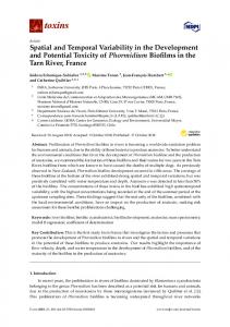
between data points over distance (Webster and Oliver, 2001). The location and result of each measurement is explicitly included in the analysis. Only recently have variograms been applied to shear strength and stability data (Kronholm, 2004) though variograms have been applied to other snowpack properties (Bloschl, 1999). A variogram is half the sample variance, the semivariance, plotted as a function of distance (Figure 2). The sill occurs where the semivariance “levels off,” typically corresponding to the overall variance of the dataset. The range is the distance to the sill, and is indicative of the spatial scale of the process (Bloschl, 1999). At distances beyond the range there is no longer correlation of results; measurement results are independent and not related. The nugget is the difference between zero and the semivariance at the shortest lag distance. The nugget is variance that cannot be resolved by the measured data (Myers, 1997). If there was no correlation in the data, the variogram would be a horizontal line, termed “pure nugget.”
Semivariance
Range
the pits within the plot, or the location of the test within the pit, does not matter. However, pit-to-plot ratios do provide a measure of the spatial variability within the data, and the representativeness of a pit for a plot. It provides practitioners with an indication of whether the results from one pit could be reliably extrapolated across the distance of a plot. 3. RESULTS AND DISCUSSION 3.1. Conditions prior to sampling A layer of near surface facets topped with surface hoar developed during a period of high pressure prior to January 22 2004. As early as January 10 the local avalanche center received reports of “nice surface hoar” (Chabot, 2004). Snowfall began on January 23, with approximately 25 cm of snow by January 24 (GNFAC, 2004). We sampled the alleys on January 26 2004 as the weather cleared and Plot 1 three days later. Sampling of the remaining plots occurred at near weekly intervals, with Plot 2 sampled on February 5, Plot 3 a week later on February 12, and Plot 4 sampled on February 20. Slab properties, weak layer strength and stability, and per day changes are summarized for the five sample days (Tables 1 and 2, and Figure 3). 3.2. The Alley, January 26
Sill
Nugget Distance Figure 2. Variogram, with parts important to interpretation labeled A “semi-spatial” method to characterize the spatial variability of a plot is the pit-to-plot ratio (Birkeland and Landry, 2002; Landry, 2002). Pit-toplot ratios characterize the ability of a single pit to represent the results of the entire plot. A pit is “representative” of the plot if there was no statistically significant difference between the results in a pit and the results of all the tests for a plot. The Wilcoxon Test was used to compare the individual pits to the pooled results. The Wilcoxon Test assumes only that the data distributions are symmetric. We pooled all results to increase the conservativeness of the test. If more pits represent the plot, the plot is less spatially variable. Pit-to-plot ratios are not spatial measures, because the locations of the tests are not explicitly considered in the analysis. The location of
No evidence from the alley samples suggested that any site-wide trends existed across the four plots. We found no significant linear trend in either the shear strength or stability data of the Alley sample. Therefore, we assumed similar initial conditions in all four plots. 3.3. Plot 1, January 29 Warm temperatures rapidly settled and consolidated the slab in the three days between the Alley and Plot 1 samples (Table 2). The surface hoar layer remained an avalanche hazard and a few avalanches were released in steeper, wind loaded terrain by the nearby Big Sky Mountain Resort ski patrol (GNFAC, 2004). At the study site it appeared that as the slab settled, the layer of facets above the surface hoar layer interpenetrated the surface hoar grains. The increases in both Plot 1 strength and stability were significant (p < 0.001) when compared to the Alleys. The QCV increased slightly, indicating an increase in the variability of shear strength. The shear frame test with the lowest shear strength was within 0.5 m of one of the tests with the highest shear strengths, suggesting spatial correlation only at short
distances. Such close proximity of very high and very low test results has been noted in other studies (Landry, 2002). On a per day basis, the change in median stability was an order of magnitude greater than observed between other sample dates (Table 2). This rapid increase occurred as the weak layer adjusted to the load of new snow. The increase in strength could have been accelerated as small facets penetrated the surface hoar layer, increasing the bonding and hence strength within the layer. 3.4. Plot 2, February 5 Light snowfall occurred throughout the week between sampling of Plots 1 and 2, increasing the median slab thickness to 47 cm. When we sampled Plot 2, grains in the oldest slab layers had begun to round. Again, small facets occurred between the surface hoar grains. The difference in strength between Plot 1 and 2 was significant (p < 0.001). The QCV of shear strength decreased when compared to Plot 1, indicating a slight decrease in the relative variability of the test results. The slight decrease in median stability between Plot 1 and 2 was not significant (p = 0.211). Although shear strength increased rapidly between Plot 1 and 2 (Table 2), the additional snowfall increased the load on the weak layer by a proportional amount, and little net change in stability resulted. 3.5. Plot 3, February 12 Snowfall occurred for several days following the sampling of Plot 2, with the heaviest snowfall occurring on February 8 and 9. Observers noted several natural avalanches in the vicinity of the study
site, and surrounding ski patrols released several avalanches, but the reports did not mention if the avalanches failed on the surface hoar layer we were sampling (GNFAC, 2004). Strengthening continued between Plots 2 and 3 at a decreased rate compared to rates measured earlier (Table 2). The QCV of strength increased between Plots 2 and 3, and was higher than the earlier samples, indicating increased variability of shear strength as the layer aged. Median stability continued to decrease between the plots as stress from the slab continued to increase (Table 2), but the field crew did not feel that the avalanche danger had increased. Other, easier but poorer quality failures occurred on interfaces above the surface hoar layer in stuffblock and rutschblock tests. The failures above the surface hoar layer indicated that, while the surface hoar layer was still a critical layer, it was no longer the most critical layer in the snowpack. 3.6. Plot 4, February 20 Snowfall resumed between sample days, with 15-20 cm of dense snow falling on February 18 (GNFAC, 2004). Strength continued to increase significantly between Plots 3 and 4 (p < 0.001). The rate of change in shear strength between Plots 3 and 4 continued to decrease (Table 2). The decrease in the rate of change is consistent with previous experience (Chalmers and Jamieson, 2003; Jamieson and Johnston, 1999; Jamieson and Schweizer, 2000; McClung and Schaerer, 1993; Tremper, 2001). The QCV continued to increase, suggesting that shear strength continued to become more variable.
Table 1. Summary of slab properties, shear strength, and stability ratios for the five days of sampling. ALLEY Median Slab Thickness (cm) QCV Median Slab Density (kg m-3) QCV Size of surface hoar grains (mm) Median Shear Strength (Pa) QCV Median Stability Ratio QCV
45 0.018 98 0.041 6-8 764 0.091 2.3 0.092
PLOT 1 34 0.002 129 0.034 4-6 1049 0.093 3.5 0.099
PLOT 2 47 0.011 157 0.015 6 1648 0.060 3.4 0.067
PLOT 3 66 0.023 148 0.024 6 2118 0.096 3.1 0.108
PLOT 4 72 0.014 183 0.011 4 2256 0.107 2.5 0.111
Table 2. Per-day change in median strength, stability, and slab properties. Alley and Plot 1 3 95 0.42 -3.50 10.07 < 0.001 < 0.001
Between Number of days Change in median shear strength (Pa day-1) Change in median stability (day-1) Change in median slab thickness (cm day-1) Change in mean slab density (kg cm-3 day-1) p value, change in strength p value, change in stability
Plots 1 and 2 7 86 -0.01 1.86 3.99 < 0.001 0.211
Plots 2 and 3 7 67 -0.05 2.71 -1.15 < 0.001 < 0.001
Plots 3 and 4 8 17 -0.07 0.75 4.36 < 0.001 < 0.001
Spanky's
3500
Shear Strength (Pa)
3000 2500 2000 1500 1000 500 0
0
5
10
0
5
10
15
20
25
15
20
25
5
Stability Ratio
4 3 2 1 0
Days
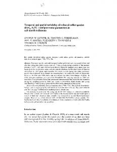
Figure 3. Box plots of shear strength (top) and stability ratios (bottom) through time. Dotted lines indicate plot medians, boxes indicate the 0.25 and 0.75 quantiles, whiskers the 0.05 and 0.95 quantiles, and circles the extreme values.
Median stability decreased significantly between Plots 3 and 4 (p < 0.001). The decrease in median stability of this layer did not seem to influence the avalanche hazard, and again the field crew felt that the surface hoar layer was no longer the most critical layer. The weaker interfaces above posed a greater avalanche problem. 3.7. Variogram Analysis Only shear strength was analyzed using variograms because of problems with stability calculations; we only measured one set of slab properties for each pit, which effectively reduced the variability of the stability results. In future studies, we hope to combine additional measures of slab properties with structural data from the SnowMicroPen. We found two significant linear trends within the stability data. Neither explained much of the variance, and we did not have enough measurements of slab properties to see if the slab had any spatial trends. Additional structural data, such as from the SnowMicroPen (Schneebeli et al., 1999), could be utilized to see if structural trends within the slab existed (Kronholm et al., in press), or if the linear trend was an artifact of the data collection and analysis. The four variograms (Figure 4) are “noisy,” with variations rather than increasing smoothly. None of the variograms indicated strong spatial correlation, and with the exception of Plot 1, all had very large nuggets. Several factors may cause large nuggets.
One cause could be that the correlation distance was short relative to the spacing of the measurements. The lack of data at shorter distances would mean that the correlation length is not well resolved. The additional, closely spaced tests from Plot 1 supported this possibility. Semivariance at the shortest distances, 0.4 m, on the Plot 1 variogram indicated a spatial pattern with correlation shorter than what could be resolved with the test array used on the other three plots. Additional support for correlation at short distances came from experience through the field season. If the operator felt a test was faulty, a second test was often placed as closely as possible to the first test. Unless the initial fault was due to an improperly prepared test, the second result tended to be more similar to the “faulty” test than two tests at the standard distance of 0.5 m. The test layout was designed to capture spatial correlation at distances of several meters. From this, it appears that there was significant variability and that there might have been correlation at distances less than 1 m over this slope. We hope to address correlation at short distances in future research. Large nuggets could also indicate noise in the measurements, or variability that the measurements cannot resolve (Bloschl, 1999; Myers, 1997). Our coefficients of variation ranged from 12 to 24%, which compared favorably with the coefficients of variation ranging from 3% to 66% (with a mean of 15%) reported by Jamieson and Johnston (2001) for 809 sets of shear frame measurements. This suggests that the large nuggets could be due to the test itself, and that there is considerable variation in shear strength that the shear frame test cannot resolve. 3.8. Temporal Changes in Spatial Variability
Figure 4. Variograms of shear strength for the four plots, from the top down, Plots 1, 2, 3, and 4. The horizontal scale, distance in meters, is common to all four variograms. The y axis, semivariance, differs between variograms as the semivariance increased through time.
There were no indications of site-wide trends in the Alley samples. We therefore assumed that the plots were initially similar, and attributed differences between the Plots to temporal change. Though we remain cautious about our spatial analysis given the quality of the variograms, there are a few points worth discussing. First, the nugget increased from Plot 1 to Plot 2 to Plot 3, indicating a larger amount of “noise” in the results and reflecting the lack of tests at close distances in Plot 2 and 3. There was little change in the nugget or range from Plot 3 to Plot 4, suggesting little increase in the noise. Second, in both Plots 2 and 4, the semivarince increased markedly between 2.5 m and 3.5 m. At those distances, tests were no longer within the same pit, so the increase indicated that there was more difference between pits than within pits.
3.9. Pit-to-Plot Ratios The only pits not representative of the plots were two pits of Plot 1. By the pit-to-plot measure, only Plot 1 demonstrated spatial variability. On all other plots, any individual pit statistically represented the shear strength or stability of the plot. By this measure, all other plots were spatially uniform. Of the four plots, the Plot 1 variogram indicated the least difference between tests at the inter-pits distances (all the variability occurred at distances within the pits), but Plot 1 had the only pits not representative of the plot. A pure nugget variogram or one that indicated spatial correlation at distances less than 2.5 m (the intra-pit distance) would be more consistent with the pit-to-plot results. We anticipated that more pits would not be representative of the plot based on Landry’s (2002; in press) study. In that work, over a third of the pits were not representative of the plots, while this research had only 2 of 16 pits (13%) that were statistically not representative. Several differences between the studies might explain the differences. One difference was the size of the plots. Our plots were about a fourth of the area of Landry’s, with distances between our pits about a fourth of the distance between Landry’s pits. Spatial trends at scales that Landry’s tests could pick up might be undetectable with our layouts. The type of test used was another difference between the current study and Landry’s work. Landry used the Quantified Loaded Column Test (Landry et al., 2001), which integrates slab characteristics into the test result. The shear frame test removes the slab from the test, and tests only the weak layer. This could account for some of the differences, if trends were present in the slab. 4. CONCLUSIONS AND IMPLICATIONS This study focused on three questions about spatial structure, temporal change, and causes of the change. Spatial patterns in the data proved elusive. Our variograms did not indicate strong spatial correlation. There may be several reasons; primary among them that the spatial correlation of shear results occurs at distances less than 1 m. Both Plot 1 and our field experience support such short correlation distances. In the coming winters, we plan to sample short distances more thoroughly. Another possibility is that we chose such uniform sites that we removed all spatial trends, leaving a nearly uniform slope that had no correlation or trends. If this were the case, the expected variograms would be pure nugget. Our variograms
were quite similar to pure nugget variograms, but they did exhibit some spatial structure. Our sampling array could be another reason we found little spatial correlation in the data. The array was designed to balance pit-to-plot ratios, geostatistical analysis, and the number of tests we could conduct on one day. Because geostatistical analysis proved more promising than pit-to-plot ratios at the scale of our study sites, arrays in the coming winters will better optimize the variograms, and ignore pit-to-plot ratios. Since our spatial analyses at this site did not show conclusive trends or spatial structure, we can make few conclusions about temporal changes in spatial variability. However, the significant changes in non-spatial measures of variability could be easily related to weak layer aging and changes in the slabinduced shear stress. Shear strength and the relative spread of the results increased through time as the weak layer aged and strengthened. This increase in spread across what our analyses show are relatively spatially uniform sites demonstrates how evaluating stability becomes more difficult and less reliable as the weak layer ages. We were able to follow the surface hoar layer from burial through strengthening to the point that it was no longer a critical weak layer for avalanching. Changes in stability were related to changes in the slab thickness, density, and weak layer aging. One issue that may be applicable to more than just this layer and slope is the correlation of adjacent tests. Commonly, stability tests are conducted adjacent to each other within a pit. If the correlation length of shear strength is, as indicated by this study, shorter that 1 m, results of these adjacent tests would be related, and under-represent the potential variability of stability or shear strength. To represent the potential variability adequately, tests would need to be spaced at distances greater than the correlation length, and a sufficient number of tests conducted to statistically represent the variability. The analysis allowed us to examine the ability of a forecaster to extrapolate stability tests. On this layer, over this uniform slope, stability results could be statistically extrapolated at least 17 m— provided sufficient tests were conducted to properly characterize the distribution of test results. How many tests are sufficient to characterize the plots? Sample size can be calculated many ways (there are easy to use sample size calculators at www.stat.uiowa.edu/~rlenth/Power/). A minimum of three uncorrelated tests would be necessary to insure, at a 95% confidence level, that the minimum stability ratio of the Alleys was not less than 1.5. By the time Plot 4 was sampled, ten tests would be
necessary. The margin of error is quite large with so few samples. To reduce the margin of error to within one standard deviation, 15 tests would be necessary under conditions similar to the Alley, and 18 under conditions similar to Plot 4. As the weak layer ages, more tests are required to adequately characterize the distribution of results. The test results must not be correlated, so, according to this study on this single slope, they should be spaced as much as a meter or more apart. Would this help to evaluate the avalanche hazard near the study area? Yes, but not directly. Because the surrounding, avalanche prone slopes are steeper and more wind affected than the study plot, results from the study area would need to be interpreted, just as most forecasting requires. 5. ACKNOWLEDGEMENTS Many thanks to Eric Lutz for all his help in the field in the summer and winter, for his assistance in organizing field days, and for his discussions on the ideas in this paper. We also thank Shannon Moore for his assistance in the field. Linda Bishop and Grant Estey facilitated site access. This research was financially supported by National Science Foundation (Grant #BCS-0240310). Spencer Logan was partially supported by the Barry C. Bishop Scholarship for Mountain Research and the Department of Earth Sciences at Montana State University. 6. REFERENCES Birkeland, K.W. and Landry, C.C., 2002. Changes in spatial patterns of snow stability through time, International Snow Science Workshop, Penticton, Canada. Bloschl, G., 1999. Scaling issues in snow hydrology. Hydrological Processes, 13(1415): 2149-2175. Chabot, D., 2004. Gallatin National Forest Avalanche Center Backcountry Observations. Chalmers, T.S. and Jamieson, J.B., 2003. A snowprofile-based forecasting model for skiertriggered avalanches on surface hoar layers in the Columbia Mountains of Canada. Cold Regions Science and Technology, 37(3): 373-383. Conway, H. and Abrahamson, J., 1984. Snow Stability Index. Journal of Glaciology, 30(106): 321-327. GNFAC, 2004. Gallatin National Forest Avalanche Center Backcountry Avalanche Advisories.
Gallatin National Forest Avalanche Center. Jamieson, B. and Johnston, C.D., 1999. Snowpack factors associated with strength changes of buried surface hoar layers. Cold Regions Science and Technology, 30(1-3): 19-34. Jamieson, B. and Johnston, C.D., 2001. Evaluation of the shear frame test for weak snowpack layers. Annals of Glaciology, 32: 59-69. Jamieson, J.B. and Schweizer, J., 2000. Texture and strength changes of buried surfacehoar layers with implications for dry snowslab avalanche release. Journal of Glaciology, 46(152): 151-160. Kronholm, K., 2004. Spatial Variability of Snow Mechanical Properties with regard to Avalanche Formation, Universitat Zurich, Zurich, 177 pp. Kronholm, K., Schneebeli, M. and Schweizer, J., in press. Spatial variability of penetration resistance in snow layers on a small slope. Annals of Glaciology, 38. Kronholm, K. and Schweizer, J., 2003. Snow stability variation on small slopes. Cold Regions Science and Technology, 37(3): 453-465. LaChapelle, E.R., 1980. The Fundamental Processes in Conventional Avalanche Forecasting. Journal of Glaciology, 26(94): 75-84. Landry, C.C., 2002. Spatial variations in snow stability on uniform slopes: Implications for extrapolation to surrounding terrain. MS Thesis, Montana State University, Bozeman, 248 pp. Landry, C.C. et al., in press. Variations in snow strength and stability on uniform slopes. Cold Regions Science and Technology. Landry, C.C., Borkowski, J.J. and Brown, R.L., 2001. Quantified loaded column stability test: mechanics, procedure, sample-size selection, and trials. Cold Regions Science and Technology, 33(2-3): 103121. McCammon, I., 2003. Using the shear frames, Snowpit Technologies, Salt Lake City. McClung, D.M., 2002. The elements of applied avalanche forecasting - Part I: The human issues. Natural Hazards, 26(2): 111-129. McClung, D.M. and Schaerer, P., 1993. The Avalanche Handbook. The Mountaineers, Seattle, 271 pp. Mock, C.J. and Birkeland, K.W., 2000. Snow avalanche climatology of the western
United States mountain ranges. Bulletin of the American Meteorological Society, 81(10): 2367-2392. Myers, J.C., 1997. Geostatistical Error Management: quantifying uncertainty for environmental sampling and mapping. Van Nostrand Reinhold, New York, 571 pp. Schneebeli, M., Pielmeier, C. and Johnson, J.B., 1999. Measuring snow microstructure and hardness using a high resolution penetrometer. Cold Regions Science and Technology, 30(1-3): 101-114. Spiegel, M.R. and Stephens, L.J., 1999. Schaum's outline of theory and problems of statistics. Schaum's outline series. McGraw-Hill, New York, 538 pp. Stewart, K. and Jamieson, B., 2002. Spatial variability of slab stability in avalanche start zones, 2002 International Snow Science Workshop, Penticton Canada. Tremper, B., 2001. Staying Alive in Avalanche Terrain. The Mountaineers, Seattle, 284 pp. Webster, R. and Oliver, M.A., 2001. Geostatistics for Environmental Scientists. Statistics in Practice. John Wiley and Sons, Chichester, 271 pp.