Temporal Coding Model of Spiking Output for Retinal ... - ThinkMind

COGNITIVE 2016 : The Eighth International Conference on Advanced Cognitive Technologies and Applications

Temporal Coding Model of Spiking Output for Retinal Ganglion Cells Philip Vance, Gautham P. Das, Dermot Kerr and Sonya A. Coleman School of Computing and Intelligent Systems, University of Ulster at Magee, Londonderry, N. Ireland. email: {p.vance, g.das, d.kerr, sa.coleman}@ulster.ac.uk Abstract—Traditionally, it has been assumed that the important information from a visual scene is encoded within the average firing rate of a retinal ganglion cell. Many modelling techniques thus focus solely on estimating a firing rate rather than a cells temporal response. It has been argued however that the latter is more important, as intricate details of the visual scene are stored within the temporal nature of the code. In this paper, we present a model that accurately describes the input/output response of a retinal ganglion cell in terms of its temporal coding. The approach borrows a concept of layout from popular implementations, such as the linearnonlinear Poisson method that produces an estimated spike rate prior to generating a spiking output. Using the wellknown Izhikevich neuron as the spike generator and various approaches for spike rate estimation, we show that the resulting overall system predicts a retinal ganglion cells response to novel stimuli in terms of bursting and periods of silence with reasonable accuracy. Keywords-Temporal coding; Spiking; Retinal Ganglion Cell; ANN; NARMAX.

I.

INTRODUCTION

Visual processing begins within the retina, which is a complex, networked organisation of cells comprising of photoreceptors, horizontal cells, bipolar cells, amacrine cells and retinal ganglion cells (RGCs). The retina contains approximately 1 million RGCs, each pooling a signal from multiple photoreceptors that define a spatial area known as a receptive field (RF). Light, upon entering the eye, is focused onto the photoreceptor layer effecting a change in each cell’s potential and forming a signal that is communicated through the various inter-processing layers to the RGCs. Here, the signal is changed into what are known as action potentials (spikes) and transmitted via synaptic connections to the visual cortex for higher processing. Modelling this input/output relationship has been a topic of interest over the years as studies have shown that strategies that utilise this biological aspect to visual processing outperform various machine vision techniques [1] in terms of power, speed and performance. The biological configuration of the retina makes it an ideal system for study as visual information (stimuli) can be controlled whilst physiological signals (response) can be recorded via a multi-electrode array from multiple RGCs before further processing begins [2]. The response for each cell is represented by a series of temporal spikes known as a

Copyright (c) IARIA, 2016.

ISBN: 978-1-61208-462-6

Thomas M. McGinnity School of Science and Technology Nottingham Trent University, Nottingham, United Kingdom. email: [email protected]

spike train, in which the processed information from the visual scene is considered to be encoded. Traditionally, it has been assumed that the important aspect of this coding is the rate at which the neuron fires on average [3] though others have argued that it is the temporal nature of the spikes, which carry the important information [4]. Evidence in support of the latter has been presented in various studies at multiple levels of the visual system [3]–[7] though depending on the stage of the visual processing, either one or a mixture of the two encoding representations may be relevant [2][5]. In [7], it is however reported that methods based on the mean firing rate in RGCs of a Poisson generated spike train, fail to account for the efficiency of information transfer between the retina and the brain. The emphasis is instead on the timing of the first spike across a population of RGCs to accurately describe the visual scene. In other work, brief bursts of spikes, post saccade (rapid eye movement), are thought likely to encode information pertaining to the encountered stimulus [2] and that the number of spikes within the burst are not necessarily as important as the time to the first spike. This would suggest that the importance in modelling the relationship between stimulus and response lies within matching bursts of spikes with particular emphasis on the first spike within the burst. Mathematical models of the relationship between stimulus and response in terms of the temporal code come in many variations with the simplest and most popular method stemming from a linear-nonlinear (LN) cascade approach using a Poisson process to generate a spiking output [8][9]. This method works on the premise that a spike rate estimation is generated first, followed by a temporal spiking output using a spike generating mechanism. Other variations propose the use of a leaky integrate and fire (I&F) neuron (or equivalent simplified model) at the latter stage of the model as it induces a more realistic comparison of the spike count variability, using a free firing rate, in cat and salamander RGCs, than that of the Poisson process, which is time-varying controlled [6]. In this work, extending from a previous comparison involving the I&F neuron [10], we propose to use the Izhikevich (IZK) neuron as the spike generating mechanism as it is more suited to reproducing spiking and bursting type behaviours [11], which can be finely tuned using a number of parameters. It differs from the I&F model in that the IZK model does not contain a constant firing threshold. This

83

COGNITIVE 2016 : The Eighth International Conference on Advanced Cognitive Technologies and Applications

infers a behaviour that is closer to real neurons; therefore the IZK model is better equipped, than the I&F model, to incorporate the critical regime of spike generation. Moreover, parameters in this model are tuned with a genetic algorithm ensures that the spiking behaviour of the IZK neuron is as close as possible to the RGCs behaviour. This is supported by an investigation into various methods for the estimated spike rate computation beginning with the standard LN cascade approach [12]. Results from the overall system show good performance in predicting the temporal code of a RGC, when presented with novel stimuli, in terms of bursts of spikes and periods of silence. In Section II, an overview of the experimental procedure used for the physiological experiments is provided along with data pre-processing techniques used to create an inputoutput dataset suitable for modelling. Methods used for spike rate estimation, spike generation, parameter tuning and temporal code analysis are presented in Section III with results for each phase presented in Section IV. Finally, Section V summarises the findings with a concluding statement. II.

dataset comprised of 1200 samples was presented to the same cell for testing purposes once initial characteristics had been formulated. This smaller dataset was presented repeatedly to the retina 43 times and could be used to observe the typical variance in neural responses from trial to trial. Both the physiological preparation and data collection were carried out at University Medical Center Gӧttingen, from which 36 RGCs were supplied with the identified size, shape and location of each RF. B. Data pre-processing As a pre-processing stage the stimulus values must first be extracted from each checkerboard pattern, illustrated in a stepwise procedure in Figure 2. To approximate the processing that occurs between the photoreceptors and RGCs, each checkerboard (Figure 2(a)) is fitted with a 2D Gaussian filter (Figure 2(b)), which accentuates the contrast levels within the visual scene [15]. Only pertinent values located either inside or on the border of the RF are extracted (Figure 2(c)) and summed to form an input dataset for modelling purposes.

EXPERIMENTAL OVERVIEW

A. Data Collection Physiological data were collected experimentally (in vitro) from adult axolotl tiger salamanders. Preparation involved isolating the dark-adapted retina, splitting into two halves and placing cell-side down onto a multi-electrode array, submersed in a chemical solution to prolong activity. Varying types of image stimulus inputs from a small OLED display were then focused onto the retina. Cell activations (via the multi-electrode array) were sampled at 10 KHz with spike times quantified with respect to the beginning of the stimulus presentation. Further details on the experimental setup and procedures can be found in [13][14].

Figure 2. Pre-processing step that shows how the local stimulus pertaining to a cell’s receptive field is weighted with a 2D Gaussian filter. (a) Local stimulus for a cells receptive field. (b) 2D Gaussian used to weight the stimulus intensities. (c) Weighted image of the local stimulus intensities.

The sampled neural response for each RGC is binned to match the frequency at which the stimulus is updated. For the non-repeated dataset, this formed the basis for model targets and output comparisons while for the smaller dataset the average of 43 trials was utilised as the output. III.

SPIKE GENERATION MODELLING

The aim of the work is to develop a biologically plausible spike generation model, i.e., one that will generate spikes at the same times as the actual RGC for the same stimulus.

Figure 1. Spatio-temporal checkerboard pattern.

In this work, artificial spatio-temporal stimuli (Figure 1) were used to determine the size, shape and location of each RGCs’ receptive-field through reverse correlation. The spatially arranged checkerboard patterns contain no spatial or temporal order and were presented to the retina at approximately 33 ms intervals. In total, the stimulus presentations numbered 258000 non-repeated samples to assemble a dataset large enough to ascertain characteristics, such as the Spike-Triggered Average (STA) and to ensure that a sufficient number of varied stimuli are presented in order to evoke cell responses. Furthermore, an additional

Copyright (c) IARIA, 2016.

ISBN: 978-1-61208-462-6

Figure 3. Overview of spike generation model.

84

COGNITIVE 2016 : The Eighth International Conference on Advanced Cognitive Technologies and Applications

In the widely used linear-nonlinear-Poisson (LNP) cascade model, spike generation is normally represented by a Poisson process [8][12][16], which is driven by the estimated spike rate. To this end, a cascade-type model (Figure 3) is developed to process the spatio-temporal stimulus and produce a spiking output in a two-stage process where initially an estimated spike rate is computed, which is then used to drive a spiking neuron. However, in this work instead of the Poisson process, a spiking neuron model is explored to further develop a biologically plausible spike generation model. Extending from previous work [25], we explore two well-known black-box methods and two transparent methods as a means for spike rate estimation. A. Spike Rate Modelling This section summarises the computational methods explored to model the estimated spike rate that drives the spike generation phase of the overall system. 1) Linear-Nonlinear: The linear-nonlinear (LN) model is one of the most popular methods for estimating a neuron’s spike rate as it is simple and efficient to implement [17]. It is computed by applying a linear filter to the input followed by a static nonlinear transform. Calculating the linear filter is typically achieved by computing STA, which is simply the average stimulus preceding each spike [12]. The main drawback is that the computed parameters of the model have no direct relationship to the underlying biophysics. 2) Artificial Neural Networks: Artificial Neural Networks (ANN) have been used extensively in the field of image processing, computer vision and similarly in the field of the biological vision system [15][18]. Designed as a network of artificial neurons to model task related properties of the cognitive process [19], they excel in pattern recognition and classification problems. An important goal of an ANN is to have good generalisation over its inputoutput mapping so that it can easily manage data that are slightly different to those upon which the network was trained [19]. One of the main drawbacks however is that, with too many training examples, the network may over fit the training data, meaning it can memorise specific traits of the training dataset, which are otherwise absent from further examples presented for testing resulting in poor performance. Bayesian Regularised Neural Networks (BRNNs), on the other hand, attempt to limit this inhibiting feature by restricting the magnitude of the weights to provide structural stabilisation [20][21]. Overly complex networks are thus reduced by effectively driving unnecessary weights to zero and calculating an effective number of parameters [21]. 3) Self-Organising Fuzzy Neural Network: Another way of reducing overfitting is to use less neurons within the network. This can further complicate matters by introducing the need to regulate the network size, as well as the number

Copyright (c) IARIA, 2016.

ISBN: 978-1-61208-462-6

of effective parameters unless the network is selforganising. In this work, we utilise the Self-Organising Fuzzy Neural Network (SOFNN) described in [22], which is a flexible, data driven model. This SOFNN was first introduced in [23], extended in [24], and is capable of selforganising its architecture by automatically adding and pruning neurons as required depending on the complexity of the dataset. This alleviates the requirement for predetermining the model structure and estimation of the model parameters as the SOFNN can accomplish this without any in-depth knowledge of neural networks or fuzzy systems. Bias 1

ᴨ1

N1

X1

X2

A1

A2 2

ᴨ2

N2 Au

Xr u

Input Layer

EBF Layer

ᴨu

Nu Normalised Layer

Weighted Output Layer Layer

Figure 4. SOFNN Architecture

The architecture of the SOFNN is comprised of five layers (Figure 4) that include an input layer, ellipsoidal basis function (EBF) layer, normalised layer, weighted layer and output layer. The EBF layer neurons do not need to be preconfigured as they are organised by the network automatically. In this layer, neurons are added or pruned during the learning process to achieve an economical network size. With each EBF neuron being a T-norm of Gaussian membership function (MF) attributed to the networks inputs, the if-part of the fuzzy rule is observed. Also, MFs found to share the same centre during the learning process can be combined into a single function, which allows the network to reduce the overall number of rules created. The consequent then-part, upon being normalised in the third layer, is processed by the weighted layer. The weighted layer is fed by two inputs: one from the previous layer and the other from a weighted bias. The product of these layers translates as the output to the final layer that contains a single neuron representing a summation of all incoming signals. Further detailed information on the SOFNN’s online learning capability can be reviewed in [23]–[25]. 4) Nonlinear Autoregressive Moving Average with Exogenous Inputs: Another popular method used when attempting to model the nonlinear relationship between input and output (stimulus and response) is the Nonlinear Autoregressive Moving Average with Exogenous Inputs (NARMAX) approach. The modelling is achieved by representing the problem as a set of nonlinear difference equations and is an expansion of past inputs, outputs and

85

COGNITIVE 2016 : The Eighth International Conference on Advanced Cognitive Technologies and Applications

noise. Since its conception in 1981, the NARMAX modelling approach has come to represent a philosophy for nonlinear system identification consisting of the following steps [26]: 1) Structure Detection: determine the terms within the model. 2) Parameter Estimation: tune the coefficients. 3) Model Validation: analyse model to avoid overfitting. 4) Prediction: output of the model at a future point in time. 5) Analysis: analyse model performance and determine the underlying dynamics of the system. Determining the structure of the model is critical and there exists a range of possibilities to approximate the function including polynomial, rational and various ANN implementations [27]. The polynomial models offer the most attractive implementation concerning visual systems modelling, as they allow for the underlying dynamical properties of the system to be revealed and analysed. Further details on the NARMAX approach and how it is implemented with respect to biological vision data can be found in [18][25] B. Spike Timing Model 1) Izhikevich Neuron: The Izhikevich (IZK) neuron model [11], which is both computationally efficient and variable in terms of response patterns, is used in this work as a method of spike generation. Variable response patterns can be initiated by configuring the parameters (𝑎, 𝑏, 𝑐 and 𝑑) of the IZK neuron, which can be set to obtain different types of neuronal responses, such as bursting, chattering or fast-spiking (Figure 5) that have been observed in real neurons [28].

Figure 5. Small sample of spiking behaviours capable with the IZK neuron

We envisage that such a range of behaviours will be useful for modelling RGCs and we find that a combination of Intrinsically Bursting and Regular Spiking behaviours performs best based on the visual inspection of the neuronal recordings from the electrophysiological experiments [29]. A full review of the biological behaviour of single neuron can be found in [3].

Copyright (c) IARIA, 2016.

ISBN: 978-1-61208-462-6

2) Parameter Tuning (Genetic Algorithm): A further improvement to the spike generation model was achieved through configuring the parameters of the model to best match the response patterns of the RGC. Given the range of possible combinations for each of the parameters in the IZK neuron, a genetic algorithm (GA) implemented from the DEAP toolbox [30] was utilised to search for the optimum parameters on the training data. As this method aims to tune a single IZK neuron as a one-time process, the GA is well suited as it is simple to implement and removes the need for manually tuning the parameters. To form the input of the GA, the real response was binned to form a spike rate and used to drive the IZK neuron. For one generation, the parameters for the neuron were drawn from a population size of 500 individuals using the tournament selection method, which involves running a tournament for several individuals and selecting the one with the best fitness for crossover or mutation. Each individual comprises the four parameters (a – d), which are randomly generated within the confines of each parameters limit as described by [11]. Finally, the evaluation of the neurons output is carried out using Dspike as the fitness function. Dspike [31] is a metric used as a numerical estimator of the similarity between the target (real) and estimated neural response. This algorithm essentially penalises a non-overlapping spike and/or penalises the necessity to insert a spike where if none exist in the estimated trace but does in the target response. Thus, Dspike is sensitive to the timing of the individual spikes and is calculated using a two-step process. The first step consists of inserting or deleting a spike to match the estimated spike train to the real spike train and involves a cost=1. The second step consists of moving a single spike and defines the sensitivity to spike timing. The cost associated with moving the spike is proportional to the time period by which the spike is moved. For example, if two spike trains A and B are identical except for a single spike that occurs at tA in A and tB in B, then c(A,B) = q|tA – tB| where c is the cost and q is a parameter specifying the cost per unit of time to move a spike. The Dspike can then be calculated as the total cost associated with the transformation path from A to B. If moving a spike by a time period has the same cost as deleting it completely, it can be seen that the value of q determines the relative sensitivity of the metric to spike count and spike timing. In the implementation, a value of 0.25 is selected for q corresponding to the size of time bins (four). IV.

RESULTS

A. Spike Rate Estimation We present results for two cells from the data collected; one OFF type and one ON type. Table1 and Table 2 outline the results for the OFF and ON type respectively, which were obtained for the spike rate estimation, which constitutes the

86

COGNITIVE 2016 : The Eighth International Conference on Advanced Cognitive Technologies and Applications

first stage of the overall model. Results from machine learning methods were validated using 5-fold cross validation, with parameters selected using a grid search approach. Model accuracy is presented in terms of the RMSE between the predicted and actual binned spike rate. As observed, the BRNN and LN perform similarly with the BRNN presenting better training results for the ON type cell and both training and testing for the OFF type cell. Although the NARMAX and SOFNN do not perform quite as well as these two methods, they do provide the capability of analysing the underlying system dynamics to gain a better understanding of what is actually happening. This is because one can interpret both the fuzzy rules of the SOFNN [25] and the estimated polynomial function of the NARMAX [18] method. An overall performance increase in RMSE for all methods is observable for the novel dataset. As the dataset is comprised of the average of 43 trials, this increase can be attributed to the removal of noise in terms of naturally occurring spontaneous spikes [28]. Further analysis on these results are shown in Table 3, as an example, where a statistical t-test has been performed between the various methods employed to show that the difference between the BRNN and LN methods, when compared to the SOFNN and NARMAX methods is significant for the OFF type cell. The test is based on the errors observed between estimated spike rate versus the actual spike rate. A small p-value in this case, below 0.05 indicates that the difference in performance is significant. As observed, the p-values from this statistical test when comparing the LN and BRNN methods are high, indicating that both methods are similar thus the null hypothesis, that the errors observed in both are similar, cannot be rejected. However, when comparing either the LN or BRNN methods with the SOFNN or NARMAX, the p-values are below 0.05 indicating that the null hypothesis can be rejected as the difference in performance is significant. B. Spike Count Estimation The purpose of the spike count estimation within this work is to evaluate the performance of the GA in tuning the parameters of the IZK neuron. Each model (for both ON and OFF type cells) had the parameters tuned using 100 generations of a population size of 500 using both crossover and mutation as forms of manipulation of the individuals. The resulting spike counts produced by both models are shown in Table 4.

TABLE 1. SPIKE RATE ESTIMATION RESULTS FOR OFF TYPE CELL

Model

LN BRNN SOFNN NARMAX

RMSE for OFF type cell Model Training/Testing on Non-repeated dataset Training Testing 0.35 0.35 0.34 0.35 0.36 0.37 0.35 0.36

Copyright (c) IARIA, 2016.

ISBN: 978-1-61208-462-6

Novel Dataset Testing 0.27 0.27 0.30 0.28

TABLE 2. SPIKE RATE ESTIMATION RESULTS FOR ON TYPE CELL

Model

LN BRNN SOFNN NARMAX

RMSE for ON type cell Model Training/Testing on Non-repeated dataset Training Testing 0.38 0.38 0.37 0.36 0.39 0.38 0.39 0.38

Novel Dataset Testing 0.24 0.23 0.27 0.25

TABLE 3. COMPUTED P-VALUES FOR THE NOVEL DATASET FOR THE OFF TYPE CELL (TABLE 1).

Model LN BRNN SOFNN NARMAX

LN -0.85 0.0057 0.00024

BRNN 0.85 -0.012 0.0079

SOFNN 0.0057 0.012 -0.70

NARMAX 0.00024 0.0079 0.70 --

TABLE 4. SPIKE COUNT OF EACH RATE ESTIMATION METHOD AS A MEASURE OF THE GA’S PERFORMANCE.

Model Actual Experimental (Average of 43 trials) LN BRNN SOFNN NARMAX

Spike Count OFF type cell 41.16 37 41 46 47

ON type cell 65.56 68 69 77 69

As illustrated in Table 4, the spike counts for both the ON and OFF type cells are similar to the average spike count of 43 trials pertaining to the real response for the LN and BRNN approaches. Resulting spike counts for the SOFNN and NARMAX approaches are not as accurate however; they provide better transparency in terms underlying model dynamics [25]. TABLE 5. DSPIKE PERFORMANCE MEASURE OF THE TEMPORAL OUTPUT FOR EACH RATE ESTIMATION MODEL.

Model LN BRNN SOFNN NARMAX

OFF type cell 42.23 45.17 51.33 49.45

ON type cell 63.38 62.14 67.73 66.03

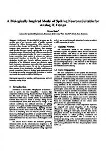
C. Temporal Coding The novel testing dataset, with the 43 repeated trials was used to test the spike generation performance. TABLE 55 outlines the main results in terms of the Dspike metric, which indicate that the IZK neurons driven by both the BRNN and LN methods are the top performers with the LN driven neuron performing better for the ON type cell and the BRNN driven neuron performing better for the OFF type cell. Figure 6 shows the predicted response plotted, for these two methods, in combination with a raster plot of all 43 individual trials for the OFF type cell.

87

COGNITIVE 2016 : The Eighth International Conference on Advanced Cognitive Technologies and Applications

used both the spike count and Dspike metric as a measure of performance. The resulting temporal code, again for the BRNN and LN methods, compared well against the real output though it is noticeable that the performance of the spike generation method is directly related to the performance of the machine learning approaches in predicting the spike rate, as they are cascaded. ACKNOWLEDGEMENTS The research leading to these results has received funding from the European Union Seventh Framework Programme (FP7-ICT-2011.9.11) under grant number [600954] (“VISUALISE”). The experimental data contributing to this study have been supplied by the “Sensory Processing in the Retina” research group at the Department of Ophthalmology, University of Gӧttingen as part of the VISUALISE project. REFERENCES

Figure 6. Raster plot of real neural response shown alongside the outputs of the LN and BRNN driven IZK neurons.

Visual analysis indicates the predicted spikes correlate well to the overall real neural response in terms of periods of nonactivity and periods of burst activity. Both methods perform almost identically except for the initial spikes that were missed by the LN approach and picked up by the BRNN approach. This negligible difference, which was absent within the spike rate estimation results, could be attributed to the Dspike configuration where the moving of a spike is only allowed if the spike, to be moved, resides within 4 time steps of its intended location, otherwise it must be deleted and reinserted. In terms of cost, this means that the deletion and reinsertion of a spike for the BRNN approach equates to 2 points whilst with the LN approach, there is only the need for a spike insertion. Also worth noting is that the IZK neurons driven by any method will retain repeatability in terms of producing the same spike trains each time. Since the IZK model is deterministic in nature, it lacks the ability to accurately reflect the random variability inherent in real biological systems, often observed as variations in spike times from trial to trial [3]. V. CONCLUSION AND FUTURE WORK In this paper, an investigation into the creation of a twostage temporal coding model has been presented where first a spike rate is estimated followed by a spike generation stage. The computational models reported for spike rate estimation were used to explore the development of a biologically plausible spike generation technique for spatio-temporal visual stimulus where the BRNN and LN methods were found to perform best though as the methods are opaque, further analysis of the underlying system dynamics is not possible. We evaluated the performance of the IZK neuron model cascaded with the spike rate estimation models and

Copyright (c) IARIA, 2016.

ISBN: 978-1-61208-462-6

[1] S. Shah and M. D. Levine, “Visual information processing in primate cone pathways. I. A model,” Sys., Man, and Cybern., vol. 26, no. 2, pp. 259–274, 1996. [2] T. Gollisch, “Throwing a glance at the neural code: rapid information transmission in the visual system.,” HFSP J, vol. 3, no. 1, pp. 36–46, 2009. [3] W. Gerstner and W. Kistler, Spiking neuron models: Single neurons, populations, plasticity. Cambridge Uni. press, 2002. [4] J. D. Victor and K. P. Purpura, “Nature and precision of temporal coding in visual cortex: a metric-space analysis,” J. of neurophysiology, vol. 76, no. 2, pp. 1310–1326, 1996. [5] J. Keat, P. Reinagel, R. C. Reid, and M. Meister, “Predicting every spike: a model for the responses of visual neurons,” Neuron, vol. 30, no. 3, pp. 803–817, 2001. [6] V. Uzzell and E. Chichilnisky, “Precision of spike trains in primate retinal ganglion cells,” J. of Neurophysiology, vol. 92, no. 2, pp. 780–789, 2004. [7] R. Van Rullen and S. J. Thorpe, “Rate coding versus temporal order coding: what the retinal ganglion cells tell the visual cortex.,” Neural Comput, vol. 13, no. 6, pp. 1255–83, 2001. [8] J. W. Pillow, L. Paninski, V. J. Uzzell, E. P. Simoncelli, and E. Chichilnisky, “Prediction and decoding of retinal ganglion cell responses with a probabilistic spiking model,” J. of Neuroscience, vol. 25, no. 47, pp. 11003–11013, 2005. [9] T. Gollisch, “Estimating receptive fields in the presence of spike-time jitter.,” Network, vol. 17, no. 2, pp. 103–29, 2006. [10] P. Vance, S. Coleman, D. Kerr, G. Das, and T. McGinnity, “Modelling of a retinal ganglion cell with simple spiking models,” IJCNN, 2015, pp. 1–8. [11] E. M. Izhikevich, “Simple model of spiking neurons,” IEEE Trans. Neural Netw., vol. 14, no. 6, pp. 1569–1572, 2003. [12] E. J. Chichilnisky, “A simple white noise analysis of neuronal light responses.,” Netw., vol. 12, no. 2, pp. 199–213, 2001. [13] J. Liu and T. Gollisch, “Spike-Triggered Covariance Analysis Reveals Phenomenological Diversity of Contrast Adaptation in the Retina,” PLoS Comput Biol, vol. 11, no. 7, 2015. [14] T. Gollisch and M. Meister, “Rapid neural coding in the retina with relative spike latencies,” Science (80-. )., vol. 319, no. 5866, pp. 1108–1111, 2008. [15] D. Kerr et al., “A biologically inspired spiking model of visual processing for image feature detection,” Neurocomputing, vol. 158, pp. 268–280, 2015.

88

COGNITIVE 2016 : The Eighth International Conference on Advanced Cognitive Technologies and Applications

[16] O. Schwartz et al. “Spike-triggered neural characterization,” J. Vision, vol. 6, no. 4, p. 13, 2006. [17] S. Ostojic and N. Brunel, “From spiking neuron models to linear-nonlinear models,” PLoS Comput. Biol, vol. 7, no. 1, 2011. [18] D. Kerr, M. McGinnity, and S. Coleman, “Modelling and Analysis of Retinal Ganglion Cells Through System Identification,” NCTA, 2014. [19] S. Haykin, “Neural Networks, A comprehensive Foundation Second Edition by Prentice-Hall,” 1999. [20] F. D. Foresee and M. T. Hagan, “Gauss-Newton approximation to Bayesian learning,” in Neural Netw., 1997., International Conference on, 1997, vol. 3, pp. 1930–1935. [21] D. J. Livingstone, Artificial Neural Networks: Methods and Applications. Humana Press, 2008. [22] E. Lughofer, Evolving fuzzy systems-methodologies, advanced concepts and applications, vol. 53. Springer, 2011. [23] G. Leng, G. Prasad, and T. McGinnity, “A new approach to generate a self-organizing fuzzy neural network model,” in Sys., Man and Cybern., 2002, vol. 4, p. 6–pp. [24] G. Leng, G. Prasad, and T. M. McGinnity, “An on-line algorithm for creating self-organizing fuzzy neural networks,” Neural Netw., vol. 17, no. 10, pp. 1477–1493, 2004. [25] S. McDonald et al. “Modelling retinal ganglion cells using selforganising fuzzy neural networks,” IJCNN, 2015, pp. 1–8. [26] S. A. Billings, Nonlinear system identification: NARMAX methods in the time, frequency, and spatio-temporal domains. John Wiley \& Sons, 2013. [27] S. A. Billings and D. Coca, “Identification of NARMAX and related models,” Research Report, Uni. Sheffield, 2001. [28] T. Trappenberg, Fundamentals of computational neuroscience. OUP Oxford, 2009. [29] S. Mittman et al. “Concomitant activation of two types of glutamate receptor mediates excitation of salamander retinal ganglion cells.,” J. of Physiology, vol. 428, p. 175, 1990. [30] F. Fortin et al. “DEAP: Evolutionary algorithms made easy,” J. Mach. Learn. Research, vol. 13, no. 1, pp. 2171–2175, 2012. [31] J. D. Victor and K. P. Purpura, “Metric-space analysis of spike trains: theory, algorithms and application,” Network: computation in neural systems, vol. 8, no. 2, pp. 127–164, 1997.

Copyright (c) IARIA, 2016.

ISBN: 978-1-61208-462-6

89