A temporal coding hardware implementation for spiking neural networks

A Temporal Coding Hardware Implementation for Spiking Neural Networks Marco Nuño-Maganda

Cesar Torres-Huitzil

Universidad Politécnica de Victoria (UPV) Av. Nuevas Tecnologías S/N Parque Científico y Tecnológico de Tamaulipas (TECNOTAM) Ciudad Victoria, Tamaulipas, México

Centro de Investigación y Estudios Avanzados (CINVESTAV-Tamaulipas) Parque Científico y Tecnológico de Tamaulipas (TECNOTAM) Ciudad Victoria, Tamaulipas, México

[email protected]

[email protected]

ABSTRACT

point), integer, boolean or string representation. But for SNNs, a dta representation in a spike train form is required. A set of input patterns must be mapped into a set of firing times, where the number of input neurons must be related to the number of input variables (or dataset columns). In case of string or boolean data (discrete values), one common technique consists on assigning integer values. When the input dataset is standardized for having only integer or real values, it is required to mapping these values to spikes or spike trains corresponding to firing times for each input neuron. This mapping operation could be considered generic, because both types of learning paradigms (supervised or unsupervised), will use the coding technique for passing the appropriate input values to the SNNs hardware module. One of the most used techniques for mapping real or integer values to spike times is the Gaussian Receptive Fields. This technique has a biological foundation, an it was used in [4] and [3] for both supervised and unsupervised learning. An argument against the GRFs is the high number of neurons used for mapping one dataset column (in the original paper, 12 input neurons are used, but several adaptation for using less neurons compared with the original trial have been reported). An argument in favor defined that GRF is a sparse coding scheme, which allows to distribute the input data range over a simplified (normalized) range. Inspired by the motivation of developing a high performance input data preprocessing module for several SNNs applications, we propose a parallel hardware architecture for GRFs that consists of a set of modular and flexible hardware modules. The motivation for implementing the GRF as an efficient hardware modules is that when processing complete datasets, it is desirable to parallelize several processing sequential tasks to speed up computations. As explained in the proposed architecture section, the GRFs coding can be obtained by a parallel hardware implementation, instead of a software implementation, allowing to other processing states to obtain a benefit related to the availability of the coding results, instead of obtaining the input coding in a sequential form. The originality of the proposed architecture consist on there are not hardware implementations related to temporal coding using GRFs for datasets reported in the literature. The proposed architecture can be de-

Spiking Neural Networks (SNNs) models have been explored in recent years due to its biological plausibility where temporal coding plays an important role. Biological arguments and computational experiments suggest than some perceptual tasks (vision and olfaction for instance) are well performed by these models. Moreover, some other applications such as machine learning might be benefited from this approach. However, efficient simulation and implementation of SNNs still remain an open challenge. There are several issues that must be addressed, being one of them the temporal coding of real-value data itself. In order to study the possibilities of embedded real-time implementations of large scale SNNs, we have first chosen to implement a well-known coding scheme based on Gaussian Receptive Fields (GRFs) to map real-value data into spike trains. This paper proposes a configurable parallel FPGA based accelerator for GRF-based temporal coding. The proposed architecture of the hardware implementation is described in detail and implementation results, both performance and resource utilization, when mapped to a Virtex-II Pro FPGA device are reported.

Categories and Subject Descriptors C.1 [Processor Architectures]: Parallel Architectures

1. INTRODUCTION Spiking Neural Networks (SNNs) have been widely used as an alternative paradigm for solving several applications, perception and Machine Learning (ML) to name a few, due to its temporal coding and generalization capabilities. In spite of their wide use, efficient simulations and implementations of SNNs still remain an open challenge since current computing engines are still far away from simulating large scale SNN systems efficiently. One of the most important issues to address for the implementation of SNNs is the temporal coding scheme and related algorithms to map real-value inputs to spike trains. Several techniques have been used, but each technique is strongly related to the addressed application (perception commonly uses a different coding than classification or clustering algorithms). For instance, in ML applications, the input datasets used for SNNs are stored using a real (fixed or floating

ACM SIGARCH Computer Architecture News

2

Vol. 38, No. 4, September 2010

fined as an specific purpose architecture, but with applications to a wide range of machine learning problems including both supervised and unsupervised learning for SNNs. The proposed architecture is important for accelerating interesting applications like image processing, speech processing, where the temporal coding can be applied with a potential possibility of success. SNNs and temporal coding using GRFs represent a new and different approach for solving traditional machine learning applications. The proposed paper is structured as follows. In section 2, the biological and mathematical background for GRFs are explained in detail. In section 3, the main modules of the proposed architecture are described. In section 4, the performance and hardware resource utilization results are explained. In section 5, a brief discussion of the potentials and limitations of the proposed architecture is presented. Finally, in section 6, conclusions and future work are provided.

From the point of view of the biological foundations of the population coding, input to the nervous system is in the form of five senses: pain, vision, taste, smell and hearing. Vision, taste, smell and hearing inputs are the special senses. Sensory input begins with sensors that react to stimuli in the form of energy that is transmitted into an action potential and sent to the Central Nervous System (CNS) [5] [13]. Sensory receptors are classified according to the type of energy they can detect and respond to. Neurons can be stimulated in various ways. There are specialized neurons that convert the physical energy of the environment into a neural signal. These neurons are called receptors. Visual receptors are found in the retina and they are responsible for converting light energy to an electrochemical neural signal for vision [10]. The receptive field of a sensory neuron is a region of space in which the presence of a stimulus will alter the firing of that neuron. Receptive fields have been identified for neurons of the following systems [6] [9]: the auditory system, the somatosensory system and the visual system. Characterizing the relationship between stimulus and response is difficult because neural responses are highly complex and variable. Neurons typically respond by producing complex spike sequences that react both the intrinsic dynamics of the neuron and the temporal characteristics of the stimulus. Isolating features of the response that encode changes in the stimulus can be difficult, especially if the same time scale changes in the same order as the average interval between spikes. Neural responses can vary from trial to trial even when the stimulus is presented repeatedly. There are many potential sources of this variability including variable levels of arousal and attention, randomness associated with various biophysical process that affect to neuron firing, and the effects of other cognitive processes taking place during a trial. Typically, many neurons respond to a given stimulus, and stimulus features are therefore encoded by the activities of large neural populations [11]. When trying to implement spike-based applications (i.e. image clustering or classifiers), a critical factor becomes the input encoding: as the coding interval is restricted to a fixed interval, the full range of the input can be encoded by using small temporal differences. Alternatively, the input could be distributed over multiple input neurons. The simulation of spiking neurons is iterated with a fixed time-step, an increased temporal resolution for the input values generates a computational penalty to the entire network [3]. This problem can be present when trying to use large datasets, and the range of the data contained in the dataset surpass the fixed interval assigned for the coding interval.

2. GRF-BASED TEMPORAL CODING The mammalian brain contains more than 1010 densely packed neurons that are connected to an intricate network. In every small volume of cortex, thousands of spikes are generated each millisecond [8]. Several issues about coding are of main interest: What is the information contained in such spatio-temporal patterns of pulses?, What is the code used by the neurons to transmit the information?, How might other neurons decode the signal? The previous questions have been addressed by the neurophysiology community and several mathematical models and approaches for information coding have been proposed: • Rate coding. The information is encoded in the neuron firing frequency. • Temporal coding. The information is encoded in the neuron firing time itself. • Population coding. The information is encoded by the activity of different pools (populations) of neurons, where a neuron may participate on several pools. There are strong debates about the question of which neural codes are used for biological neural systems, but there is a growing evidence that the brain may use all three coding approaches previously mentioned and combinations of them. The temporal coding seems to be specially relevant in the context of fast information processing [14]. There are several arguments in favor of population coding. The firing time, which could be defined as a temporal average over many spikes of a single neuron, only works well if the input is constant or if it changes on a time scale, which is slow with respect to the size of the temporal averaging window. Sensory input in a real-world scenario, however, is never constant. Moreover, reaction times are often short which indicate that neurons do not have the time for temporal averaging. Instead of an average over time, rate may be defined as an average over a population of neurons with identical properties [7].


2.1

Gaussian Receptive Fields

Datasets usually are collected from multiple resources and stored in the dataset repository. Resources may include multiple databases, data cubes or flat files. Different issues could arise during integration of data to be processed by SNNs. These issues include data transformation, which involves smoothing, generalization of the data, attribute construction, and input coding. In one dataset, each attribute has its own range. Data normal-

3


ization uses different techniques to narrow down values to a certain range. One of the most common normalization techniques is the min-max normalization. The min-max normalization performs a linear transformation on a set of data. Suppose that mina and maxa are the minimum and the maximum values for attribute A. Min-max normalization maps a value v of A to v’ in the range [nmina nmaxa ] by equation 1

GRF1

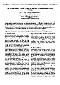
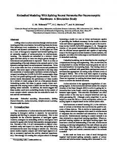
GRF1(0.3)=0.87126 GRF2(0.3)=0.97501 GRF3(0.3)=0.62169 GRF4(0.3)=0.22587

Using nmaxa = 1 and nmina = 0 to obtain a normalized dataset falling the the range [0,1], the equation 1 yields to:

1 m

0.5 0.4 0.3

0 −1

(2)

−0.5 0 0.5 1 1.5 Normalized Input Range (Coded Value:0.3)

2

Figure 1: Input value coding using 4 GRFs

GRF1

GRF2

GRF3

GRF4

GRF5

GRF6

1 Normalized Ouput Range (Firing times)

i − k1

0.6

0.1

(3)

Where the center b of the GF is given by equation 4 and the width σ of the GF is given by equation 5. bi =

0.7

0.2

For completing the coding task, one that the input data has been normalized, the normalized input data is used for obtaining the coding (each one represents an input spike that will be processed by the SNNs). One of the most common functions used for input data coding in SNNs is the Gaussian Function (GF), which is defined by equation 3. f (x) = ae

GRF4

0.8

v − mina ∗ (nmaxa − nmina ) + nmina (1) v = maxa − mina

(x−b)2 2σ 2

GRF3

0.9

0

v − mina v0 = maxa − mina

GRF2

1

(4)

0.9 0.8 0.7 0.6 0.5 0.4 0.3 0.2 0.1

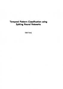
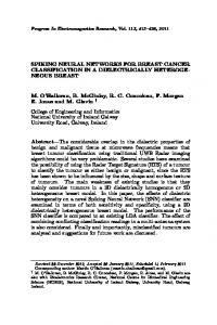
1 σi = (5) k2 ∗ m where k1 belongs to the range [0 − 1] and k2 belongs to the range [1 − 2]. There is not an exact value used for constants, only values obtained by trial and error are reported in previous applications that use GRFs for input coding. The GRFs consist on an array of GFs that are used for transforming a normalized input value I into a set of values evaluated by each one of the GFs that belongs to the array of GFs. This technique obtains a 1xM mapping for each input variable, where M is the number of GF used for mapping this input variable. This set of GFs have several applications reported in the past, like image clustering using SNNs [4] [2] [12] [1] and implementation of error-backprogating for multilayer SNNs [3]. The process of coding an analog value is shown in figures 1 and 2. In figure 1, an input value (0.3) is coded using 4 overlapped GRFs. In figure 2, the same value (0.5) is coded, but now using 6 overlapped GRFs. By the GRFs, it is possible to obtain the coding for any data independent on the input range, and it is possible to work with variables where several ranges are used.

0 −0.5

0 0.5 1 Normalized Input Range (Coded Value:0.5)

1.5

Figure 2: Input value coding using 6 GRFs

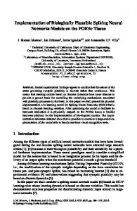
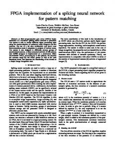
Figure 3: Main hardware modules of the proposed architecture

3. HARDWARE IMPLEMENTATION ACM SIGARCH Computer Architecture News

4


integer part, a LUT with the precomputed integer parts for each possible integer (numbered from 1 to 15) is used. For performing the computation of the fractional part, the series defined in equation 6 are computed in hardware, by the implementation of a set of multiply operations and the access to a LUT (BRAM memory) with the reciprocal of each factorial in the series. Finally, the results of both integer and fractional part are multiplied for obtaining the final exponential function. x3 x4 x2 + + + ... 2! 3! 4! Each GM contains the following modules: e(x) = 1 + x +

• Exponential Module (EM) - This module obtains the input data coding from the value located in the DP of the GM.

Figure 4: Main components of the EM

• BlockRam (BR) - This memory stores the firing times obtained by the EM.

In this section, the proposed modules for the hardware implementation is presented. In terms of the Flynn’s classification for parallel machines, the proposed architecture can be classified as a SIMD (Single Instruction Multiple Data), where several regular processing units process in parallel a set of input values for obtaining the input firing times. The main modules of the proposed hardware architecture are shown in figure 3. A detailed description of these modules is given below:

The main modules of each EM are shown in figure 3. The operation of the EM can be split into two parts: The left panel computes the min-max normalization required for each data to be codified (as defined by equation 2), and the right panel computes the exponential function given by 6, by dividing the computation process into two parts. The right panel computes the GRF using as input the normalization value obtained from the left panel. The main components of the GM are:

• External Memory Unit (EMU) - This memory contains the dataset to be coded. Several data lengths are supported, but for the proposed architecture, a 8 MBytes memory is used (organized as 1 MWords by 64-bits).

• Control Unit - Generated the synchronization signal required for each one of the components of the GM • Min Register (MR) - Contains the minimum value of the column dataset processed by the GM.

• Data Distribution Unit (DDU) - This unit defines how the input data are distributed to the processor modules.

• Bank of Centroids (BCs) - The number of registers of this bank depends on the total number of centroids (or input neurons) for each GRF. These centroids are computed based on equation 4.

• Gaussian Module (GM) - This unit performs the coding of one dataset variable using a set of GRFs.

• Integer Part Register (IPR) - The first part of the computation for each GRF is stored the IPR.

• Global Control Unit (GCU) - This unit defines when the GM performs the coding of the input time. This input data are performed in parallel, and the results can be stored in both external memory and internal memory for further improvements.

• Fractional Part Register (FPR) - The second part of the computation for each GRF is stored the FPR. • Bank of Reciprocals (BRs) - This memory contains the reciprocals of each factorial required for computing equation 6 (1/1!, 1/2!). The number of elements is fixed, and in this case, is set to 16.

Each GM has the following input ports: • Data Port (DP) - Contains the data to be processed. The width of this port depends on the number of columns to be processed in parallel.

• Reciprocal Register (RR) - Depending on the number of GRFs, the corresponding reciprocal is moved from the BR to the RR.

• Control Port (CP) - Contains several synchronization signals required for the operation of the GM.

• N-Power of FP Register (NPFPR) - The control unit defines how many times the FP register must be multiplied by itself for computing each one of the numerators of equation 6.

One of the main approaches for implementing the e function (required for computing each GRF) in hardware consists of using the form given by the series shown in equation 6. It is possible to divide the processing in two parts: the first one computes the result of the integer part, and the second one computes the result of the fractional part. For performing the computation of the


(6)

• Exponential of 1 Register (E1R) - This register is initialized to the fixed point representation for the evaluation of exp(1).

5


• Exponential Register (ER) - This register contains the final value of the computed GRF, and it obtained by multiplying the contents of both IPR and FPR.

Table 1: MSE achieved with several bit precisions bit precision MSE 8-bit 16.5 e-1 9.5 e-2 10-bit 6.17 e-2 12-bit 14-bit 7.23 e-3 16-bit 9.45 e-3

Several applications use a large number of GRFs, while others have proposed a small number of GRFs for temporal coding. The proposed architecture has been designed to be configured (in compilation time) for supporting a wide range of GRFs (as large as 16 GRFs, as defined in the original proposal, and as small as 4, as defined in a proposal defined in [15]).

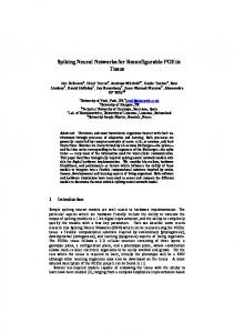
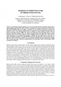
4. RESULTS The proposed architecture has been implemented on a Virtex-II PRO FPGA device. The target FPGA device is hosted on a Alphadata ADMXRC board, which hold a daughter PCM ADM-XPL board containing the target FPGA. The complete FPGA platform is hosted on a Pentium-4 PC (running at 2.66 GHz with 1 GB of RAM). The characteristics of the target FPGA devices is shown in table 2. Related to the performance of the proposed architecture, the implemented system is compared versus its equivalent software implementation, running on a Pentium-4 PC with 1 GB of RAM. The software implementation was coded using the Microsoft Visual C++ compiler, using the highest optimization settings available in the compiler. Regarding to the hardware implementations, each implementation was modeled using the Handel-C hardware description language and later it was validated on the target FPGA device. For showing the performance of the proposed hardware implementations, in figure 5 a comparison between both software and hardware implementations is shown. The legend “PC-4” represents the execution time of the SW implementation for a dataset with N samples (taken from the x axis) and 4 columns (variables). The legend “FPGA-4” represents the execution time of the proposed hardware architecture for a dataset with the same number N of samples and variables. The legend “PC-8” represents the execution time of the SW implementation for a dataset with N samples and 8 columns (variables). The legend “FPGA-4” represents the execution time of the proposed hardware architecture for a dataset with the same number N of samples and variables. In the SW implementation, all the processing is performed sequentially, while in HW, the implemented processors are used in parallel for performing the input coding. As it could be seen in the shown figure, the performance improves considerably (50x), but with the moderate the hardware resource utilization (around 30 percent of the FPGA device). Regarding to the data precision used in the proposed architecture, several variants of the proposed architecture were tested. For the current architecture, a 18 bit width register to store internal results and the resulting firing times was used. The change among precision variants was the number of bits used for fractional part (the remaining bits were used for the integer part). The Mean Square Error (MSE) is obtained for each one of the architectural variants. The hardware resources are the same for any variation of the proposed architecture, because only the precision is changed for each one of the


Figure 5: Performance comparison evaluated precision, but the register width is the same. In table 1, the obtained MSE for each tested precision is shown. In table 3, hardware resources and maximum clock frequency for each variation of the proposed architecture is shown. Each one of the reported implementations was validated on the target FPGA device.

5.

DISCUSSION

The base architecture is designed to be flexible for processing several GRFs with potential applications in different domains. For fast computing of GRFs, several EMs were used. The default configuration is 4 GRFs for each GM, but this configuration can be changed in configuration time. If the computation of 8 GRFs is required, then the same data is passed to two different GMs, and the obtained firing pattern is obtained by the concatenation of the output of the GMs assigned to the processing. The proposed architecture is designed to work with several columns of the source dataset. Even if the design of the DDU is modified, it is possible to have several sources for each column in the dataset, obtaining a potential performance improvement. The number of columns processed in parallel is given by the size of the EMU provided by the target platform and the available resources in the target FPGA. The importance of computing in parallel the temporal coding consists on the possibility of integrating the proposed architecture with any SNN in a pipelined fashion, when in one step of the computation the coding of the actual patterns is possible, and in the second step, the coding of the second pattern is performed meanwhile the processing of the spikes is performed in parallel.

6. 6

CONCLUSION AND FUTURE WORK Vol. 38, No. 4, September 2010

Table 2: Characteristics of the target FPGA device 4-Input Total Total Total FPGA LUTs Slice-FFs Slices BRAMs MULT18x18s xc2vp30-6ff896

27,392

27,392

13,696

136

136

Table 3: Hardware resources for the proposed hardware implementations Processors Slices Slice-FF 4-input LUTS BRAMs MULT18X18s Gate Maximum clock count frequency 4 1,515 1,583 2,153 1 25 408,807 85.7 MHz 11 % 6% 8% 1% 18 % 8 2,409 2,398 3,546 2 50 527,468 84.2 MHz 18 % 9% 13 % 1% 37 % 12 3,272 3,212 4,805 3 75 645,143 80.5 MHz 24 % 12 % 18 % 2% 55 % 16 4,018 4,031 6,054 4 100 762,048 76.5 MHz 29 % 15 % 22 % 3% 74 % At least 50X is obtained with the proposed architecture. Several performance-resource trade-offs can be established, since dedicated multiplier resources are the most demanded ones in the current implementation. If these resources are not available on the target FPGA, the proposed architecture should be synthesized to use only logic resources available on the target FPGA for implementing the multipliers required for the GRF processing. As future work, the integration of the proposed architecture with other processing modules for a complete implementation of SNNs will be analyzed (recall and learning for example). It is desirable to connect the proposed implementation into a fully integrated architecture, to show the functionality and interoperability for SNN processing, especially with image processing and pattern recognition.

[5] P. Dayan and L. F. Abbott. Theoretical Neuroscience. Computational and Mathematical Modeling of Neural systems. MIT Press, 2001. [6] M. Farabee. The on-line biology book. World Wide Web electronic publication, 1999. [7] W. Gerstner. Populations of spiking neurons. Maass, W. and Bishop, C., editors, MIT-Press, Cambridge, 1999. [8] W. Gerstner and W. Kistler. Spiking Neuron Models: Single Neurons, Populations, Plasticity. Cambridge University Press, New York, NY, USA, 2002. [9] E. M. Izhikevich. Which model to use for cortical spiking neurons? IEEE Transactions on Neural Networks, 15(5):1063–1070, 2004. [10] P. K. Kaiser. The joy of visual perception: A web book. World Wide Web electronic publication, 1996. [11] W. W. Lytton. From computer to brain : foundations of computational neuroscience. Springer, New York, 2002. [12] B. Meftah, A. Benyettou, O. Lezoray, and W. QingXiang. Image clustering with spiking neuron network. IEEE International Joint Conference on Neural Networks, pages 681–685, 2008. [13] M. Recce. Encoding information in neuronal activity. In Pulsed neural networks, pages 111–131. MIT Press, Cambridge, MA, USA, 1999. [14] B. Ruf. Computing and Learning with Spiking Neurons - Theory and Simulations. PhD Thesis, Institute of Theretical Computer Science, Technische Universitat Graz, Austria, 1998. [15] D. L. S. McKennoch and L. G. Bushnell. Fast modifications of the spikeprop algorithm. IEEE World Congress on Computational Intelligence (WCCI), July 2006.

Acknoledgments This work was partially supported by CONACyT-FOMIX Grant M0021-2009-23.

7. REFERENCES

[1] L. Bako. Real-time clustering of datasets with hardware embedded neuromorphic neural networks. High Performance Computational Systems Biology, International Workshop on, 0:13–22, 2009. [2] R. Berrêdo. A review of spiking neuron models and applications. Master’s thesis, University Federal de Minas Gerais, Brazil, 2005. [3] S. M. Bohte, J. A. L. Poutre, and J. N. Kok. Spikeprop: Error-backpropagation for in multi-layer networks of spiking neurons. Neurocomputing, 1-4(48):17–37, November 2002. [4] S. M. Bohte, J. A. L. Poutre, and J. N. Kok. Unsupervised classification in a layered network of spiking neurons. IEEE Trans. Neural Networks, 13(2):426–435, 2002.


7
