Temporal Difference Learning with Interpolated N-Tuples: Initial ...

Temporal Difference Learning with Interpolated N-Tuples: Initial Results from a Simulated Car Racing Environment Aisha A. Abdullahi, Simon M. Lucas

Abstract— Evolutionary algorithms have been used successfully in car racing game competitions, such as the ones based on TORCS. This is in contrast to temporal difference learning (TDL), which despite being a powerful learning algorithm, has not been used to any significant extent within these competitions. We believe that this is mainly due to the difficulty of choosing a good function approximator, the potential instability of the learning behavior (and hence the reliability of the results), and the lack of a forward model which restricts the choice of TDL algorithms. This paper reports our initial results on using a new type of function approximator designed to be used with TDL for problems with a large number of continuous-valued inputs, where function approximators such as multi-layer perceptrons can be unstable. The approach combines interpolated tables with n-tuple systems. In order to conduct the research in a flexible and efficient way we developed a new car-racing simulator that runs much more quickly than TORCS and gives us full access to the forward model of the system. We investigate different types of tracks and physics models, and also make comparisons with human drivers and some initial tests with evolutionary learning (EL). The results show that each approach leads to different driving styles, and either TDL or EL can learn best depending on the details of the environment. Significantly, TDL produced best results when learning state-action values (similar to Q-learning; no forward model needed). Regarding driving style, TDL consistently learned behaviours that avoid damage while EL tended to evolve fast but reckless drivers.

I. INTRODUCTION Car racing and driving is a rich environment with a variety of behaviours to observe and to test. Therefore, it has attracted a large number of researchers whether in real-world applications such as the DARPA challenge or in computer games such as the competitions held using TORCS (The Open Source Racing Car Simulator). Temporal Difference Learning (TDL), is a powerful, well-founded, natural, and incremental machine learning method that has proven its value in solving hard problems ranging from emulating helicopter maneuvers [1] to achieving expert levels of play in board games such as backgammon [2]. Despite that, TDL has not been a popular choice in the car racing context. We speculate that this could be due to a number of reasons: • Difficulty in choosing a good function approximator: this can be problematic when the problem involves a Aisha. A. Abdullahi and Simon. M. Lucas are with the School of Computer Science and Electronic Engineering, University of Essex, Colchester, United Kingdom, (email: {aamabd, sml}@essex.ac.uk).

978-1-4577-0011-8/11/$26.00 ©2011 IEEE

large number of continuous-valued inputs; Potentially unstable learning: this is especially true when using non-local non-linear function approximators such as Multi-Layer Perceptrons (MLPs); • More difficult to apply than evolution: because TDL can be sensitive to many choices such as learning rate, discount factor and the reward function; • Lack of a forward model: for some problems TDL works best when learning a state value function, but a forward model of the problem is required for this (i.e. to predict the next state of the agent and environment given the current state and the chosen action of the agent). Nonetheless, there is much evidence that TDL can learn extremely effectively when properly applied [3], [2]. Therefore, it is important to investigate how well it could work in the domain of car racing. The ultimate tests within this domain would involve driving real cars, such as in the DARPA. However, this involves a great deal of time, effort and expense. Simulated racing games can offer simpler and less expensive alternatives, and allow direct comparison of learning agents under identical conditions. In [4], a simple simulated car racing system was built, simplified to the extent that cars were just points in the track with basic dynamics and sensors, set to pursue randomly generated targets. Evolution and TDL were compared and also combined. TDL was found to be a quick learner, but highly unreliable especially with an MLP function approximator. Perhaps because of this, pure evolution was found to be reliable and have much better results overall. In [5], [6] more advanced simulators were built, with more realistic dynamics, traction and skidding effects, the presence of walls, and collisions being handled properly, though evolution was the central learning technique. Then the idea of organizing car-racing competitions emerged in CEC 2007 [7] where the competition was held based on an environment very similar to [4] but with more advanced dynamics. In that competition a representative number of techniques were applied, including one entry using TDL, a variety of evolved controllers such as those based on fuzzy systems, neural networks, and a few handcoded controllers. The evolved fuzzy controller was the winner of the competition though TDL was among the top 3 methods. •

321

The competitions have since been further developed to use TORCS, which is more engaging, realistic and 3D. The competition filters the controllers as follows. In the first warm-up stage it allows cars to recognize the environment, and then in the qualifying stage it eliminates the worst performing controllers. Later in the racing stage it races the qualifiers against each other. In [8], the results of the first competition in 2008 were described. In that competition there were no TDL controllers among any of the entries. The great majority of controllers tended to evolve a set of parameters selected by the developer. In addition to this, there was one hand coded controller that achieved third place. In 2009 the competition was extended to be a championship across three conferences, and has consequently attracted more competitors [9]. Two of the top five controllers were evolved fuzzy rule based systems, and the rest were utilizing evolutionary methods such as CMAES (Covariance Matrix Adaptation Evolution Strategy), and evolved neural networks. Moreover, all of these controllers were extensively hand-designed, usually at least partially hand-tuned. The rest were all hand crafted systems. The striking point is that TDL controllers were notable by their absence, and hence the performance of this important approach is largely unknown within this domain. Nonetheless, it is worth mentioning that in [10] a simple TDL method was implemented to learn only the overtaking behavior. In that system, all other tasks were adopted from an off-the-shelf controller. Their results show that TDL was able to outperform the strategy employed by one of the best drivers available in the TORCS distribution. The clear lesson so far is that designing TDL into a car racing system is something that has to be done with care, but when done well it can learn very effective behaviour.

computational intelligence for benchmarking purposes [9]. However, there are several difficulties that make it less than ideal for initial experiments with TDL controllers. Firstly, it is standalone software and the synchronization between the car controllers (driving agents) and the game itself is somewhat inconvenient. In addition, simulation time for TORCS is rather slow; According to [11], “simulation time for TORCS in batch mode is about 220 times real time, i.e. it takes 1 second to simulate 220 seconds of racing. Each second then contains 50 steps, which means that approximately 11,000 steps are simulated per second”. Finally, TORCS doesn’t provide convenient access to the forward model of the vehicle which prevents experimenting with TDL based on learning value functions. For these reasons we designed and implemented a new learning environment that replicates many of the aspects that are fundamental to the computational-intelligence competitions based on TORCS. Our simulator is much simpler than TORCS, but an agent sees a similar view i.e. it is endowed with a similar set of sensors to those used in the recent competitions such as [12]. In particular, it has the following features: • The capability of generating a large number of random tracks with minimal effort; • The model is fast to compute. This is important since machine learning techniques may require millions of simulated time steps in order to converge; • Highly configurable: different sensors, learning controllers, and alternative physics models can be plugged in; • Simple software interfaces. Finally, the simulator is implemented in Java, which was an important requirement to tie in with the code-base in our research group.

A. Paper overview This paper aims to introduce TDL to a simulated car racing environment and to further discuss major issues and limitations that TDL is usually faced with. First of all, to make the environment more flexible we developed our own simulator that presents a similar sensor model to the learner to the one used for the TORCS-based competitions, but is based on a simpler and more efficient physics model. Then, some theoretical background of TDL is provided, and our proposed function approximator is introduced to tackle the problem of unstable learning. A carefully selected implementation setup is explained afterwards, which is followed by several experiments addressing different learning challenges. The paper concludes with a discussion of the main results and proposed future work.

A. The Simulator The simulator uses computationally generated tracks, and simulates a car or several cars that can sense the environment and each other. Many other inputs are also available to the learning agent. The simulator runs significantly faster than TORCS and even faster than the simulator described in [11]. In our implementation, we were able to build a simulator that is 11,450 times faster than real time, meaning that given the same estimation for the single time step length it was simulating 114,500 time steps per second. In the following, all parts are briefly introduced and the software interfaces are provided. To see several snapshots of the simulator refer to track shapes in [13].

II. TORCS INSPIRED CAR RACING SIMULATOR TORCS is a widely used car racing simulator. It falls somewhere between being an advanced simulator, like the recent commercial games, and a fully customizable environment, like the ones typically used by researchers in

322

B. Tracks The idea of generating tracks has been implemented in several ways. In our implementation we build tracks based on basic geometry such as lines, ellipses and polygons. Then a mathematical function is plugged-in to give the track an entirely different shape. That function in our case is a summation of multiple sine functions which are controlled

2011 IEEE Conference on Computational Intelligence and Games (CIG’11)

by a variable x representing the car’s position on the track. Innovation is open when it comes to mathematical functions, and the interface to accommodate this in our software is as follows: public interface TerrainFunction { public double f(double x); } For full interaction with other parts of the environment, the track has to provide the following information: • Distance between two points, it is not as straightforward as it sounds. It is rather different according to the track basis geometry. For instance in the line track it is the progress in x position, whereas in the oval track it is the arc length between these two points; • The starting position and the angle which should be parallel with the track angle at that point; • Right and left points of the track at a certain point; • The distance from a specified point to left/right edge of the track; • The middle point of the track at any position.

III. REINFORCEMENT LEARNING A. General Ideology Interaction with the environment is the most basic and standard source of information for human beings to learn. Therefore, the replication of this process algorithmically is a key question and motive for machine learning researchers. Reinforcement learning is all about studying this interaction with the environment, consequences of actions, and maximizing rewards while achieving goals, [14]. The agent , where is the set of all possible starts from a state st states in the environment, then it selects an action at , where is the set of all possible actions available in the state st, and the environment responds to that action by giving a numerical reward, r , and moving the agent to a new state st+1, Fig. 1 sketches a car agent learning to drive. State of the world, st Reward, rt

Agent

Internal Model

Model copy(); Model copyAndUpdate(Action a); } The method reset is invoked place at beginning of each episode and it undertakes processes such as refueling, clearing the damage and so on. The update function is concerned with the real dynamics of the environment for example getting the next position of the car. The methods copy and copyAndUpdate are there to simulate “what if” conditions. The main parts of the simulator that are implementing the model are: the car dynamics with whatever physics model is used; details of the range sensors which are responsible for gathering information about the track; the opponent sensors providing knowledge about other cars on the track. Finally, the fuel, damage and the time related features are all set to implement it. As this is still a work in progress, more features could be added and due to this coherent model, all these parts are expected to interact normally with minimal changes.

Sensors

Actions at (forward/ backward) (left or right),

Fig. 1: A car agent learning in the environment.

public abstract class Model {

Model update(Action a);

Environment

Decision making

C. Models This part represents all the environment components that are interacting with the track. The main functionality of these models is encapsulated within the following interface whose methods enable the straightforward integration of TDL algorithms.

Model reset();

St+1

Theoretically, if this replication had the computational capacity, and was continuous and incremental, it could offer a strong solution to some serious real life problems. In the following, there are several flavors of this method, and a proposed function approximator that we believe offers an efficient and effective representation of the environment. B. Temporal difference learning and State/Action Value Functions TDL is one of the most popular methods in RL that stores all its experience in a value function. By following the temporal difference between the current and future states, the agent strives to maximize the reward signal and update the value function using the following formula: where V(st) is the value of a state s, α is the learning rate, and γ is the discount factor which is used to determine the present values of the future rewards. To use this method one needs a model of the environment, to project forward in time and get the value of these possible future states. When the forward model is not available one needs to learn an action value function (Q) rather than state value function (V), which has a very similar update:

2011 IEEE Conference on Computational Intelligence and Games (CIG’11)

323

,

, ,

,

This particular implementation of TDL is called SARSA, which is a shortcut to the whole process to be considered: the agent starts from a State, performs an Action, gets a Reward, enters the next State and selects another Action. It is also called on-policy learning method because the agent is updating its records according to its experience. Another variation is called off-policy learning, in which case the agent is not updating the value function from the experience but rather from a different policy. One of the best-known methods is called Q-learning which is greatly similar to SARSA, and uses this update formula: , , ,

,

where,

,

The only difference is that, Q-Learning updates its value function as if it has selected the best action while in reality it performs exploratory actions sometimes. These two methods had been widely used in the field, and which works best may be problem dependent. IV. FUNCTION APPROXIMATOR In tasks with small, finite states, it is possible to represent the value function using arrays or tables with one entry for each state (or state-action pair) [14]. This is called the tabular case, and the corresponding methods are called tabular methods. However when it comes to real world problems, the system state space is either very large or continuous which makes a direct tabular approach infeasible. The only way to learn anything at all is to generalize from previously experienced states to ones that have never been encountered before. That process is widely known as Function Approximation. There are two extremes to implementing tabular function approximators: the first is to roughly discretize the space which can lead to a very poor representation of the problem (i.e. significantly different states being dealt with in the same way). The intuitive alternative is to make a much finer discretization, in order to differentiate between all states. The downside of doing this is not just the large amount of memory needed but the time and data needed to access and train all possible system states. The exponential growth of table size with respect to the number of input dimensions is known as the curse of dimensionality. The goal of our proposed function approximator is to alleviate these issues by implementing interpolated table value function [15], for smooth function approximation, and then configure them as n-tuple networks to overcome the curse of dimensionality. In the following, a brief explanation for these terms is given along with the new proposed enhancement. A. Interpolated Tables The main idea behind interpolated tables is to use a weighted average value of the point neighbors. In a problem

324

of d dimensions and nq of possible discrete values, we map inputs to the range [0, nq], obtain the upper/lower bounds; the residual is the difference between the lower bound and the point. That residual is then used to determine how close the point is to any of its neighbors; hence the influence will be calculated. The interpolation is used to index the state while values are calculated during the learning process. The index computations are done as follows: ,….

1

, ,

, ,

0 1 0 1

This algorithm was previously applied to the mountain car problem using TD (0), and led to competitive results [15]. The main contribution of interpolated tables is that values can vary smoothly within each table cell. This provides a principled way to distinguish between the values of two states that are in close proximity, which in a naïve table would be tied to having identical values. It has been also proved theoretically to be stable and converging to the optimal functions [16]. B. N-Tuple Networks Traditionally n-tuple networks have used standard tables to store the learning value function [17]. The novel contribution of our function approximator is to use them with interpolated tables which make them far more suited to dealing with continuous inputs. Consider having a set of d input variables with m being the number of variables in each subset of d. The number of used subsets is obtained by ! !

!

which counts all possible combinations without

repetition. Using a simple combinations generator we can get all possible subsets of d. Now every subset will be treated as an interpolated table of with m inputs. The overall value for a state s will be the accumulated value of all different sub samples contained in s. The TDL update is done as follows: obtain the current value function from all the n-tuples, observe the next state and the reward value. Use the TDL error to update all the corresponding n-tuples indexed by the interpolation value of its variables. This function approximator has been applied before on a frequently used pole balancing problem [3] and proven attractive in terms of memory, training time, and smoothness of value function surface. It is able to form reasonable approximations to optimal value functions despite the sparse representation.

2011 IEEE Conference on Computational Intelligence and Games (CIG’11)

C. Hashing From our experiments with interpolated tables on simple problems, we observed that TDL usually finds a good solution without the need to visit the entire state space; indeed, for many problems much of the possible input space given the range of each input may well be infeasible. This sparseness can be further exploited in the design of interpolated n-tuple systems, by using hashing instead of arrays to store the values that occur. Indeed, depending on the configuration of the system, the array-based n-tuple systems may exceed the physical random access memory on a typical PC. To give a concrete example of hashing, this is how each hash map is declared within our Java code: Map vFunction = new HashMap ();

where State is wrapper class that is used to store the feature vector. To ensure the uniqueness of every state, the hash code was chosen to be as follows: i s x where d is number of dimensions and s is the number of discretization levels. Actually, this hash is the index of the state in a one dimensional table. Note that in CMAC related research, hashing was introduced to reduce the amount of needed memory [18], however, up to our knowledge hashing hasn’t been implemented before in combination with interpolated tables. In our implementation, it starts with an empty map, and then states and their values are added “as and when” needed. In the case of acquiring the value of a non-existent state, 0 or any other used initial value will be returned. The use of hashing tables here was a mere replacement for the table data structure, so the interpolation will be carried out as explained in IV.A which requires 2d visits to get the state. While training, it will start in a very fast manner as a result of the light memory usage. From several previously implemented problems we found that only 30%-70% of the state space was actually used, but for the problem at hand the table usage could be much sparser. V. EXPERIMENTS The objective of this work is to test the combination of TDL as the learning method and the proposed function approximator to represent the world in the car racing environment. This being the aim, the following experiments are designed to vary several aspects of the environment while keeping the algorithms constant, in order to verify results and examine the robustness of the learning process. Changes include track shapes, car dynamics, and starting states. We also performed experiments with evolving controllers, and several tests with human players. A. Experiments Setup To formulate the problem, we will first define state and action spaces, and rewards provided by the system. The state

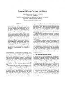
space of the race is factored to be represented by the following features: • 3 frontal range sensors (see Fig. 2); • The difference between the car and the track angles. • The car velocity; for the state value function the velocity components in x and y are provided. While in the action value functions the velocity magnitude is sufficient to represent the state.

Fig. 2: A view of the car and the ranges sensors are made visible for illustration.

Regarding the difference between state and action controllers with respect to the velocity feature, we found experimentally that providing velocity magnitude (speed) to the state controllers makes the state concept vague to the extent that even well trained controllers might drive backwards all the way to the end using a good trajectory. However, action controllers did not get affected by that, apparently coupling the state and the action in the value function makes it clear enough to learn good policies. In representing these features, the previously explained interpolated hashing n-tuples were used, with a tuple size of two, which produces 10 interpolated tuples based on the permutation rule explained in IV.B. Fifteen discretization levels were used. The action space constitutes the following actions: • Accelerate: (forward, neutral, backward); • Steer: (left, neutral, right); • Brake, (brake, no brake); the braking effect is integrated over time. All possible permutations of these actions are registered in an action list provided to the agent. Clearly, the ultimate goal in the race is for the car to finish the required number of laps in the minimum number of time steps while incurring no damage. However, applying a true reward based on this at the end of each episode to TDL controllers is hopeless because of the vast number of possible states and actions leading to the goal (or the end of the episode). In other words, with very distant rewards the temporal credit assignment problem can be too hard to solve. Therefore, we used shaping rewards which are practical and proven to be helpful if chosen carefully. Our reward, r , was the difference between the distance travelled and the deviation from the middle of the track. For the training process, every episode is made up of 500 steps for oval tracks and 1000 steps for line tracks. However, it would end before that if the controller was able to finish 10 laps, consumed the allocated amount of fuel, or exceeded the allowed damage limit. The notion of the lap in the line shaped tracks means 2000 distance units and for the oval

2011 IEEE Conference on Computational Intelligence and Games (CIG’11)

325

tracks means the entire circle i.e. 2π. For the oval track results, the lap 2π is multiplied by the radius, in our case 266.6, to get the arc length which is the distance the car has travelled, i.e. one lap is 266.67 * 2 * π = 1675.5 distance units. TABLE I TDL LEARNING PARAMETERS. Controller Exploration Learning rate ( ) rate ( ) Action 0.1 0.1 State 0.05 0.05

Discount factor ( ) 0.995 0.998

Finally, experimentally we found parameters in Table I to produce the best performing controllers for TDL under these conditions. To obtain reliable results for all experiments, they were averaged over 30 runs, unless otherwise stated. B. Easy Level We start by testing the learning process in several tracks where the driving process is supposed to be easier than others i.e. there are no sharp turns and the width of the track is fairly equal in all parts. For example if the track basic shape is oval, then there are no other curves added. The objective is to smoothly drive forward without bumping into track walls, since collisions with walls incur damage and cause the car to be pushed backwards. Results for the learning process are in TABLE II. In general, both state and action controllers have learned how to drive these tracks. From the figures in the table, the action controller was far better regarding distance, but somehow comparable when it comes to the rest of the statistics. Controller Action State Action State

TABLE II TDL TRAINING ON SIMPLE TRACKS Track Mean sDev Min Max Oval Oval Line Line

9581.33 1490.66 5701.34 11149.34 4797.33 1861.33 -1594.66 8176.01 10317.8 3319.4 5770.8 18177.07 4166.78 1149.73 2457.97 8278.74

Mean Damage 0.01 0.04 0.012 0.0

On the other hand from, detailed observations showed that the state controller did succeed from an early stage to follow a safe trajectory in the middle of the track but was very much slower than the action one. However, it is fair to say that the state controller was learning based on a bigger and clearer feature set. Learning in these cases usually proceeded slowly but steadily towards the optimal solution. Therefore, given a sufficient number of episodes, state controllers will eventually achieve similar results. To see driving clips refer to state and action controllers in [13]. C. Harder Level In this test a harder problem is posed, where the track shape gets highly unpredictable with narrow sharp turns if it is a line track, and with many curves added to the oval track. Results for state and action controllers on different tracks are in Table III.

326

Controller Action State Action State

TABLE III TDL TRAINING ON HARDER TRACKS Track Mean sDev Min Max Oval Oval Line Line

5546.67 4320.0 -2320.0 10660.68 4509.33 1338.66 0.0 7829.34 3462.8 2680.0 -861.6 10757.9 2669.15 118.8 2006.34 2794.70

Mean Damage 6.2 2.07 13.5 2.9

In fact some of these tracks were extremely hard to drive on, but the aim here was to test the performance limits of each controller. From the results, action controllers were usually able to drive reasonably well i.e. to finish several laps with acceptable damage record most of time. However, there were a number of bad runs among these and that explains the high standard deviation and the negative min value. Regarding state controllers, performance remained consistent with the previous results, driving rather slowly and with low damage recorded in comparison to the action controller. D. True Rewards vs. Shaping Rewards with State Controllers The above results show that action controllers have outperformed state ones. However, we hypothesized that this was due to the size of the feature set, which ensures quality solutions eventually but at a very slow pace. And we emphasize that our choice was important to give clearer representation for the states, and to obtain reasonable drivers. To investigate this further we designed a state controller that gets the true reward in a new way. Our aim was to see how well the state controllers can drive, and how much true rewards are different from the shaping ones we provided before. So, to implement that in a reasonable number of steps, we provided the shaping rewards in the action selection process as a heuristic. When the car finishes the entire episode it gets given the true reward at the end. Also, to make this possible the episode was reduced to only one lap during training, and back to normal, explained in V.A, while testing. The results for the line track are in Table IV. TABLE IV TRUE REWARDS FOR THE LINE TRACK (STATE CONTROLLER). Level Track Mean sDev Min Max Mean Damage Easy Line 14865.11 5895.8 -0.63 14865.11 0.47 Hard Line 6461.15 2613.22 568.21 11525.25 13.74

The improvement in the performance is enormous and shows how good state and all other controllers can be, if designed to absorb the true rewards or given full information and lifelong learning. However, providing the true reward in a learnable way is a hard problem and initial attempts to do this for the oval shaped tracks or for the action controllers were unsuccessful. E. Further Tests In the following, both controllers were presented with different challenging tasks such as driving using different dynamics. Also, their performance was compared with other intelligent drivers.

2011 IEEE Conference on Computational Intelligence and Games (CIG’11)

1) Different Dynamics In the above simulations, cars were modeled with simple motion dynamics involving no skidding or drag. In the following test, different dynamics that have skidding and traction effects are applied. This makes the cars much harder to control, and to partially accommodate that we use easier and wider tracks in these experiments. Results are listed in Table V. The highlighted rows for the oval tracks are to emphasize the poor performance: TDL did not learn to drive well under these conditions. Although both controllers have successfully driven in the line track, the action controller performance was roughly twice as good as the state one. In order to avoid skidding, both of them have converged to a very slow driving style. The state controller was better at minimizing the amount of damaged incurred. To observe an example of the car’s behavior refer to DynamicsAction in [13]. In the case of the oval track none of the controllers were able to complete a single lap, due to the constant attention to steering that oval tracks necessitate. Controller

TABLE V TDL TRAINING ON DIFFERENT DYNAMICS Track Mean sDev Min Max

Action State Action State

Oval Oval Line Line

528.00 392.00 4188.6 2853.42

472.00 18.66 1208.7 332.31

-482.66 349.33 1104.1 1817.78

1560.00 432.00 6659.2 5621.87

Mean Damage 5.94 0.0 9.47 0.05

2) Other Controllers In this part several tests were carried out to check the robustness of the learned controllers: • In the first test, a noisy starting state was used as a way to distract the learning process; results are in the second part of • Table VI. • In the second test, three human players were presented with a keyboard controller to drive around the track. They were allowed to get familiar with the track and control keys before recording their performance, to see the results refer to the third part of • Table VI. • The third test is detailed next in section 2.1. TABLE VI SEVERAL TESTS WITH TDL, RESULTS ARE AVERAGED OVER 10 RUNS. Controller

Start

Mean

sDev

Min

Max

Action State

Fixed Fixed

9847.9 13784.0

3199.9 642.80

3285.5 13001

15890.2 15140.0

Mean Damage 2.4 0.84

Action State

Rand. Rand.

7243.4 10561.8

3670.8 3495.43

-1166 0.0

15825.6 16231.6

5.1 0.15

1st player 2nd player 3rd player

Fixed Fixed Fixed

7086.5 7540.0 8709.5

514.4 866.1 673.3

6228.0 6035.0 7920.3

7629.9 8206.1 10090.8

15.3 14.6 9.4

All these tests were run on a mild difficulty line track and the results of normally configured controllers are in the first

two rows of the table. From these results the following observations can be made: • The first experiment, the true reward was used for the state controller and it clearly beats the action controller. However, both controllers were affected by the noise in the starting state (rows 3 and 4) to similar degrees. • The test with human players was by far the most exciting one to watch and to reason about. First point to notice is the very low standard deviation/high Min value which indicates a fairly reliable driving knowledge base. Typically, a human’s strong point was the far sightedness, whereas for the machine controllers this was limited to the length of the sensor. On the other hand, our controllers were better in quickly reacting to changes in the environment, and in driving optimally in the middle of the track most of the time. 2.1. Evolution and Random Search The results of third test against TDL were the most surprising. The test goal was to compare TDL with an evolved perceptron using a (15+15) Evolution Strategy (ES) evaluated on a neural state controller, the structure of the controller being similar to the one developed in [4]. The evolution was run for 100 generations and the fitness function was the difference between the normalized distance travelled and the damage endured. Evolution has exploited the simulator and learned a racing strategy that is to accelerate as much as possible without caring too much about minor damage. However, the best controllers have maxed out its performance in the allowed time slot with very low damage record. To see an average evolutionary controller in action, refer to the EvolutionaryController in [13]. Looking closely at the results we found that fitness was usually not being gradually evolved, but that good controllers could appear at random in any generation, sometimes even in the initial population. Hence to verify this, we also ran pure random search under the same conditions (i.e. same number of fitness evaluations). The unexpected finding was that pure random search did just as well as the ES. Furthermore, up to 10% of the randomly generated individuals were competitive with the best TDL drivers on this particular test, though often sustaining high damage. All of the successful perceptrons had the pattern of small random numbers with the following signs [-, -, +, -, -]. One specific example of such a perceptron weight-vector was: [-0.0061079, -3.92164707E-5, 0.001912191, -0.00854077, -0.0035025063].

Consequently, we think that the problem does have an inherent bias that makes it relatively easy to solve with a single-layer perceptron. Part of the reason is that recovery from a crash is rather easy, and many of these perceptrons use frequent collisions as part of their driving strategy. In the general RL literature there are occurrences of simple solutions that work efficiently comparing to more complex controllers, for example in [15] the author found an ultra-

2011 IEEE Conference on Computational Intelligence and Games (CIG’11)

327

simple rule that gives competitive results on the popular mountain car problem. We went further and tested whether this single-layer perceptrons could be evolved to control cars with harder dynamics, but no good perceptrons were found for the harder cases. Under the same difficult test conditions TDL was able to learn policies that were consistent with previous results, slow and cautious while the best evolved and randomly generated perceptrons seemed like a random driver. This indicates that good results from evolution and random search were exploiting particular features of that problem instance, whereas TDL was able to find good controllers under across a much wider range of problems. VI. CONCLUSIONS AND FUTURE WORK In this paper, temporal difference learning with interpolated hashed n-tuples was successfully used to train an agent to drive a simulated car. The simulator was inspired by TORCS but simplified to have superficially similar sets of tracks, dynamics, sensors, and features. Nevertheless, TORCS is superior to our simulator due to the fact it uses 3D representation of the dynamics, and the simulation of the drag, steering and damage are done in a more sophisticated way. Several experiments were conducted to test the smoothness and the robustness of the learned driving behaviours. In these tests, the action based controller was the best at finding the right balance between progressing along the track and maintaining a central track position. On the other hand, state controllers learned good driving behaviour from an early stage, but were rather slow and cautious in driving. We found that, although shaping rewards are easy to design, true rewards can enhance the performance if the system was carefully designed to allow access to the true reward. Our results are not directly applicable to TORCS controllers due to our simplified simulator. However, we have shown that at least in our simulator, a state-actionvalue controller which does not require a forward model is competitive with a state-value controller. This suggests that TDL may well be applicable to learning general driving behaviours in TORCS, and testing this hypothesis is important future work. Also to ensure quicker convergence, we are experimenting with high level actions, similar to those used in [10]. REFERENCES [1] P. Abbeel, A. Coates, M. Quigley, and A. Ng, "An Application of Reinforcement Learning to Aerobatic Helicopter Flight," in Advances in Neural Information Processing Systems, 2007, pp. 1-8. [2] G. Tesauro, "Temporal Difference Learning and TDGammon," Communications of the ACM, vol. 38, no. 3, pp. 58-68, 1995. [3] A. Abdullahi and S. Lucas, "Temporal Difference

328

Learning with Interpolated N-Tuple Networks: Initial Results on Pole Balancing," in for UK Computational Intelligence Conference, 2010, pp. 1-6. [4] S. Lucas and J. Togelius, "Point-to-Point Car Racing: an Initial Study of Evolution Versus Temporal Difference Learning," International Journal of Information Technology and Intelligence Computing, pp. 1-8, 2007. [5] J. Togelius and S. Lucas, "Arms races and car races," in Parallel Problem Solving from Nature (PPSN), 2006. [6] J. Togelius and S. Lucas, "Evolving Controllers for Simulated Car Racing," IEEE Congress on Evolutionary Computation, pp. 1906 - 1913, 2006. [7] J. Togelius et al., "The 2007 IEEE CEC simulated car racing competition," Genetic Programming and Evolvable Machines, vol. 9, pp. 295 - 329, 2008. [8] D. Loiacono, J. Togelius, P. Lanzi, L. Kinnaird, and S. Lucas, "The WCCI 2008 Simulated Car Racing Competition," in IEEE World Congress on Computational Intelligence, 2008, pp. 119 - 126. [9] D. Loiacono, P. Lanzi, J. Togelius, and E. Onieva, "The 2009 Simulated Car Racing Championship," IEEE Transactions on Computational Intelligence and AI in Games, vol. 2, pp. 131-147, 2010. [10] Daniele Loiacono, Alessandro Prete, Pier Luca Lanzi, and Luigi Cardamone, "Learning to Overtake in TORCS using Simple Reinforcement Learning," in IEEE Congress on Evolutionary Computation (CEC), 2010, pp. 1-8. [11] M. Jakobsen, "Learning to Race in a Simulated Environment," MSc. Thesis 2007. [12] The Open Racing Car Simulator. [Online]. http://torcs.sourceforge.net/ [13] Aisha Abdullahi. (2011) TDLRacing. [Online]. http://www.youtube.com/user/TDLRacing [14] R. Sutton and A. Barto, Reinforcement Learning: An Introduction.: The MIT Press, 1998. [15] S. Lucas, "Temporal Difference Learning with Interpolated Table Value Functions," IEEE Symposium on Computational Intelligence and Games, pp. 32-37, 2009. [16] S. Davies, "Multidimensional Triangulation and Interpolation for Reinforcement Learning," in Advances in Neural Information Processing Systems, 1996. [17] S. Lucas, "Learning to Play Othello with N-Tuple Systems," Australian Journal of Intelligent Information Processing, pp. 1-20, 2008. [18] Z. Wang, J. Schiano, and M. Ginsberg, "Hash-coding in CMAC neural networks," in IEEE International Conference on Neural Networks, vol. 3, 1996, pp. 1698 - 1703.

2011 IEEE Conference on Computational Intelligence and Games (CIG’11)