Temporal probabilistic modeling of bacterial ...

Bioinformatics doi.10.1093/bioinformatics/xxxxxx Advance Access Publication Date: Day Month Year Manuscript Category

Subject Section

Temporal probabilistic modeling of bacterial compositions derived from 16S rRNA sequencing Tarmo Äijö 1,∗ , Christian L. Müller 1 and Richard Bonneau 1,2,3,∗ 1

Center for Computational Biology, Simons Foundation, New York, USA, Department of Biology, Center for Genomics and Systems Biology, New York University, New York, USA, and 3 Courant Institute of Mathematical Sciences, New York University, New York, USA. 2

∗ To

whom correspondence should be addressed.

Associate Editor: Prof. Alfonso Valencia Received on XXXXX; revised on XXXXX; accepted on XXXXX

Abstract Motivation: The number of microbial and metagenomic studies has increased drastically due to advancements in next-generation sequencing-based measurement techniques. Statistical analysis and the validity of conclusions drawn from (time series) 16S rRNA and other metagenomic sequencing data is hampered by the presence of significant amount of noise and missing data (sampling zeros). Accounting uncertainty in microbiome data is often challenging due to the difficulty of obtaining biological replicates. Additionally, the compositional nature of current amplicon and metagenomic data differs from many other biological data types adding another challenge to the data analysis. Results: To address these challenges in human microbiome research, we introduce a novel probabilistic approach to explicitly model overdispersion and sampling zeros by considering the temporal correlation between nearby time points using Gaussian Processes. The proposed Temporal Gaussian Process Model for Compositional Data Analysis (TGP-CODA) shows superior modeling performance compared to commonly used Dirichlet-multinomial, multinomial, and non-parametric regression models on real and synthetic data. We demonstrate that the nonreplicative nature of human gut microbiota studies can be partially overcome by our method with proper experimental design of dense temporal sampling. We also show that different modeling approaches have a strong impact on ecological interpretation of the data, such as stationarity, persistence, and environmental noise models. Availability: A Stan implementation of the proposed method is available under MIT license at https://github.com/tare/GPMicrobiome. Contact: [email protected] or [email protected] Supplementary information: Supplementary data are available at Bioinformatics online.

1 Introduction Microbial ecology involves the study of microorganisms’ relationships with each other and with their environment and aims to provide insights into structure and dynamics of ecological networks (Kurtz et al., 2015), ecological stability (Faith et al., 2013), biodiversity (Lozupone et al., 2012), and discovery of key taxa in ecosystems (Ivanov et al., 2009). 16S ribosomal RNA (rRNA) amplicon sequencing (targeted nextgeneration sequencing of 16S rRNA gene) has proven to be a cost-effective,

culture-free, and highly multiplexed method to identify and compare bacterial compositions present within biological samples across a wide range of habitats, including natural environments (Meron et al., 2012; Hell et al., 2013) and different host organisms (Kuczynski et al., 2012; Yatsunenko et al., 2012). While the majority of amplicon sequencing studies has been cross-sectional in nature or based on few selected time points, it has been recognized that longitudinal studies with the aim of mapping the trajectories of microbiota over time are a prerequisite for a deeper understanding of ecological mechanisms in the microbiome and for the development of microbiome therapies (Gerber, 2014; Fisher

© The Author(s) 2017. Published by Oxford University Press. This is an Open Access article distributed under the terms of the Creative Commons Attribution Non-Commercial License (http://creativecommons.org/licenses/by-nc/4.0/), which permits non-commercial re-use, distribution, and reproduction in any medium, provided the original work is properly cited. For commercial re-use, please contact [email protected]

Downloaded from https://academic.oup.com/bioinformatics/article-abstract/doi/10.1093/bioinformatics/btx549/4157442/Temporal-probabilistic-modeling-of-bacterial by Simons Foundation user on 10 October 2017

Äijö et al.

2 and Mehta, 2014). Sparsely sampled microbial time series have already revealed dynamic reorganization of gut microbial compositions during early development in humans (Yatsunenko et al., 2012) and upon external perturbations through antibiotic treatment (Jernberg et al., 2010), and have identified significant differences in vaginal microbiota during pregnancy (Romero et al., 2014). The richest resource to date for long-term longitudinal amplicon studies are the landmark studies by Caporaso et al. (2011) and David et al. (2014) which provide human-associated microbial compositions on a daily time scale spanning hundreds of days. Caporaso et al. (2011) quantify natural variations of microbial compositions within and among four body sites across time. David et al. (2014) focus on the effects of host lifestyle, including travel, change of diet, and infection, on changes in the human gut microbiome. While statistical time series analysis has an extensive and successful history in classical genomics (Aach and Church, 2001; Bar-Joseph et al., 2004; Bonneau et al., 2006; Leek et al., 2006; Ahdesmäki et al., 2007; Bar-Joseph et al., 2012; Äijö et al., 2014), few attempts have been made to model amplicon-based temporal data in a principled statistical manner (Gerber et al., 2012; Bucci et al., 2016). This may stem in part from the fact that standard multivariate techniques can not be applied to ampliconbased sequencing data. Firstly, as compared to other technologies such as flow cytometry (Amann et al., 1990) and conventional plate counting that allow absolute taxa abundance measurements, standard 16S rRNA count data can only reveal relative abundances of taxa, thus rendering individual taxa counts not independent. Secondly, statistical analysis of 16S rRNA sequencing count data is complicated by the presence of overdispersion and missing data. Missing data manifests as an excessive number of zero counts due to imperfect sampling (i.e, zero-inflation and sampling zeros). Separation of sampling zeros (zeros due imperfect sampling) from structural zeros (true, biologically meaningful, zeros) is a common challenge in the analysis of many current biological data types, including single-cell RNA sequencing (Brennecke et al., 2013) and shotgun protein mass spectrometry data (Webb-Robertson et al., 2015). In the context of human-associated microbiome studies, ampliconbased sequencing studies face the additional restriction that well-controlled biological replicates (from different individuals) are not available due to different genetic background, environmental exposure, and life style of human subjects. Different approaches have been proposed to deal with these intrinsic characteristics of (cross-sectional) 16S rRNA sequencing data (see, e.g., Xu et al. (2015) for a recent comparison). Methods based on the negative binomial (NB) distribution (popular in modeling RNA sequencing data) have been proposed for modeling overdispersion in 16S rRNA data, and zero-inflated negative binomial (ZINB) and zero-inflated Gaussian (ZIG) (Joseph et al., 2013) mixture models have been successfully used to fit excessive numbers of zeros. However, the NB and ZINB distributions model taxa as independent, thus ignoring the intrinsic compositional nature of the data. Moreover, the binary distribution component of ZINB only increases the probability of zeros instead of modeling the source of zeros (true vs. non-detected due to sequencing depth) (Mohri and Roark, 2005). The impossibility of obtaining well-controlled biological replicates of human microbiome samples limits the applicability of NB distribution and ZINB in that context because overdispersion of (taxon-specific) counts caused by biological variation cannot be reliably estimated. In light of these limitations, several methodologies have been proposed for simultaneous modeling of taxa through their relative abundances, such as the Dirichlet-multinomial (DM) (Holmes et al., 2012; Chen and Li, 2013) and logistic normal multinomial models (Xia et al., 2013). The logistic normal multinomial model is a generalized linear model (GLM) utilizing the logit link function, thus enabling the use of wellestablished theory and methods of linear models for modeling count data

and relative abundances. Both models are extremely powerful for crosssectional studies with proper biological replicates. Yet, extending these models to time course data analysis has thus far been limited to pointwise analysis, followed by projecting the dynamics using low-dimensional embedding (Caporaso et al., 2011) or calculating different diversity metrics or temporal summary statistics across pairs of time points (Flores et al., 2014; Faust et al., 2015). Recent approaches that utilize the full potential of the data by considering temporal dependencies among the data points include MC-TIMME (Gerber et al., 2012) which uses exponential relaxation processes to model time-varying counts (Gerber et al., 2012) and BioMiCo (Shafiei et al., 2015) which uses a supervised hierarchical mixed-membership model to track groups of taxa over time. Other methods rely on deterministic regularized model fitting using generalized LotkaVolterra equations (Stein et al., 2013; Buffie et al., 2015; Bucci et al., 2016). In this study, we present a fully Bayesian probabilistic model, the Temporal Gaussian Process Model for Compositional Data Analysis (TGP-CODA), that tackles the compositionality, overdispersion, and zero-inflation in 16S rRNA sequencing data through temporal analysis. Our approach is based on the assumption that by sharing information across time points it is possible to improve inference of overdispersion and zero-inflation parameters. We demonstrate that our model can accurately distinguish sampling zeros from structural zeros by using the temporal correlation and the global effect of sampling zeros on the compositions. Our generative hierarchical model combines a multinomial distribution with Gaussian processes (for each taxon to model connections between time points), includes explicit model-based zero-inflation and overdispersion components, and can seamlessly integrate non-uniformly sampled time series (Section 2). We compare our temporal approach to the state-of-the-art DM model on realistic synthetic data and demonstrate more accurate composition estimation. We also model and reanalyze the long-term longitudinal gut microbiota data sets of four individuals (Caporaso et al., 2011; David et al., 2014) using TGP-CODA and maximum likelihood approaches (Section 3). We demonstrate (1) that the dynamical behavior of bacterial orders are globally stable but can accelerate upon environmental perturbations, (2) that our Bayesian model is robust to missing time points, and (3) that estimates of fundamental ecological indicators such as taxa persistence times and taxa stationarity are dependent on the underlying temporal model.

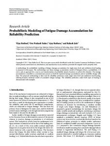
2 Methods We first describe TGP-CODA, our Bayesian generative model that integrates temporal, overdispersion, and zero-inflation components for analyzing longitudinal 16S rRNA sequencing data (Figure 1).

2.1 Data likelihood Let M be the number of taxa, T the number of measurement time points, (i) and T (|T | = T ) the set of measurement time points. Let xt be the number of observed reads assigned to the ith taxon at time point (i) t ∈ T (the corresponding random variable is denoted by Xi ), where every read is assigned exactly to one taxon. For notational simplicity, let (1) (2) (M ) (1) (2) (M ) xt = (xt , xt , . . . , xt )T and Xt = (Xt , Xt , . . . , Xt )T . Additionally, let us denote the total number of taxa assigned reads at time ! (i) point t by Nt = M i=1 xt . Next, let us assume: (1) Nt taxa reads are sampled independently of each other and (2) the M possible outcomes have fixed probabilities, Θt ∈ S M (M -dimensional simplex), at time point t. Then, Xt follows multinomial distribution with the parameters Θt and Nt Xt ∼ Multinomial(Θt , Nt ), t ∈ T .

Downloaded from https://academic.oup.com/bioinformatics/article-abstract/doi/10.1093/bioinformatics/btx549/4157442/Temporal-probabilistic-modeling-of-bacterial by Simons Foundation user on 10 October 2017

(1)

Temporal probabilistic modeling of bacterial compositions

Time evolution in real space

Sampling and biological variation in real space

θρ θσ

θη 2

η

ρ

2

σ

3 follows ! " ⎞ (1) exp Gt ! " # (i) M −1 ⎜ 1+ ⎟ ⎜ ⎟ i=1 exp Gt

⎛

2

⎜ ⎟ .. ⎜ ⎟ ⎜ ⎟ . ⎟, ! " Θt = Softmax(Gt ) = ⎜ ⎜ exp G(M −1) ⎟ ⎜ ⎟ t ! "⎟ ⎜ #M −1 ⎜ 1+ i=1 exp G(i) ⎟ t ⎝ ⎠ 1

G

T Compositions without noise ΘG M-1 and sampling T zeros Sampling zero θβ coefficients

F Compositions without sampling zeros

Θ

β

Θzi T M

x T

1+

The normal approximation to the multinomial (Severini, 2005), while computationally convenient, is not applicable in this case even for large values Nt because Θt is empirically observed to be located close to a corner of the simplex S M (i.e., there are many lowly abundant taxa). Next, let us define the likelihood in the case of multiple time points. Let us denote the collection of Θt over T time points by: (2)

The data likelihood assuming independence of observations at different time points (true for sequential sampling from a population) (Figure 1; see the “Likelihood” section), x = {xt |t ∈ T }, is "

t∈T

p(xt |Θt ) =

"

t∈T

#

Nt !

$M

(i)

i=1 xt !

M "

(i)

(i)xt

Θt

i=1

%

! " (i) exp Gt

(M )

Fig. 1. Statistical model and prior distributions. A graphical representation of our model. Grey and white circles depict observed variables and latent variables, respectively. Grey squares represent user-definable parameters. The Gaussian processes, G, model noise-free real-valued “compositions” (log odds ratios), which are used as a basis for generating noisy real-valued “compositions” (log odds ratios), F. Noisy compositions, Θ, are obtained from F by applying the softmax transformation. Zero-inflation-aware compositions, Θzi , are obtained from Θ and β by Θzi = Φ(Θ; β) (Equation (13)). The likelihood of data is evaluated using the zero-inflation-aware composition parameters, Θzi . Underlying unobservable noise-free compositions, ΘG , are obtained from G by applying the softmax transformation.

p(x|Θ) =

i=1

where Gt ∈ RM −1 (Bishop, 2006). The explicit assumption Gt =0 in Equation (4) makes the softmax transformation bijective. The softmax transformation is required because the multinomial likelihood parameters, Θt , are constrained to lie in the M -dimensional simplex. Next, let us denote the collection of Gt over T time points by

Compositions with sampling zeros Multinomial likelihood for taxa read counts

Θ = (Θt1 , Θt2 , . . . , ΘtT ) , where ti ∈ T , i = 1, 2, . . . , T.

#M −1

(4)

, (3)

which can be used to evaluate the likelihood of the data, xt , ti ∈ T given the parameter Θt .

2.2 Temporal modeling of microbiome compositions Modeling in compositional space is notoriously challenging (modeling fractions of population or fractions of reads, for example) (Aitchison, 1982): (1) the compositional space enforces restrictions on the modeling domain, which might not be easily expressible in the selected modeling framework (due to the intrinsic dependency among all taxa) and (2) the differences in relative abundances of taxa can vary over multiple orders of magnitude, which, combined with compositional effects renders the direct modeling of relative abundances a hard task. To overcome these challenges, modeling log odds ratios between taxa in real space have been proposed, typically followed by a transformation to map the real values to a simplex (Aitchison, 1982; Holmes et al., 2012). In this study, we will use the commonly used softmax transformation (e.g., in multinomial logistic regression) which is a generalization of the logistic function (Bishop, 2006). The softmax transformation from RM −1 to S M is defined as

G = (Gt1 , Gt2 , . . . , GtT ) , where ti ∈ T , i = 1, 2, . . . , T, (5) with the element-wise softmax transformation (see also Equation (2)) Θ = Softmax(G) = (Softmax(Gt1 ), . . . , Softmax(GtT )) . (6) Next, we will describe the temporal component of our generative model. It is unknown a priori how relative abundances of bacterial taxa vary over time and how treatments and abrupt changes in the environment might alter ecological dynamics. Therefore, we do not want to restrict the model and the resulting dynamics by strong assumptions on functional forms of temporal relative abundances. Thus, we will take a non-parametric approach and use a Gaussian process kernel to model temporal dynamics, requiring only weak assumptions (such as smoothness) on the temporal characteristics of the signal (Rasmussen and Williams, 2005). We assume that G(i) , i = 1, 2, . . . , M −1 (ith row of G) are smooth, and the time series data is well sampled (i.e., well-designed experiments to match the modeling objective). We will model G(i) , i = 1, 2, . . . , M −1 using Gaussian process (Rasmussen and Williams, 2005) T

G(i)

, ∼ GP 0, KG(i) (T , T ) ,

(7)

where KG(i) (T , T ) ∈ RT ×T , i = 1, 2, . . . , M − 1 is a symmetric and positive-definite covariance matrix ⎛ , , -⎞ k t1 , t1 |γG(i) . . . k t1 , tT |γG(i) ⎜ ⎟ . . .. ⎟ . (8) .. .. KG(i) (T , T ) = ⎜ . ⎝ ⎠ , , k tT , t1 |γG(i) . . . k tT , tT |γG(i)

, The term k ·, ·|γG(i) is the covariance function given the hyperparameters γG(i) . In this work, we use the squared exponential covariance function . / , ′ 2 k t, t′ |γG(i) = ηi2 exp −ρ−2 , i (t − t )

(9)

where γG(i) = (ηi2 , ρ2i ) with ηi denoting the signal variance parameter and ρi the characteristic length scale.

2.3 Modeling overdispersion of counts When the values Nt are large and no replicates are available, the data likelihood (Equation (3)) will dominate the Gaussian process prior (Equation (7)) leading to overfitting of Θt . Consequently, inherent biological and technical variations are severely underestimated. Notably, the DM and logistic normal multinomial models suffer from the same problem (this is apparent from the forms of maximum likelihood and Bayes

Downloaded from https://academic.oup.com/bioinformatics/article-abstract/doi/10.1093/bioinformatics/btx549/4157442/Temporal-probabilistic-modeling-of-bacterial by Simons Foundation user on 10 October 2017

Äijö et al.

4 estimators in SEquations (1) and (4), respectively). Thus, it is advantageous to explicitly model sampling variation in Θt , t ∈ T by introducing an additional level of random variables to the hierarchical model ⎛

⎞ F(1) ⎜ ⎟ .. ⎟, F=⎜ ⎝ ⎠ . (M −1) F

(10)

where F(i) ∈ RT , i = 1, 2, . . . , M − 1 are row vectors that depend on 2 as follows: G(i) and σ(i) F(i)

T

T

2 ∼ N (G(i) , σ(i) I) , i = 1, 2, . . . , M − 1,

(11)

2 is assumed to be constant over time (i.e., sampling variation is where σ(i) similar over time series) in order improve identifiability. In this extended model, Θ is obtained by applying the softmax transformation on F (see also Equation (2))

Θ = Softmax(F) = (Softmax(Ft1 ), . . . , Softmax(FtT )) , (12) where ti ∈ T , i = 1, 2, . . . , T . In summary, the random variable Θ = Softmax(F) (see Equations (11) and (12)) is sample-specific (after sampling), whereas the random variable ΘG = Softmax(G) (see Equations (7) and (6)) models biological variation over samples (before sampling). The overdispersion component of the model is illustrated in Figure 1 (see the “Sampling and biological variation” and “Observed compositions” sections).

2.4 Modeling zero-inflation and missing data 16S rRNA and other amplicon sequencing based count data have been empirically shown to suffer from severe zero-inflation (Xu et al., 2015). Zero-inflation can be seen as “salt” noise in the compositions Θt (i.e., zeroing of individual components of Θt ); the “salt” term refers to the “saltand-pepper” noise concept from the digital image processing literature (Jayaraman, 2009). To model zero-inflation, we introduce another level of simplex-valued latent variables, Θzi t , to the model (Figure 1). The variables Θt and Θzi model underlying proportions and “salty” proportions of taxa, t respectively. The sampling and zero-inflation are modeled separately for modeling convenience and for identifying the source of zeros (sampling or structural). To explicitly model the effect of imperfect sampling, we introduce (i) random variables βt ∈ [0, 1], i = 1, 2, . . . , M and consider the following weighting based transformation: ⎛

⎜ ⎜ ⎜ Θzi = Φ(Θ ; β ) = ⎜ t t t ⎜ ⎝

(1)

βt #M

(1)

Θt

(i) (i) i=1 βt Θt

. ..

(M ) (M ) βt Θt #M (i) (i) i=1 βt Θt

where the common denominator term ensures (i) {βt |t

!

⎞

⎟ ⎟ ⎟ ⎟, t ∈ T , ⎟ ⎠

(13)

Θzi t = 1. For notational

simplicity, let us denote β = ∈ T , i = 1, 2, . . . , M }. The zero-inflation component of the model is illustrated in Figure 1 (see the “Sampling zeros” and “Observed compositions” sections).

2.5 Posterior estimation To carry out the Bayesian inference on the presented model (Figure 1), 2 |θ ), p(ρ2 |θ ), we first specify the parameter prior distributions, p(η(i) η (i) ρ (i)

2 and ρ2 p(σ(i) |θσ ), and p(βt |θβ ) (SFigure 1a). The parameters η(i) (i) determine the signal variance and how fast correlation between time points

diminishes, respectively. We select a relatively broad prior distribution for ρ2(i) in order to support temporal correlations that vary from a few days to a few weeks (SFigure 1a). In this study, the time points ti (model inputs) are obtained by scaling the days of measurement (e.g., integers from 1 to D) by the total number of days (D); thus, the prior of ρ2(i) is selected as ρ2(i) ∼ N>0 (0.001, 0.005) (N>0 (·, ·) is positive truncated Gaussian distribution) (SFigure 1a). Since Gaussian processes model the log odds ratios, we assume that the variances of the log odds ratios of taxa over 2 ∼ Gamma(1.0, 0.5) time are relatively small. We set the prior as η(i) (SFigure 1b). The prior of the noise standard deviation is set to σ(i) ∼ N>0 (0, 0.5) to support relatively low noise levels (SFigure 1b). Finally, we explicitly assume that the sampling zeros, unexpected zeros from the multinomial sampling point of view, are relatively rare by defining the (i) prior as βt ∼ Beta(0.8, 0.4) (broad distribution improves sampling efficiency) (SFigure 1b). The posterior distribution function (up to a normalizing constant) is obtained as the product of the likelihood function and priors. The full posterior distribution function of our model is given in SEquation (5-6). We implemented the model in Stan (Carpenter et al., ress) and used its No-U-Turn Sampler (NUTS) to sample the posterior (SEquation (5)). The Stan probabilistic programming language enables cross-platform implementation, code interpretability, numerical stability, scaling, and efficient posterior inferences of various statistical models. Convergence of chains was monitored using by the Gelman-Rubin statistic (Gelman and ˆ < 1.1). All relevant information (prior and data) about Rubin, 1992) (R the parameters is summarized in the posterior distributions. We can thus use the obtained posterior samples to summarize the distributions, e.g., by calculating means and credible intervals (Gelman et al., 2014). It takes approximately an hour on a modern laptop to analyze a data set of 160 taxa and 27 time points.

3 Results 3.1 Temporal analysis improves estimation accuracy To validate the presented temporal compositional data analysis method, we first compare TGP-CODA to the DM model (Chen and Li, 2013) using synthetic data. To compare these two methods, we consider a scenario of 36 taxa with realistic dynamics and abundance distribution (see Supplementary Material). The generated synthetic data sets are analyzed using the temporal and DM models. The composition estimates at day 90 (common between six, nine, 14, and 27 time points to allow direct comparison) of both methods are compared to the noise-free ground truths (Figure 2a). Even in this simple scenario, the temporal approach consistently produces more accurate composition estimates than the DM model (Figure 2a; STable 1). We find that the performance of the temporal approach improves (as expected) as the number of time points increases; e.g., the mean estimation errors and the corresponding standard deviations are 0.15±0.09 and 0.10±0.06 with six and 14 time points, respectively (STable 1). The estimation error of the DM model does not depend on the number of time points as it considers time points separately (STable 1). To study the effect of sequencing depth on results, we repeated the experiment with lower sequencing depth (SFigure 4a). Also in the case of lower sequencing depth, TGP-CODA achieves better estimation accuracy than DM (SFigure 4a). Our modeling of temporal correlations and thereby sharing information between time points leads to more accurate estimation of compositions from longitudinal count data. Because our estimates should not be critically sensitive to the hyperparameters, (θη , θρ , θβ ). we carried out a sensitivity analysis with respect to the prior distributions of η 2 and ρ2 defined in the Section 2.5. We considered random variables θη,1 ∼ N>0 (1, 0.2) and θρ,1 ∼ N>0 (0.001, 0.00002) (SFigure 4b) whose purpose is to perturb the prior 2 ∼ Gamma(θ 2 distributions η(i) η,1 , 0.5) and ρ(i) ∼ N>0 (θρ,1 , 0.005).

Downloaded from https://academic.oup.com/bioinformatics/article-abstract/doi/10.1093/bioinformatics/btx549/4157442/Temporal-probabilistic-modeling-of-bacterial by Simons Foundation user on 10 October 2017

Temporal probabilistic modeling of bacterial compositions Number of time points 9 14

a Estimation error

6 p=0.06

p