1202
IEEE TRANSACTIONS ON NEURAL NETWORKS, VOL. 15, NO. 5, SEPTEMBER 2004
Temporally Sequenced Intelligent Block-Matching and Motion-Segmentation Using Locally Coupled Networks Xiaofu Zhang and Ali A. Minai, Member, IEEE
Abstract—Motion-based segmentation is a very important capability for computer vision and video analysis. It depends fundamentally on the system’s ability to estimate optic flow using temporally proximate image frames. This is often done using blockmatching. However, block-matching is sensitive to the presence of observational noise, which is inevitable in real images. Also, images often include regions of homogeneous intensity, where blockmatching is problematic. A better method in this case is to estimate motion at the region level. In the approach described in this paper, we have attempted to address the noise-sensitivity and texture-insufficiency problems using a two-pathway system. The pixel-level pathway is a multilayer pulse-coupled neural network (PCNN)like locally coupled network used to correct outliers in the blockmatching motion estimates and produce improved estimates in regions with sufficient texture. In contrast, the region-level pathway is used to estimate the motion for regions with little intensity variation. In this pathway, a PCNN network first partitions intensity images into homogeneous regions, and a motion vector is then determined for the whole region. The optic flows from both pathways are fused together based on the estimated intensity variation. The fused optic flow is then segmented by a one-layer PCNN network. Results on synthetic and real images are presented to demonstrate that the accuracy of segmentation is improved significantly by taking advantage of the complementary strengths and weaknesses of the two pathways. Index Terms—Block matching, image segmentation, locally coupled networks, motion estimation, motion-based segmentation, pulse-coupled neural network (PCNN), synchronization.
I. INTRODUCTION
L
OCALLY connected networks of synchronizable neural oscillators are interesting from both the neuro-engineering and computational neuroscience perspectives. Synchronization was proposed by Milner [27], Reitboeck [29], and von der Malsburg [33] as a possible mechanism for feature linking, experimental evidence for which was later reported [9], [10], [15], [16]. The use of synchronization as a neural information processing mechanism is especially interesting because it allows the use of fully spatiotemporal coding. Representations distributed over space (neurons) can be grouped or dissociated by changing the phase of their activities relative to each other, creating an extremely rich range of possibilities, and allowing time to be used for multiplexing several complex representations. This has led to the development of the pulse-coupled neural network (PCNN) Manuscript received July 2, 2003; revised December 4, 2003. This research was supported in part by a Grant from the Ohio Board of Regents. The authors are with Complex Adaptive Systems Laboratory, ECECS Department, University of Cincinnati, Cincinnati, OH 45221 USA (e-mail:
[email protected]). Digital Object Identifier 10.1109/TNN.2004.832817
model by Eckhorn et al.[10], and the locally excitatory, globally inhibitory oscillatory network (LEGION) model by Wang and Terman [35]. Both models have been applied to a variety of tasks in the areas of image analysis, auditory processing, and logical operation [6], [22], [23], [25], [28], [34], [36]. A major application for synchronizable networks is image segmentation: The partitioning of an image into objects or regions based on common characteristics [13], [14]. Approaches based on the PCNN and LEGION models have been quite successful in solving this problem, focusing mainly on intensity-based segmentation [10], [25], [31], [36], though LEGION has been applied to motion-based segmentation as well [7]. In a synchronization-based image segmentation scheme, each object is represented by a group of synchronized neurons, while different objects are represented by mutually desynchronized neuron groups. Methods based on synchronizable neurons are of special interest for two reasons. First, because of its neural paradigm, this approach is inherently amenable to parallel implementation. Second, it may help elucidate possible mechanisms in the early visual system and, thus, lead to more powerful computer vision methods. Motion-based segmentation, which refers to the process of partitioning an image into objects (regions) with common motion, is a fundamental problem in the fields of video processing, target recognition and computer vision. Quite often, objects in real images do not have homogeneous intensity, texture, etc., and are identifiable only by their coherent motion. Motion-based segmentation is closely related to the motion estimation problem. If a good estimate of the optic flow is available for an image, it can be segmented readily [20]. The simplest way to estimate the motion of a region is by block matching across image frames separated by short time intervals. However, block matching is often complicated by noise in the image, which creates spurious matches and, therefore, incorrect estimates of optic flow. This is particularly problematic in regions with little inherent texture, since most of the variation in that case is noise. The problem can be alleviated partially by spatial smoothing of the optical flow field [3], [32]. However, optic flow smoothing can blur the flow image at object boundaries, which is counterproductive for motion segmentation methods. Block matching also has difficulty with regions of homogeneous texture, and algorithms that combine motion segmentation and intensity segmentation have been proposed to deal with this [7], [8]. In these methods, intensity segmentation is performed first, followed by a unique motion estimate for each segment. In this paper, our objective is to present a method for translational motion segmentation using block-matching in combi-
1045-9227/04$20.00 © 2004 IEEE
ZHANG AND MINAI: TEMPORALLY SEQUENCED INTELLIGENT BLOCK-MATCHING
Fig. 1.
1203
Flow diagram of the system.
nation with PCNNs to alleviate the problems of image noise and texture insufficiency and provide reliable segmentation. We address the noise-sensitivity problem by spatially smoothing the optic flow through the local connections between neighboring neurons in a multilayer locally coupled network. A block-matching certainty measure is also defined to propagate the smoothing from reliably estimated motion vectors to the less reliable ones in the neighborhood. To tackle the texture insufficiency problem in homogeneous regions, a PCNN network first partitions intensity images into homogeneous regions, and a motion vector with maximum accumulated certainty is then assigned for the whole region. A key property of the system we present is that it uses networks of locally connected neurons that function through spreading activation and temporal multiplexing. The system is inspired directly by the LEGION approach of Çesmeli and Wang [7], which consists of two parallel pathways that process motion and brightness, respectively. Their system uses continuous-valued continuous-time synchronizable neural oscillators while we use discrete-time binary neurons (as in many PCNN models). The two models also differ in the specifics, but share the general approach of refining motion estimates based on block-matching, using complementary pathways, and separating segments by means of temporal coding. In a sense, the system we present can be seen as a simplified version of the approach in [6] and [7], and was developed in collaboration with the authors of that work. It is interesting to see how well even this simplified model
works, demonstrating the general utility of the approach. As far as practical, we have attempted to accomplish all tasks through spatiotemporally localized processes, which is one of the primary points of interest in this work. II. PROBLEM DESCRIPTION Given an image sequence , we consider two distinct temporally proximate frames and , . Using the two frames, the task for the system is to: 1) assign an optic flow vector to every pixel in ; 2) group together pixels that have sufficiently similar optic flow estimates and form a connected region. Each group is called a segment. Thus, the outcome of the processing is a labeling of each pixel by a segment identifier, presumably corresponding to a single object with rigid translational motion. III. SYSTEM DESCRIPTION The approach we present is termed temporally sequenced intelligent block-matching and motion-segmentation (TIBM), and is shown schematically in Fig. 1. The TIBM system comprises three stages. Stage I: Block Matching and Certainty Determination: In this stage, local block matching is applied to the image frames
1204
IEEE TRANSACTIONS ON NEURAL NETWORKS, VOL. 15, NO. 5, SEPTEMBER 2004
and , to obtain the best block-matching motion estimate (BBME), , for each pixel. In addition, a block, is also computed matching certainty measure (BCM), for each pixel. Typically, highly textured regions generate higher certainty values. These two quantities are then used as inputs for the next stage. To facilitate processing, we normalize intensities in all images to the 0–1 range. Stage II: Refined Optic Flow Estimation: This is the main processing stage where the estimates from Stage I are refined using the BCM values and neighborhood information. Stage II processing comprises two pathways: the pixel-level (P) pathway and the region-level (R) pathway. The basic idea is to partition the image into two types of regions: Textured regions, where detailed block matching can work well and noise is the main problem, and homogeneous regions, where block matching is inherently uncertain because the information (texture) needed for it is lacking. The P pathway uses a multilayer locally coupled network to identify the textured regions and performs adaptive local smoothing to produce high-quality optic flow estimates for these regions, while the R pathway uses a standard PCNN to detect homogeneous regions and heuristically assigns uniform optic flows to them based on the BBME of the regions with maximum accumulated certainty, which usually correspond to local features or neighboring textured regions. Thus, the regions best suited to block matching end up with reliable flow estimates, while regions not suited to block matching in the first place are isolated and handled separately. As such, our approach can be seen as a type of “intelligent” block matching. Stage II processing produces two optic flow images from the P pathway, and from the R pathway, and a , which indicates which estimate should be used mask for each pixel. The optic flow images are then combined through the mask to produce the final optic flow image (1) Stage III: Segmentation: In this stage the optic flow image, , produced by Stage II is segmented using a standard onelayer PCNN, following the approach used for intensity-based segmentation in [21], [25], [36]. We now describe each stage in detail.
The best block-matching motion estimate (BBME) for pixel is if for all in the search neighborhood. We use to denote the BBME for pixel . The SAD values for over all displacements can be seen as forming a surface, , whose curvature provides information about the certainty of the match. Intuitively, the best match on a flat SAD surface indicates a random choice in a low textured region, whereas a best match in a deep trough corresponds to a higher certainty estimate [4], [6]. Using this idea, we define a simple, efficiently computed certainty measure for block matching. The block-matching certainty measure for the best match displacement, (BCM) at pixel is defined as
(3) denotes the eight immediate neighbors of the diswhere placement on the surface. The denominator includes a small constant to prevent division by zero. All s are then normalized by the maximum in the whole image so that . In [4], distinct certainty measures are defined along two components of the motion vector, while in [6], certainty is calculated along the direction perpendicular to the motion vector. The directional definition of certainty is very useful in many cases, e.g., in solving the aperture problem. However, the major objective of our method is to eliminate the outliers caused by noise. Thus, we need a nondirectional certainty measure to spread the smoothing activity to all neurons in the neighborhood. Although our certainty measure is considerably simpler, it is interesting to note that it still seems to work very well across many examples. Of course, if certainty is calculated over a larger neighborhood and also uses measurements other than just the mean, it might be possible to obtain a more comprehensive measure of reliability. However, the tradeoff is greater computational expense. Stage I is the only part of the system that is not based on spatiotemporal dynamics. It can be seen as a setup or preprocessing stage since it produces the weights and input values for the dynamic networks of Stage II.
IV. BLOCK MATCHING AND CERTAINTY DETERMINATION The block-matching procedure estimates the motion for a pixel by seeking the minimum sum of absolute difference (SAD) block around this pixel in the first image frame between a and all blocks in a search neighborhood in the successor frame, , where . The SAD of pixel at a is defined as displacement
(2) where
, . For those pixels within pixels from the image edge, blocks and search neighborhoods are modified to avoid crossing the image boundary.
V. PIXEL-LEVEL MOTION ESTIMATION (P) PATHWAY The P pathway comprises a multilayer PCNN-like locally coupled network that spatially smoothes the optical flow obtained from block matching based on the BCM. Since block matching is a pixel-level motion estimation method, we call this the pixel-level pathway. The rationale that underlies smoothing motion estimation is that image elements (pixel blocks) near each other are likely to belong to the same object, and therefore, tend to have consistent optical flow vectors. Smoothing based on this assumption—called the proximity grouping principle [24]—helps eliminate small discontinuities arising due to noise. Every layer of the P pathway network is a lattice of discrete-time binary neurons, each connected to its eight immediate neighbors. Activity spreads through the network via re-
ZHANG AND MINAI: TEMPORALLY SEQUENCED INTELLIGENT BLOCK-MATCHING
1205
is termed the dominant neuron; it corresponds to the . Dominant neurons are indicated by BBME for pixel if else Each neuron,
(4)
, receives a fixed external input (5)
where is a small positive number. It also receives a certainty input which is nonzero only for dominant neurons (6)
Fig. 2.
Architecture of the multilayer locally coupled network.
cruitment based on a combination of external input and lateral excitation. The neighborhood-based connectivity of the PCNN makes it an appropriate choice for the neural implementation of local smoothing, as described in the following. Functionally, the P pathway attempts to assign a smoothed motion estimate to each pixel where possible. The smoothing process tends to make the motion estimate for a pixel consistent with that for its neighbors if: 1) most of its neighbors have similar motion estimates; and 2) the motion estimates for its neighbors are of sufficiently high reliability. The first condition just represents the proximity grouping principle. The second condition awards a pixel with reliable motion estimation a greater weight in the process of smoothing. The problem of boundary blurring is avoided by using a definition of motion reliability that tends to be very low near object boundaries, thus, shielding pixels near these boundaries from the smoothing process.
A. P Network Architecture The architecture of the multilayer network is shown in Fig. 2 [7]. The inputs to the network are the two image frames, and . The network consists of layers labeled 0 to , where each layer is a locally coupled network in 1-to-1 correspondence with the pixels in frame . Each layer in the network , shown corresponds to one motion displacement, , by black squares in the figure. In all, there are different motion displacements varying from to in both the and directions. A neuron in layer corin the image is denoted by . responding to pixel corresponding to Clearly, there is a unique SAD value each neuron in the network. A column is the set of neuin all the layers; it corresponds to the same rons at position matched at all possible displacements, as shown in pixel with the lowest Fig. 2. In each column, the neuron
also receives two types of connections from Neuron : a proximity conneceach of its eight lateral neighbors tion of weight and a certainty connection of weight . The proximity connections are all set to unity, while the certainty connections are set as (7) It should be noted that certainty connections are directed, while proximity connections are bidirectional and symmetric. B. P Network Operation The network operates using two time-scales: a fast time-scale indexed by , and a slow time-scale indexed by . Each increment of the slow time-scale is called a cycle, and equals increments of the fast time-scale, which are called steps. As described below, each cycle begins with the firing of at most one neuron, which is termed the seed neuron for that cycle. If no seed neuron fires at the beginning of a cycle, there is no network activity during that cycle. If a seed neuron does fire, it might produce an “avalanche” of activity spreading outward at the fast time-scale from the seed neuron to other neurons in the same layer that receive sufficient lateral and external stimulus. This spreading terminates when no further recruitment is possible along the entire activation boundary. All neurons that fired during the cycle then form a putative segment in the image. A new seed neuron can then produce another segment in the next cycle. Thus, the activity of neurons forming a segment is grouped together in time (within a cycle) while that of neurons in different segments is separated in time (in different cycles). We assume that each cycle is long enough (i.e., is large enough) to complete the recruitment process for even the largest segment. We denote . Inforthe cycle corresponding to a value by mally, interaction among neurons within each layer occurs at the fast time-scale, while the cycles can be seen as a modulatory signal controlling excitability of all neurons and underlying certain parameter variations as described below. Such global modulatory signals are present in many biological neural systems, e.g., the theta rhythm in the hippocampus which modulates the excitability of different neural populations in a very intricate phase-coded scheme [5], [12], [17]–[19], [30].
1206
IEEE TRANSACTIONS ON NEURAL NETWORKS, VOL. 15, NO. 5, SEPTEMBER 2004
Each neuron has a binary output that is updated at the fast time-scale and depends on the fixed and , and the time-varying external inputs lateral input . Each neuron has a seed potential . However, only dominant neurons have nonzero s which enable them to fire as seed neurons. All neurons in the have two common thresholds: a certainty same column threshold , that changes at the slow time-scale, and an , that tracks the highest activity level activity threshold . Once the certainty seen so far for any neuron in column , a resetting signal threshold falls below a certain value is generated and propagated to all neurons in that column. The dynamics of each neuron is described by (8)–(15), shown is the internal acat the bottom of the page. Here at , denotes the 8-neighbortivity of neuron hood of neuron in layer , is the duration of neuron’s firing activity, denotes the number of fast time-scale steps in a , , are user-specslow time-scale cycle, and , , ified parameters that are explained below. The certainty thresholds of all columns are set to zero when , a resetting the network starts operation. Therefore, at time signal is generated in each column due to (12), shown at the bottom of the page. Each resetting signal accomplishes three tasks: 1) it charges the seed potential, neuron in the column to 1; 2) it charges the certainty threshold, ; and value,
, of the dominant , to the initial
, to, , the 3) it sets the activity threshold, maximum external input in a column. Once the certainty threshold is charged up, the resetting signal disappears at the next step. The s of all columns start to decay at the same rate at the slow time-scale. When they fall below at the same time, resetting signals are produced again in to is each column. The duration for decaying from termed an epoch. The network is ready to operate from the same initial status at the beginning of each epoch. Once charged up, the seed potential of a neuron remains constant when it is silent. Due to (13), shown at the bottom of the page. is discharged to 0 one step after the neuron fires. After being discharged, the seed potential is not able to change back to 1 until the resetting at the beginning of the next epoch. The two firing conditions for a neuron in (10), shown at the bottom of the page, represent two distinct functions. The first condition is relevant only for dominant neurons, since they are . It causes a dominant the only ones receiving neuron to fire as a seed neuron at the first step of a cycle if the threshold for its column has become sufficiently low and its seed potential has not been discharged. The second part of the condition and (13) ensure that such a firing is only for one step, and is possible only for neurons that have not fired so far in an epoch, which is a distinctive feature of the seed neuron’s initial activity. The second firing condition applies to all neurons and causes firing if the lateral input to a neuron, in combination with its fixed external input, is sufficient to recruit it into the current segment. This firing, termed a full firing to distinguish it from the seed neuron’s initial one-step spike, lasts for steps, after which for the column is raised per (15), shown at the bottom of
(8) (9)
if
and (10)
or else
(11) if else
(12) if else
(13)
if else
(14) if (15) else
ZHANG AND MINAI: TEMPORALLY SEQUENCED INTELLIGENT BLOCK-MATCHING
the page, and the neuron stops firing. Note that the seed neuron’s initial one-step pulse does not preclude it from a full firing later in the segment, since the threshold is updated only for firings longer than one step. However a dominant neuron that has already fully fired, but not as a seed neuron, will not be able to . As fire as a seed neuron later when its discussed below, only neurons with full firing are included in the segment produced during a cycle. When the network begins to operate from a silent state, there is no lateral activity between neurons. The initial value of the threshold is set higher than any certainty value, so no dominant neuron can fire as a seed neuron, and all neurons’ internal activequal their external inputs , which precludes firing ities due to the second firing condition. As the thresholds decay at the slow time-scale due to (14) a dominant neuron is eventually able to fire at the beginning of a cycle. The neighbors of this seed neuron receive lateral excitation as a result. If some of them already had a high-enough external input, indicating that they represented relatively good (though not necessarily the best) block match, the lateral stimulus can tip them over into a firing state and start the recruitment process. The threshold of , when the seed neuron keeps on decreasing until it reaches the network is reset and a new epoch begins. The lower limit represents the minimum certainty of all dominant neurons which are able to fire as seed neuron. Dominant neurons with will not be able to fire as seed neucertainty lower than rons. However this will not affect the operation of the network because these dominant neurons cannot activate their neighbors in most cases even if we let them fire as seed neurons. The conis sufficiently small that the decay in over each cycle stant is very unlikely to activate more than one seed neuron. Denoting the layer of the seed neuron fired in cycle (and, therefore, the hypothesized displacement of its seg, the lateral spread of activation is produced by ment) by , and is determined by (8). The first term in measures how many neighbors of pixel have already been assigned the same displacement as the seed neuron (i.e., they at ). The second term then provides fired in layer extra weight to those neighbors whose BBME is with gives greater weight high certainty. Thus, setting to neighboring pixels having similar motion estimates, while the opposite setting biases lateral excitation toward the most by the lateral certain estimates. The firing of neuron is a sufficiently reliable choice for stimulus indicates that . Furthermore, since the firing the displacement of pixel sets to the total stimulus of , of a neuron in this column will be fired subsequently only if its , i.e., if it net excitation is even higher than that of represents an even better hypothesis for the displacement of . Note that “better” here does not simply mean lower pixel block-matching error, but a combination of that with neighborhood information as embodied in the network equations. This is analogous to the way PCNNs used for intensity segmentation combine a pixel’s intensity with the intensity of its neighbors by (15) also means that [22], [25]. The updating of it can only be revised upward (except for the resetting at the associated beginning of each epoch), always storing the . with the best displacement seen so far for pixel
1207
C. Segment Buffers and Mask Generation As described above, the functionality of the multilayer network is completely dynamic: Segments appear during different cycles, and then disappear until the next epoch. Clearly, a prac, tical system has to buffer these to produce the output, for purposes of further processing and display. Also the mask for combining the outputs of the P and R pathways is generated over the whole epoch, and also needs to be buffered. Both these functions are accomplished by using an indicator variable, , which is defined as if a neuron for pixel has fully fired in cycle else
(16)
For each cycle, the mask matrix and the optical flow image output in the P pathway are updated as
(17) where denotes the mask matrix, denotes the output optic flow image for the P pathway, and is the displacement corresponding to the layer of the segment active during . The , optic flow of all neurons in the segment is, thus, set to and the mask is set to 1 if the average certainty of the segment and are initialized to is larger than a threshold . Both . at the end of an epoch is the final optical flow 0 at output of the P pathway. Clearly, in the presence of lateral connections, a pixel’s eventual displacement estimate also takes account of estimates in the local neighborhood and their certainty values. Thus, a neuron which may not have the lowest SAD for a pixel may still be fired if most neighboring pixels are firing at the same layer, or if some neighboring pixels have been assigned the same displacement with high certainty. The net effect is a spatial smoothing of the optic flow. Note that, though interlayer connections are not used in this model, the competitive 1-of- firing in each column implies climbing and descending inhibitory connections. VI. REGION-LEVEL MOTION ESTIMATION (R) PATHWAY In this pathway, first, a PCNN network [21], [25] partitions into regions of largely hothe first intensity image frame mogeneous intensity. Assuming translational motion in each region, the motion of a whole region is then estimated based on the feature points with high-block matching certainty embraced by or adjacent to the homogeneous region. The neurons in the PCNN network are in 1-to-1 correspondence with image pixels. The external input signal to the net, is the intensity of the image . As in the work, P network, there is a slow time-scale indexed by and a fast time-scale indexed by . Each cycle covers steps of the fast gives the cycle index for step . The lateral time-scale, and spread of activity occurs on the fast time-scale while the firing
1208
IEEE TRANSACTIONS ON NEURAL NETWORKS, VOL. 15, NO. 5, SEPTEMBER 2004
threshold decays at the slow time-scale. Each neuron in the network can be described by [22] (18) (19) (20) if else
(21)
VII. FUSING THE OUTPUT OPTICAL FLOW ESTIMATES Fusing the output optical flow estimates of the P and R pathways is accomplished using the mask matrix . Regions where have high-motion estimation certainty, and optical flow smoothing functions well through the strong certainty connections between neighboring neurons in the multilayer network architecture. Therefore, we use the pixel-level pathway’s . In contrast, optical output as the final output where since the flow smoothing performs poorly where certainty connections are too weak. However, since low motion estimation certainty usually means regions with little texture, we naturally turn to the region-level pathway to find out the op, tical flow. The final optical flow, is computed by (1).
(22) VIII. OPTICAL FLOW IMAGE SEGMENTATION is the linking receptive field receiving only local where is the gating potential receiving only external stimulus, is the internal activity, is the pulse output, stimulus, is the dynamic threshold, and is the linking constant. , , , and three There are three parameters , and respectively. decay constants associated with is set high enough so that The maximum threshold no neuron can fire more than once in an epoch. The weight of coupling between two neighboring neurons having inputs and is , where . As in the P pathway, each cycle begins with the firing of at most one neuron. If a neuron does fire, it can produce a wave of spreading activity until the wave encounters neurons with significantly lower internal activity (an intensity edge). The set of neurons fired during a cycle comprises an intensity segment. As in the P pathway, the intensity segments are buffered by an indicator variable , so indexes segments. in this pathway is initially set to The optical flow output the BBME (23) For each intensity segment, the BBME displacement with the maximum total certainty is assigned as the unique estimate vector for the whole homogeneous region. First, the total BCM , is computed. corresponding to each displacement, is chosen as Then the displacement with the maximum the motion estimate for the whole region
if (24) (25) (26) When the segment with the lowest nonzero intensity has fired, is the final optical flow output of an epoch is complete, and the R pathway.
is obtained, it is Once the final optical flow image segmented using a standard one-layer PCNN. This is Stage III of the system. The dynamics of the network are the same as the R pathway PCNN, and are given by (18)–(22). The external in the network is set to input signal to neuron
The connection weight between neuron in its 8-neighbors is
and neuron
The PCNN completes the segment by recruiting neighboring neurons with similar optical flow vectors, and finally stopping at significant optical flow boundaries [22], [25]. IX. RESULTS The multilayer TIBM approach described above has been evaluated using both synthetic and natural image sequences. Some of these are discussed in this section. The primary focus is on demonstrating the benefit of the TIBM approach compared to simple block-matching. The examples presented below show clearly that TIBM produces major improvements by combining the complementary strengths of the P and R pathways. A. Parameter Values In order to demonstrate the utility and robustness of TIBM, we considered it very important to not fine-tune system parameters for every example. Rather, for all the natural image sequences, we used the same fixed values for all the system parameters (apart from the values such as network size and certainty connection weights, which are directly determined from the images) without performing any extensive optimization or customization. We did use a different block size for the synthetic image sequence, but again this was chosen without any optimization. All parameter values were chosen to be “reasonable.” This, in our opinion, demonstrates that the system can be used across a spectrum of situations without customization. The size of the matching block is set at 5 and 9 for synthetic images and real images, respectively. While using a smaller
ZHANG AND MINAI: TEMPORALLY SEQUENCED INTELLIGENT BLOCK-MATCHING
1209
Fig. 3. Synthetic image. (a) and (b) Image frames. (c) Optical flow based on block matching. (d) Optical flow from the P pathway. (e) Mask matrix. (f) Optical flow from R pathway. (g) Fused optical flow. (h) and (i) Segmentation results of (c) and (g) using a one-layer PCNN.
block size might make estimates more accurate at the boundary of moving objects or for slightly nontranslational movement, the larger block size makes estimates more robust in the interior of objects. The strategy of adaptively changing block size at each location has been adopted by many researchers to improve accuracy [7], [11], [26]. This could be incorporated into our method by choosing the block size generating the maximum certainty value. However, this would add considerably to the computational cost of the algorithm, and we just use the smallest block size that provides satisfactory results. For the multilayer network in the P pathway, the strength pais set at 0.02, and the rameter for the proximity connections strength parameter for the certainty connections is 0.3. The is set at 1.1 and the lower limit is 0.01. initial value . We use the average Threshold decays at rate block matching certainty of the whole image as the threshold, , for the mask matrix. For computational convenience, cycles in which no seed neuron fires are terminated without running their entire duration. However, this has no effect on the segments generated. For the intensity-based PCNN in the R pathway, parame, , , ters are set as follows: , , , and . Parameter sets up a maximum disparity tolerated between adjacent pixels in the same segment. For example, if we desire a connection weight of 0.6 between two pixels with intensity difference , giving . 0.2, i.e.,
For the one-layer PCNN network that segments the optical flow images, the values of all parameters are the same except . The value of depends on the velocity differences between objects in the image. To calculate a desired for a specific image sequence, a rule similar to the one used for (above) can be applied. B. Synthetic Images The synthetic image sequence in Fig. 3(a) and (b) has both regions with heavy noise and regions of low texture. A 48 32 object, indicated (for illustration only) by the white outline, moves across the 80 80 background at the speed of four pixels leftward per frame. The upper left and lower right quarters of the background and the upper half of the object have Gaussian distributed intensity with mean 0.5 and standard deviation (STD) 0.2. Zero mean, 0.2 STD Gaussian distributed noise is added to the second frame. The upper right and lower left quarters of the background, and the lower half of the object are homogenous blocks with mean 0.8, 0.6, and 0.7, respectively. Several 3 3 patches with zero mean and 0.2 STD Gaussian intensity distribution are added to these homogeneous block at random locations serving as the feature points. Independent time-varying zero mean 0.01 STD Gaussian noise is added to these uniform blocks in both two frames. We truncate outliers with intensity smaller than 0 or greater than 1 to obtain reasonably comparable intensities across image frames. The results for simple block matching are shown in Fig. 3(c), showing that, while the motion
1210
IEEE TRANSACTIONS ON NEURAL NETWORKS, VOL. 15, NO. 5, SEPTEMBER 2004
Fig. 4. Motorcycle rider image sequence. (a) First image frame. (b) Optical flow based on block matching. (c) Optical flow from the P pathway. (d) Mask matrix. (e) Optical flow from the R pathway. (f) Fused optical flow. (g) and (h) Segmentation results of (b) and (f) using a one-layer PCNN.
estimates for some regions are good, those for others are not. Fig. 3(d) shows the effect of smoothing on the optical flow estimates in textured regions. However, flow estimates elsewhere are still quite erratic. Fig. 3(e) is the mask matrix, showing which areas in the image have high block-matching certainty and which ones do not. Fig. 3(f) shows that the optical flow from the R pathway improves significantly in homogeneous regions. Fig. 3(g) is the final fused optical flow. The final optical flows is segmented by a one-layer PCNN (Stage III), and the result is shown in Fig. 3(i). For comparison, we also segment the optical flow obtained only by block-matching [Fig. 3(c)] using the same Stage III PCNN. The results, shown in (3h), clearly demonstrates the significant improvement produced by Stage II processing through the P and R pathways. C. Natural Images Most of the natural images we tested involve only simple translational motion, or slight rotation and deformation, so that block matching is applicable. The first image sequence we tested was also used by Çesmeli and Wang in [7] and, thus, provided point of comparison with that work. In this sequence, shown in Fig. 4(a), a motorcycle rider jumps across a dry canal while the camera is tracking him. The rider and the motorcycle fall downward with slight rightward movement, while the background has upward motion. Again, we present the results of using the two-pathway approach in Fig. 4(b)–(f). The rider is segmented well by simple block matching because of abundant texture and low noise, but block matching fails for the uniform region behind the motorcycle and
on the right side. The flow estimate by the P pathway [Fig. 4(c)] also does not perform well in the latter areas. However, as can be seen from Fig. 4(e), the R pathway estimates motion correctly in regions where the P pathway fails. After combining the outputs of two pathways together, the final output flow image in Fig. 4(f) is almost perfect. Following the motion estimation stage, the optical flow is segmented by a one-layer PCNN network. For comparison, the optical flow from block matching is segmented as well. The motion segmentation results are shown in Fig. 4(g) and (h). The performance of the segmentation PCNN improves remarkably after applying the TIBM approach. Our segmentation result seems to have less noise compared to the result shown in [7]. The reason might be that our method is more effective in spatially smoothing optic flow through the certainty connection between neighboring neurons. However, a definitive statement would require much more extensive comparison. The second image sequence is the “Ping–Pong” sequence [2], shown in Fig. 5(a). In this scene, the Ping–Pong ball moves upward, while the hand and arm rotate slightly counterclockwise around the shoulder. The block matching has good results for the background region, but does not work as well for the paddle and arm, as shown in (5b). Fig. 5(c) shows the fused optical flow. Segmentation results are shown in Fig. 5(d). The results for the “Claire” sequence [2] are represented in Fig. 6. In this scene, her head is bowing down, thus, causing slight deformation in the head region, and the right side of her body is rising up. The fused optical flow shows the optical flows of two major body movements correctly, and the segmentation also separates the moving parts. Figs. 5 and 6 demonstrate that TIBM is able to segment objects with nontranslational motion
ZHANG AND MINAI: TEMPORALLY SEQUENCED INTELLIGENT BLOCK-MATCHING
1211
Fig. 5. “Ping–Pong” image sequence. (a) First image frame. (b) Optical flow based on block matching. (c) Fused optical flow. (d) Segmentation of fused optical flow.
Fig. 6.
“Claire” image sequence. (a) First image frame. (b) Optical flow based on block matching. (c) Fused optical flow. (d) Segmentation of fused optical flow.
to a limited degree when the local motion approximates translational motion. Fig. 7 shows the results for two images in a traffic intersection sequence [1]. The four cars are the only moving objects in the
scene. The segments, although not precise, reveal the outlines of four vehicles and their shadows. The last test image sequence is a scene generated in our lab, where a bag moves leftward on the table (Fig. 8). The bag is successfully segmented out from the
1212
IEEE TRANSACTIONS ON NEURAL NETWORKS, VOL. 15, NO. 5, SEPTEMBER 2004
Fig. 7. Segmentation result for the traffic intersection sequence. (a) First image frame. (b) Optical flow based on block matching. (c) Fused optical flow. (d) Segmentation of one-layer PCNN.
Fig. 8. Segmentation result for the image sequence shot in our lab. (a) First image frame. (b) Optical flow based on block matching. (c) Fused optical flow. (d) Segmentation of one-layer PCNN.
still background. The segment for the bag looks larger than the true bag, because the bag’s shadow on the table moves along with the bag.
X. DISCUSSION AND CONCLUSION In the approach described in this paper, we have attempted to address the issues of noise-sensitivity and local lack of tex-
ZHANG AND MINAI: TEMPORALLY SEQUENCED INTELLIGENT BLOCK-MATCHING
ture for the motion-based segmentation task. We have shown that both problems can be alleviated to a significant degree by using a two-path approach. A pixel-level pathway is used to correct outliers in optical flow estimates caused by the presence of noise, while a region-level pathway is used to estimate the motion for the regions with little texture based on the motion estimates of local internal and peripheral features (small regions with high certainty.) The accuracy of the final fused optical flow is improved by taking advantage of the complementary strengths and weaknesses of both pathways. This two-pathway approach represents a viable parallel distributed method for motion segmentation, and outperforms simple block matching over a wide range of images. We also observed some limitations of the TIBM approach. First, of course, it is applicable mainly to translational (or approximately translational) motion. However, this is true of many other methods for motion-based segmentation as well. The principles underlying TIBM can be extended to other types of motion, but this will require different network specifications. Second, unlike [6], [7], our method is unable to handle transparency because only one neuron is allowed to fire in a column. Although motion in occluded regions with homogeneous intensity may be recovered by the R pathway, it is impossible for our method to deal with textured occluded regions. Another problem is that, when intensity boundaries are adjacent to motion boundaries, the R pathway can produce induced motion in homogeneous areas near heavily textured objects. In general, we think that the functionality of the R pathway can be improved considerably by using better heuristics (e.g., partial shape matching or junction matching [6]) to estimate motion in homogeneous regions. However, our purpose in this paper is to simply present the principles underlying the two-pathway approach. Finally, a serious limitation of the P pathway is that it cannot handle regions with very regular texture. This is, of course, a problem faced by all algorithms based on block matching, since regular texture produces ambiguous matches. A possible way to address this is to augment the R pathway so that it handles regularly textured regions as well as homogeneous ones, since the difficulties in both cases are similar. It is important to emphasize that we see our system as only part of the solution to the much larger motion-based segmentation task, which is itself only one aspect of the image segmentation problem. Because of the inherently ill-posed nature of most image analysis tasks and the high variability of natural images, any realistic comprehensive image analysis system is likely to require many parallel paths with complementary capabilities, and many subsystems performing complementary tasks. If this comprehensive system is to be implemented in a connectionist manner, our approach represents one possible way to obtain one of its capabilities—segmentation based on translational motion. Several directions for future work can be identified, some based on the immediately preceding discussion. 1) introducing interlayer connections in the multilayer network architecture, thus, enabling it to directly segment objects which comprise subregions with similar velocities;
1213
2) improving the definition of the block matching certainty measure; 3) developing better heuristics for the R pathway, possibly based on also matching localized features other than small patches of high texture; 4) including the ability to handle regularly textured regions in the R pathway; and 5) extending the TIBM approach to nontranslational motion. ACKNOWLEDGMENT The authors would like to thank D. Wang for motivating this research and for collaborating in many of its formative aspects. REFERENCES [1] “University of Karlsruhe Image Sequence Server,” Inst. Algorithms Cognitive Syst., Univ. Karlsruhe, Karlsruhe, Germany, [Online] http://i21www.ira.uka.de/image_sequences/. [2] OSU/SAMPL Database. The Ohio State University, Columbus, OH. [Online]http://sampl.eng.ohio-state.edu/~sampl/database.htm [3] L. Alparone, M. Barni, F. Bartolini, and V. Cappellini, “Adaptively weighted vector-median filters for motion-fields smoothing,” in Proc. IEEE ICASSP, vol. 4, 1996, pp. 2267–2270. [4] P. Anandan, “A computational framework and an algorithm for the measurement of visual motion,” Int. J. Comput. Vis., vol. 2, pp. 283–310, 1989. [5] G. Buzsáki and E. Eidelberg, “Phase relations of hippocampal projection cells and interneurons to theta activity in the anesthetized rat,” Brain Res., vol. 266, pp. 334–339, 1983. [6] E. Çesmeli, D. T. Lindsey, and D. L. Wang, “An oscillatory correlation model of visual motion analysis,” Perception Psychophysics, vol. 64, pp. 1191–1217, 2002. [7] E. Çesmeli and D. L. Wang, “Motion segmentation based on motion/brightness integration and oscillatory correlation,” IEEE Trans. Neural Networks, vol. 11, pp. 935–947, July 2000. [8] F. Dufaux, F. Moscheni, and A. Lippman, “Spatio-temporal segmentation based on motion and static segmentation,” in Proc. IEEE Conf. Image Processing, vol. 1, 1995, pp. 306–309. [9] R. Eckhorn, R. Bauer, W. Jordan, M. Brosch, W. Kruse, M. Munk, and H. J. Reitboeck, “Coherent oscillations: a mechanism of feature linking in the visual cortex?,” Biol. Cybern., vol. 60, pp. 121–130, 1988. [10] R. Eckhorn, H. J. Reitboeck, M. Arndt, and P. W. Dicke, “Feature-linking via synchronization among distributed assemblies: simulation of results from cat cortex,” Neural Comput., vol. 2, pp. 293–307, 1990. [11] F. J. Ferri, J. Malo, J. Albert, and J. Soret, “Variable-size block matching algorithm for motion estimation using a perceptual-based splitting criterion,” in Proc. IEEE Conf. Pattern Recognition, vol. 1, 1998, pp. 286–288. [12] S. E. Fox, S. Wolfson, and J.B. Ranck Jr., “Hippocampal theta rhythm and the firing of neurons in walking and urethane anesthetized rats,” Exper. Brain Res., vol. 62, pp. 495–508, 1986. [13] K. S. Fu and J. K. Mui, “A survey on image segmentation,” Pattern Recognit., vol. 13, no. 1, pp. 3–16, 1981. [14] R. C. Gonzalez and R. E. Woods, Digital Image Processing, 2nd ed. Englewood Cliffs, NJ: Prentice-Hall, 2002. [15] C. M. Gray, A. K. Engel, P. König, and W. Singer, “Oscillatory responses in cat visual cortex exhibit inter-columnar synchronization which reflects global stimulus properties,” Nature, vol. 338, pp. 334–337, 1989. [16] C. M. Gray and W. Singer, “Stimulus-specific neuronal oscillations in the orientation columns of cat visual cortex,” Proc. Nat. Acad. Sci. USA, vol. 86, pp. 1689–1702, 1989. [17] M. E. Hasselmo, “Acetylcholine and learning in a cortical associative memory,” Neural Comput., vol. 5, pp. 32–44, 1993. [18] M. E. Hasselmo, E. Schnell, and E. Barkai, “Dynamics of learning and recall at excitatory recurrent synapses and cholinergic modulation in hippocampal region CA3,” J. Neurosci., vol. 15, pp. 5249–5262, 1995. [19] M. E. Hasselmo, B. P. Wyble, and G. V. Wallenstein, “Encoding and retrieval of episodic memories: role of cholinergic and gabaergic modulation in the hippocampus,” Hippocampus, vol. 6, pp. 693–708, 1996. [20] B. K. P. Horn, Robot Vision. Cambridge, MA: MIT Press, 1986.
1214
[21] J. L. Johnson and M. L. Padgett, “PCNN models and applications,” IEEE Trans. Neural Networks, vol. 10, pp. 480–498, May 1999. [22] J. M. Kinser, “Foveation by a pulse-coupled neural network,” IEEE Trans. Neural Networks, vol. 10, pp. 621–625, May 1999. [23] J. M. Kinser and H. J. Caulfield, “An O(no) pulse-coupled neural network performing humanlike logic,” Proc. SPIE-Int. Soc. Opt. Eng., vol. 2760, pp. 555–562, 1996. [24] K. Koffka, Principles of Gestalt Psychology. Orlando, FL: Harcourt Brace Jovanovich, 1935. [25] G. Kuntimad and H. S. Ranganath, “Perfect image segmentation using pulse coupled neural networks,” IEEE Trans. Neural Networks, vol. 10, pp. 591–598, May 1999. [26] J. H. Lee, K. W. Lim, B. C. Song, and J. B. Ra, “A fast multiresolution block matching algorithm and its VLSI architecture for low bit-rate video coding,” IEEE Trans. Circuits Syst. Video Technol., vol. 11, pp. 1289–1301, Dec. 2001. [27] P. M. Milner, “A model for visual shape recognition,” Psychol. Rev., vol. 81, pp. 521–535, 1974. [28] H. Ranganath and G. Kuntimad, “Object detection using pulse coupled neural networks,” IEEE Trans. Neural Networks, vol. 10, pp. 615–620, May 1999. [29] H. J. Reitboeck, “A multielectrode matrix for studies of temporal signal correlations within neural assemblies,” in Synergetics of the Brain, H. Haken, E. Basar, H. Flohr, and A. J. Mandel, Eds. Berlin, Germany: Springer-Verlag, 1983, pp. 174–182. [30] I. Soltesz, J. Bourassa, and M. Deschenes, “The behavior of mossy cells of the rat dentate gyrus during theta oscillations in vivo,” Neurosci., vol. 57, pp. 555–564, 1993. [31] M. Stoecker, H. J. Reitboeck, and R. Eckhorn, “A neural network for scene segmentation by temporal coding,” Neurocomput., vol. 11, pp. 123–134, 1996. [32] S. S. Tandjung, T. S. Gunawan, and C. M. Nang, “Motion estimation using adaptive matching and multiscale methods,” Proc. SPIE-Int. Soc. Opt. Eng., vol. 4067, pp. 1344–1355, 2000. [33] C. von der Malsburg and W. Schneider, “A neural cocktail party processor,” Biol. Cybern., vol. 54, pp. 29–40, 1986. [34] D. L. Wang and G. J. Brown, “Separation of speech from interfering sounds based on oscillatory correlation,” IEEE Trans. Neural Networks, vol. 10, pp. 684–697, May 1999.
IEEE TRANSACTIONS ON NEURAL NETWORKS, VOL. 15, NO. 5, SEPTEMBER 2004
[35] D. L. Wang and D. Terman, “Locally excitatory globally inhibitory oscillatory networks,” IEEE Trans. Neural Networks, vol. 6, pp. 283–286, Jan. 1995. [36] , “Image segmentation based on oscillatory correlation,” Neural Computat., vol. 9, pp. 805–836, 1997.
Xiaofu Zhang received the B.S. degree in electrical engineering from Tsinghua University, Ysinghua, China, and the M.S. degree from the University of Cincinnati, Cincinnati, OH. He is currently working toward the Ph.D. degree at the University of Cincinnati. His research interests include neural networks, computer vision, scalable sensor networks, and energy-efficient protocol architectures.
Ali A. Minai (S’86–M’91) received the Ph.D. degree in electrical engineering and post-doctoral training in computational neuroscience from the University of Virginia, Charlottesville. Since 1993, he has been with the Electrical and Computer Engineering and Computer Science Department, University of Cincinnati, Cincinnati, OH, where he is currently an Associate Professor. His research interests include complex adaptive systems, biomorphic systems, self-organized wireless networks, neural computation, and nonlinear dynamics. His current research focuses on massively distributed wireless sensor networks for smart environments, self-organized spatial coordination in swarms, self-configuring systems, cooperative decentralized control of autonomous mobile agents, and the representation of spatial and temporal information in neural systems. He has published more than 50 refereed papers in prominent journals and international conference proceedings. Dr. Minai is a member the International Neural Networks Society, Sigma Xi, the New England Complex Systems Institute, Eta Kappa Nu, and Tau Beta Pi. He is currently an Associate Editor of the IEEE TRANSACTIONS ON NEURAL NETWORKS and Editor of the on-line journal InterJournal (Complex Systems). He is currently co-editing a book on complex engineering systems.