Tensor-based formulation and nuclear norm regularization for multi ...

arXiv:1307.5348v1 [cs.CV] 19 Jul 2013

Tensor-based formulation and nuclear norm regularization for multi-energy computed tomography Oguz Semerci∗, Ning Hao†, Misha E. Kilmer† and Eric L. Miller‡ January 13, 2014 Abstract The development of energy selective, photon counting X-ray detectors allows for a wide range of new possibilities in the area of computed tomographic image formation. Under the assumption of perfect energy resolution, here we propose a tensor-based iterative algorithm that simultaneously reconstructs the X-ray attenuation distribution for each energy. We use a multi-linear image model rather than a more standard ”stacked vector” representation in order to develop novel tensor-based regularizers. Specifically, we model the multi-spectral unknown as a 3-way tensor where the first two dimensions are space and the 3rd dimension is energy. This approach allows for the design of tensor nuclear norm regularizers, which like its two dimensional counterpart, is a convex function of the multi-spectral unknown. The solution to the resulting convex optimization problem is obtained using an alternating direction method of multipliers (ADMM) approach. Simulation results shows that the generalized tensor nuclear norm can be used as a stand alone regularization technique for the energy selective (spectral) computed tomography (CT) problem and when combined with total variation regularization it enhances the regularization capabilities especially at low energy images where the effects of noise are most prominent.

Keywords: Computed tomography, energy-sensitive X-ray computed tomography, spectral CT, multi-energy CT, photon counting detectors, low-rank modeling, spectral regularization, tensor rank, inverse problems, iterative reconstruction, T-SVD, tensor decomposition

1

Introduction

A conventional computed tomography (CT) imaging system utilizes energy integrating detector technology [1] and provides a monochromatic reconstruction ∗ Schulumberger-Doll

Research Center, [email protected] of Mathematics, Tufts University. ‡ School of Electrical and Computer Engineering, Tufts University. † Department

1

of the linear attenuation coefficient distribution of an object under investigation. The polychromatic nature of the X-ray spectra is either neglected [2, 3] or incorporated into the model in an iterative reconstruction method to achieve more accurate results [4, 5]. However, neglecting the polychromatic nature may cause the loss of significant energy dependent information [4, 6, 7]. A multienergy CT system, on the other hand, distinguishes specific energy regions of the polychromatic spectra at the detector side. Energy selective detection is accomplished with the use of photon counting detectors (PCDs) [8], instead of the energy integrating detectors [1] used in conventional and dual energy CT. PCDs, which are also referred to as energy discriminating detectors, have the ability to identify individual photons and classify them according to their energy. This property allows the recovery of spectral properties of the object being imaged and opens the door to “color” CT technology with the simplicity of monochromatic reconstruction models [9]. Multi-energy CT promises improved diagnostic medical imaging [10, 11] as well as in the security domain [12] due to its contrast enhancement and ability to characterize material composition. Within an energy integrating detector, incoming photons are converted to electrical charge and accumulated on a detector, which is read out to determine the output signal. The latter step is the source of so called detector-read-out noise, which degrades the image quality [5]. In a photon counting detector, on the other hand, an incoming photon is converted to an electrical pulse, whose amplitude is determined by the energy of the photon and the output signal is based on a counter that is incremented according to the charge of the electric pulse [13]. This direct relationship between the counter and an incoming photon with a certain energy eliminates the main cause of the detector-read-out noise. Hence, in addition to their energy discriminating properties, PCDs offer better signal quality compared to energy integrating detectors [14]. The driving application of our work is security [5, 15, 16]. More specifically, the possibility of reconstructing the total attenuation distribution as a function of energy indicates the applicability of multi-energy CT to the luggage screening problem, as accurately reconstructed attenuation curves of nominal objects in luggage potentially lead to material identification. Nevertheless, the methods considered here are more broadly applicable both to the application of multienergy CT for medical imaging as well as to other multi-linear inverse problems. We propose an iterative reconstruction method for the multi-energy CT problem where we model the multi-spectral unknown as a low rank 3-way (third order) tensor. With the term tensor we refer to the multidimensional generalization of matrices, i.e., matrices are two-dimensional (2-way) tensors. Recently, there has been considerable work on recovering corrupted matrices or tensors based on low-rank and sparse decomposition [17] or solely on low-rank assumptions [18–21]. These ideas were also applied to 4D cone beam CT [22] and spectral tomography [9], where the multi-linear unknown is modelled as a superposition of low rank and sparse matrices. In those efforts, the multi-linear unknown is represented as a matrix where each column is the lexicographically ordered collection of pixels at a given energy or time. The authors applied low rank plus sparse decomposition to this multi-linear unknown where the matrix

nuclear norm penalty is applied to the low rank component. We take a different approach and exploit the inherent tensorial nature of the multi-energy CT problem allowing us to make use of a broader collection of tools for the analysis of these structures. To date, tensor decomposition tools such CANDECOMP/PARAFAC (CP) and [23], Tucker [24] decompositions have found application in data mining and analysis for chemistry, neuroscience, computer vision and communications [25–27]. The higher-order generalization of the singular value decomposition (SVD), which is also referred to as multi-dimensional SVD [28], has been used for image processing applications such as facial recognition [29]. Despite being efficient tools for multidimensional data processing, to find these decompositions requires the solution of a difficult non-convex optimization problem that also has poor convergence properties. Moreover, for CP and Tucker methods the number of components (unknowns) needs to be known a priori [25, 30, 31]. Thus here we consider an alternate approaches in which these tensor decomposition ideas form the basis for a generalization of the sparsity promoting nuclear norm concepts that have received so much attention recently [19, 32]. For the first approach, we are motivated by [20,21,33] where the idea of matrix completion via nuclear norm minimization is generalized to the tensor case using the matricization (unfolding) operation. The unfolding operation refers to rearranging the columns of a tensor along a certain mode or dimension into a matrix [30] (see Section 2 for a more detailed explanation). The multidimensional nuclear norm, or the generalized tensor nuclear norm, is obtained by the summation of nuclear norms of the unfoldings in each mode. Successful results were reported for tensor completion for multi-spectral imaging [34], color image impainting [35, 36] and multi-linear classification and data analysis [20, 36] but, to the best of our knowledge have not been considered for use in a linear inverse problems context before. This then represents a first contribution of this paper. We use this simple, yet effective generalization in the multi-energy CT problem [37] where we assume the multi-spectral unknown is low rank in each of its unfoldings and construct a regularizer. The resulting tensor nuclear norm regularizer (TNN-1) allows fast processing and has satisfactory noise reduction capabilities. Applying the low rank prior to the multi-spectral matrix, which has vectorized images of different energies in its columns, is a special case of our tensor model where only the unfolding in the energy dimension is considered [34]. Our approach provides a more powerful regularization method for the case where the number of energy bins is limited and redundancy in the spatial dimensions can be exploited with the incorporation of unfoldings in spatial dimensions [21, 34]. One of the contributions of this work is to demonstrate the benefits of low-rank assumptions on the unfoldings in the spatial dimensions to design regularizers. The generalized tensor nuclear norm is based on the rank of each unfolding which give a weak upper bound on the rank of a tensor 1 [30]. However, it does 1 Tensor

rank is defined as the minimal number of 3-way outer products of vectors needed

not exploit the correlations among all the dimensions simultaneously. With this motivation, as the second approach, we propose a new tensor nuclear norm based on tensor singular value decomposition (t-SVD), which is introduced by Kilmer and Martin [38] and has been proved to be useful for applications such as facial recognition and image deblurring [39]. The t-SVD is based on a new tensor multiplication scheme and has similar structure to the matrix SVD which allows optimal low-rank representation (in terms of the Frobenius norm) of a tensor by the sum of outer product of matrices [38]. We devise a new tensor nuclear norm based on t-SVD, which leads to our second regularizer (TNN-2). Similar to TNN-1, TNN-2 can be written in a matrix nuclear norm form. Introduction of this new tensor nuclear norm and its utilization for regularization is the second contribution of this paper. In addition, we combine TNN-1 and TNN-2 with total variation (TV) regularization [40]. Typically, edge enhancement/preservation is crucial for all imaging applications. One of the most widely used edge preserving regularization technique is total variation (TV) [40] which has been applied to CT as well [41, 42]. With the expectation that the spatial structure of the image at each energy is appropriately regularized using total variation, in this work, we use the summation of the TV of images at each energy as a regularizer. Although the images at different energies are treated independently with TV, the low rank assumptions on the multi-dimensional unknown results in the implicit coupling of information across the energy dimension. Therefore, when we combine TV with TNN-1 or TNN-2, the accuracy of the reconstructions, especially at low energies where the noise level is higher due to reduced photon counts, are enhanced. As materials are better distinguished at low energies reliable recovery of low energy images is a significant benefit of our approach. The paper is organized as follows: Section 2 describes the preliminaries on tensors and gives the notation that will be used throughout the paper. Section 3 describes the measurement model and the multi-spectral phantom in the form of a 3-way tensor. Section 4, after a brief introduction to the rank minimization problem, provides the details of the tensor based modeling of the unknown and mathematical details about our nuclear norm regularizers. In Section 5 we give the details of the ADMM algorithm that is used in inversion. Section 7 shows simulation results and Section 8 gives concluding remarks and future directions.

2

Preliminaries on Tensors

In this section, we give the definitions and the notation that will be used throughout the paper. For a more comprehensive discussion, we refer the reader to the review by Kolda and Bader [30], and Kilmer and Martin [38]. A K-way tensor is a multi-linear structure in RN1 ×N2 ×⋯×NK . The unfolding (matricization) operation is defined as the following: For a K-way tensor, the mode-l un′ folding χ(l) ∈ RNl ×∏k′ ≠l Nk is a matrix whose columns are mode-l fibers, where to express the tensor. We refer the reader to Section 3 of Kolda and Bader [30] for more details.

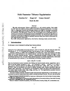
Figure 1: Mode-1, mode-2 and mode-3 unfoldings of a 3-way tensor χ. It is easy to visualize unfolding operations in terms of frontal, horizontal and lateral slices. The unfolding operation corresponds to aligning the corresponding slices for each mode next to each other. mode-l fibers are vectors in RNl that are obtained by varying the index in the lth dimension of the tensor and fixing the others [30]. As shown in Fig. 1, for 3-way tensors, we can visualize the unfolding operations in terms of frontal, horizontal and lateral slices. Although we do not give formal definitions for horizontal and lateral slices, which are obvious from Fig. 1, we denote the k th frontal face of a 3-way tensor χ by X(k) , as this notation will be useful. Folding and unfolding operators can be represented with permutation of lexicographically ordered vectors [20]. Specifically, the mode-l unfolding maps the tensor element (i1 , ⋯, iNK ) to the matrix element (il , j) according to [30] N

k−1

k=1 k≠l

m=1 m≠l

j = 1 + ∑ (ik − 1)Jk , where Jk = ∏ Nm .

(1)

Let us denote the vectorized form of χ by x and of χ(l) by xl . Then the relationship between x and xl is xl = Pl x and x = PT l xl , where Pl ∈ RN1 N2 ...NK ×N1 N2 ...NK is the permutation matrix that corresponds to the lth unfolding operation given by (1). Note that x and x1 are equal and P1 is the identity matrix. This notation will be useful in Section 5. To construct our second tensor nuclear norm regularization approach in Section 4.2 we need the t-SVD of [38] which in turn requires that we introduce three operators: fold, unfold and bcirc. While the mode-1 unfolding aligns frontal slices next to each other, the unfold(χ) operation aligns them on top of each

other:

⎡ X(1) ⎤ ⎢ ⎥ ⎢ X(2) ⎥ ⎢ ⎥ ⎥ unfold(χ) = ⎢ ⎢ ⋮ ⎥ ⎢ (N ) ⎥ ⎢X 3 ⎥ ⎣ ⎦

and fold(unfold(χ)) folds them back to a tensor form: fold(unfold(χ)) = χ. Using the X(k) ’s, one can form the block circulant matrix bcirc(χ) ∈ RN3 N1 ×N3 N2 as follows: ⎡ X(1) ⎢ ⎢ X(2) ⎢ bcirc(χ) = ⎢ ⎢ ⋮ ⎢ (N ) ⎢X 3 ⎣

X(N3 ) X(1) ⋱ X(N3 −1)

X(N3 −1) X(N3 ) ⋱ X(N3 −2)

⋯ ⋯ ⋱ ⋯

X(2) ⎤⎥ X(3) ⎥⎥ ⎥. ⋮ ⎥⎥ (1) ⎥ X ⎦

(2)

The n-mode product of a K-way tensor χ ∈ RN1 ×N2 ×⋯NK with matrix U ∈ R produces a tensor in with size N1 × ⋯ × Nn−1 × J × Nn+1 × ⋯ × NK and defined as J×Nn

Nn

(χ ×n U)i1 ⋯in−1 j in+1 ⋯iK = ∑ xi1 i2 ⋯iK ujin , in =1

where ×n is the n-mode product operation. While the n-mode product defines an operation between a tensor and a matrix, multiplication of 3-way tensors can be performed using the t-product [38]. For χ1 ∈ RN1 ×N2 ×N3 and χ2 ∈ RN2 ×`×N3 the t-product is given as χ1 ∗ χ2 = fold(bcirc(χ1 )unfold(χ2 )).

(3)

Notice that, χ1 ∗ χ2 is in RN1 ×`×N3 . The t-product defined in (3) is the basis for the t-SVD (tensor SVD) and the regularizer, TNN-2, which is introduced in Section 4.2. Given χ ∈ RN1 ×N2 ×N3 , its transpose, χT ∈ RN2 ×N1 ×N3 , is obtained by applying matrix transpose to each frontal face and then reversing the order of transposed frontal slices 2 through N3 : ⎡ (1) T ⎤ ⎛⎢⎢ (X ) ⎥⎥⎞ ⎜⎢(X(N3 ) )T ⎥⎟ ⎜⎢ ⎥⎟ T ⎢ ⎥⎟ . ⋮ χ = fold ⎜ ⎜⎢ ⎥⎟ ⎜⎢ (X(3) )T ⎥⎟ ⎜⎢ ⎥⎟ ⎝⎢⎢ (X(2) )T ⎥⎥⎠ ⎣ ⎦ The tensor Q is orthogonal in the sense of the t-product if QT ∗ Q = Q ∗ QT = I, where I is the identity tensor whose first frontal face is the ` × ` identity matrix, and whose other frontal slices are all zeros.

Figure 2: Parallel beam X-ray measurement geometry. We now review the block diagonalization property of block circulant matrices. For any block circulant matrix bcirc(χ) ∈ RN3 N1 ×N3 N2 we have (FN3 ⊗ IN1 ) ⋅ bcirc(χ) ⋅ (F∗N3 ⊗ IN2 ) ˆ (1) ⎡X ⎢ ⎢ ˆ (2) X ⎢ =⎢ ⎢ ⎢ ⎢ ⎣

⎤ ⎥ ⎥ ⎥ ⎥, ⎥ ⋱ ⎥ (N3 ) ⎥ ˆ X ⎦

(4)

where IN1 and IN2 are the identity matrices in RN1 ×N1 and RN2 ×N2 , respectively, FN3 ∈ RN3 ×N3 is the normalized discrete Fourier Transform matrix [43] and ˆ (n) ’s are the frontal faces of the tensor χ, X ˆ which is obtained by applying the Fast Fourier Transform (FFT) to the mode-3 fibers of χ. We will use this ˆ (n) for the tensor χ and its nth frontal face in the Fourier notation, ie., χ ˆ and X domain in Section 4.2. Finally, we note that bcirc(.) is a linear operation, which can be written in terms of permutation matrices. Let x denote the vectorized version of χ as described before, and let xc denote the vectorized version of bcirc(χ). Then, we have ⎡ Pc,1 ⎤ ⎢ ⎥ ⎢P ⎥ ⎢ c,2 ⎥ ⎥ x, x c = Pc x = ⎢ (5) ⎢ ⋮ ⎥ ⎢ ⎥ ⎢Pc,N3 ⎥ ⎣ ⎦ where Pc,i ’s reorder the elements of x according to the column blocks of (2).

3

The Measurement Model and The Multi-spectral Unknown as a Tensor

Polychromatic CT [4, 7, 44] is based on the projection model P (φ, t) = ∫ S(E) exp (− ∫

µ(r, E) dr) dE L(φ,t)

(6)

0.8 cotton wax nylon ethanol soap plexiglass rubber

μ (1/cm)

0.6

0.4

0.2

0.02

Figure 3: materials.

0.04

0.06 Energy (Mev)

0.08

Multi-spectral phantom and the attenuation curves for existing

where µ(r, E) is the energy dependent attenuation coefficient, S(E) is the source spectrum and (φ, t) parametrizes the x-ray path L(φ, t). In this work, we used parallel beam measurement geometry [45] as depicted in Fig. 2. Under the assumption of infinitesimal detector bin width (i.e., perfect energy resolution) the polychromatic projection given in (6) simplifies to a monochromatic one, where sk = S(E)δ(E −Ek ), resulting in the following model for the data corresponding to the k th bin: P (φ, t; k) =sk exp (− ∫

L(φ,t)

µ(r, Ek ) dr)

(7)

for k = 1, ..., N3 , where N3 is the number of energy bins. We refer the reader to [46] for an example of a fully polychromatic energy-resolved CT model. In order to obtain a discrete representation of (7), we discretize each µ(r, Ek ) into images of Np = N1 N2 pixels: xk ∈ RNp for k = 1, ..., N3 where N1 and N2 refers to the number of pixels in spatial dimensions x and y. We also discretize the (φ, t) space into Nm source detector pairs and introduce the system matrix A ∈ RNm ×Np where [A]ij represents the length of that segment of ray i passing through pixel j. Incorporating the Poisson statistics of X-ray interactions, the multi-energy measurement model is written yk,j = Poisson {sk exp [Axk ]j } ,

(8)

where k and j index detector bins and source-detector pairs respectively. Note that, the electronic noise can be neglected for PCDs, This is different than conventional CT where energy integrating detectors are used [13, 14]. Our goal is to develop an image formation method that treats all of the xk ’s in a unified manner, as done in [9], rather than reconstructing each independently of the others [12]. Towards this aim, we utilize tensors which are multi-linear generalizations of vectors and matrices. Specifically, we define the three-way (3rd -order) tensor χ ∈ RN1 ×N2 ×N3 , where first two are spatial dimensions the third dimension is energy, and the xk ’s are the lexicographical ordering

of the N1 × N2 frontal slices. A depiction of the multi-spectral phantom used in this study along with the corresponding attenuation curves are given in Figure 3. Note that the multi-linear structure can be extended to higher dimensions for different classes of problems. For example, one can consider a 5D dynamical problem with additional 3rd spatial dimension and time dependency. The goal of the multi-energy CT problem in this paper however is to reconstruct χ given yk,j for k = 1, ⋯, N3 and y = 1, ⋯, Nm .

4

Low-Rank modeling and Regularization

As mentioned before, low-rank modeling is an important tool not only for compressing [47] and analyzing [29, 48] large data sets but also for regularization and the incorporation of prior information [9, 49]. Traditionally, low-rank modeling is applied to a matrix variable, which is assumed to be low order or of low complexity [50]. As the multi-linear generalizations, such as our multi-spectral unknown in the form of a 3-way tensor, are closely related to the matrix case, we briefly describe the rank minimization problem of matrices in this section. Let the matrix X ∈ RN ×M denote the unknown variable that is assumed to be low-rank. For instance, X can be the system parameters of a low-order control system [50], a low dimensional representation of data [51], or adjacency ˆ with minimal matrix of a network graph [52]. The problem of estimating X rank from the output m of a system K can be formulated as a minimization problem: minimize rank(X) X∈RM ×N (9) subject to K(X) = m. However, minimization of rank(X), which is a non-convex function of X, is an NP-hard problem [32]. Consequently, Fazel et al. [50] proposed the replacement of the rank function with the nuclear norm, which is defined as min(M,N )

∥X∥∗ ∶=

∑

σi (X),

i

where σi ’s are the singular values of the matrix X. This replacement results in the following optimization problem. minimize

∥X∥∗

subject to

K(X) = m.

X∈RM ×N

(10)

The minimization problem (10) is motivated by the fact that the nuclear norm provides the tightest convex relaxation for the rank operation in matrices [19]. The replacement of rank with the nuclear norm is analogous to the use of the `1 norm as a proxy to the `0 semi-norm to achieve sparse signal reconstructions [53]. Analysis of this convex relaxation technique and the equivalence of (9) and (10)

Figure 4: Tucker decomposition of a 3-way tensor. The core tensor G controls the interactions between the modes and matrices that multiply the core tensor in each mode for compressed sensing are analyzed in [32]. In the sequel we interpret the nuclear norm term as a regularizer and seek solutions to problems in the form ˜ ∶= argmin ∥K(X) − m∥2 + γ∥X∥∗ . X 2

(11)

X∈RM ×N

where R∗ (X) = γ∥X∥∗ and γ is the regularization parameter. The low-rank assumptions and the nuclear norm heuristics have been generalized to the multi-linear case, i.e., to tensors, using the unfolding operations [21, 35]. Inspired by these works, we developed the tensor nuclear norm regularizer (TNN-1), which is introduced in Section 4-A. Additionally, we define a new tensor nuclear norm, where we exploit the T-SVD [38]. This new tensor nuclear norm and the regularizer (TNN-2) based on its definition are defined in Section 4.2. The common property of TNN-1 and TNN-2 is the fact that they can be formulated as a matrix nuclear norm minimization problem, which we shall explain next.

4.1

Tensor Rank and the Generalized Tensor Nuclear Norm Regularizer (TNN-1)

We start with the definition of Tucker decomposition, as the generalized tensor nuclear norm is related to it. The Tucker model [24, 30] is a multi-linear extension of SVD where a K-way tensor χ ∈ RN1 ×N2 ×⋯NK is decomposed into a core tensor G ∈ Rr1 ×r2 ×⋯rK , which controls the interactions between the modes and K matrices, which multiply the core tensor in each mode: χ = G ×1 A1 ×2 A2 ⋯AK−1 ×K AK . Here, columns of Al ∈ RNl ×rl can be considered as left singular vectors of model unfolding and rl for l = 1, ⋯, K is referred to as the n-rank2 . In the general Tucker model, the Al ’s need not be orthogonal. The special case of the Tucker 2 The CP decomposition can be seen as a special case of Tucker where, the core tensor is super-diagonal. Therefore, r1 = r2 = r3 = r where the tensor rank due to CP, r, needs to be known a priori [30].

60

60

80

50 60 40

30 20

σi

σi

σi

40

40

20 20

10 0

0

50

100

150

0

0

50

100

0

150

i

i

2

4

6

8

10

12

i

Figure 5: The unfoldings of χ and their singular values in log scale. First row: χ(1) , χ(2) and χ(3) . Second row: {σ(χ(1) )}i=1,⋯,N1 , {σ(χ(2) )}i=1,⋯,N2 and {σ(χ(3) )}i=1,⋯,N3 . model where Al ’s are orthogonal matrices is referred to as the Higher-OrderSingular-Value-Decomposition (HOSVD) [28]. The Tucker model can also be written in terms of unfoldings. For the three-way case we have χ(1) = A1 G(1) (A3 ⊗ A2 )T χ(2) = A2 G(2) (A3 ⊗ A1 )T

(12)

χ(3) = A3 G(3) (A2 ⊗ A1 ) , T

where ⊗ is the Kronecker product. Fig. 4 illustrates the Tucker decomposition for the 3-way case. The equations given in (12) and definition of n-rank shows that if a tensor is low rank in its lth mode (i.e., rl < min(Nl , ∏k′ ≠l Nk′ )), its unfolding in the same mode is a low rank matrix. Due to this connection, the matrix nuclear norm has been generalized to tensors by utilizing the unfolding operation in each mode in order to estimate low-rank tensors via a convex minimization problem [21, 33, 35]. The generalized tensor nuclear norm for a K-way tensor is given as [21, 35] ∥χ∥∗ ∶=

1 N ∑ ∥χ(k) ∥∗ N k=1

(13)

We refer the reader to [35] for a thorough discussion about the relation of (13) to Tucker decomposition and Shatten 1-norm of matrices. The low-rank tensor concept is quite relevant to the multi-energy CT problem. X-ray attenuation at neighboring energies are highly correlated. Therefore, for spectral CT, one expects the third unfolding, χ(3) to be low-rank [9]. However, structural redundancies can also be exploited by enforcing low-rank structure on the other two unfoldings. To this end, we use the more general

form of the tensor nuclear norm given in (13), which was proposed by Tomioka et al. [20] as a regularizer: 3

R∗ (χ) = ∑ γk ∥χ(k) ∥∗ ,

(14)

k=1

where γk ’s can be regarded as regularization parameters that tune the importance of each unfolding. A different parameter for each unfolding is assigned in order to make the regularizer more flexible [20], in a way that low-rank assumptions on any mode can be discarded if desired. For instance, see Section 7 for the examples where we set γ1 and γ2 to zero. Fig. 5 demonstrates the unfoldings of the phantom with 12 energy levels given in Fig. 3 and their singular values. The rapid decay of the singular values provides an indication of the usefulness of (14) as a regularizer for multi-energy CT reconstruction.

4.2

A t-SVD Based Tensor Nuclear Norm and Regularization (TNN-2)

In [38] it is shown that any tensor χ ∈ RN1 ×N2 ×N3 can be factored as χ = U ∗ S ∗ VT , where U ∈ RN1 ×N1 ×N3 and V ∈ RN2 ×N2 ×N3 are orthogonal, and S ∈ RN1 ×N2 ×N3 is made up with diagonal frontal faces. It is easy to show that, as is the case with the common matrix SVD, the t-SVD allows the tensor χ to be written as a finite sum of outer product of matrices [39]: χ=

min(N1 ,N2 )

∑

U(∶, i, ∶) ∗ S(i, i, ∶) ∗ V(∶, i, ∶)T ,

(15)

i=1

where (∶, i, ∶) and (∶, ∶, i) correspond to the ith lateral and ith frontal faces respectively, and (i, i, ∶) is the ith mode-3 fiber, similar to Matlab’s indexing. Now, we have the following relationship in the Fourier domain [38] (1) (1) ⎡χ ⎤ ⎡U ⎤ ⎢ˆ ⎥ ⎢ˆ ⎥ ⎢ ⎥ ⎢ ⎥ ⋱ ⋱ ⎢ ⎥=⎢ ⎥ ⎢ ⎥ ⎢ ⎥ (n) (N ) ˆ 3 ⎥ ⎢ ⎥ ⎢ χ ˆ U ⎣ ⎦ ⎣ ⎦ (1) (1) ⎤ ⎤T ⎡S ⎡ ˆ ⎢ˆ ⎥ ⎢V ⎥ ⎢ ⎥ ⎢ ⎥ ⋱ ⋱ ⎥⋅⎢ ⎥ , ⋅⎢ ⎢ ⎥ ⎢ ⎥ ˆ (N3 ) ⎥ ⎢ ˆ (N3 ) ⎥ ⎢ S V ⎣ ⎦ ⎣ ⎦

(16)

where the left-hand-side is the block diagonalized version of χ as given in (4) ˆ (n) = U ˆ (n) S ˆ (n) (V ˆ (n) )T is the SVD of the block, A ˆ (n) . In the light of (15) and A and (16) we propose the following tensor nuclear norm: ∥χ∥⊛ ∶=

min(N1 ,N2 ) N3

∑

ˆ i, j). ∑ S(i,

i=1

j=1

150

σi

100

50

0

0

500

1000

1500

i

Figure 6: The block circulant matrix bcirc(χ) and its singular values. Notice that we use the circled asterisk for this tensor nuclear norm definition. From (16) we have ∥χ∥⊛ = ∥(Fn ⊗ IN1 ) ⋅ bcirc(χ) ⋅ (F∗N3 ⊗ IN2 )∥∗ = ∥bcirc(χ)∥∗ ,

(17)

where the first follows immediately from (4) and the second line is due to the unitary invariance of the matrix nuclear norm. A consequence of (17) is that ∥.∥⊛ is a valid norm since i. For any tensor χ ∈ RN1 ×N2 ×N3 , ∥χ∥⊛ = ∥bcirc(χ)∥∗ ≥ 0, and when χ = 0, by definition ∥χ∥⊛ = ∥bcirc(χ)∥∗ = 0. ii. Let a ∈ R, then ∥aχ∥⊛ = ∥bcirc(aχ)∥∗ = ∥a(bcirc(χ))∥∗ = ∣a∣∥bcirc(χ)∥∗ = ∣a∣∥χ∥∗ iii. Let χ1 and χ2 be two tensors. ∥χ1 + χ2 ∥⊛ = ∥bcirc(χ2 + χ2 )∥∗ = ∥bcirc(χ1 ) + bcirc(χ2 )∥∗ ≤ ∥bcirc(χ1 )∥∗ + ∥bcirc(χ2 )∥∗ = ∥χ1 ∥⊛ + ∥χ2 ∥⊛ . Similar to the TNN-1 case, we use the new tensor nuclear norm given in (17) as a regularizer and form TNN-2 as: R⊛ = γ∥χ∥⊛ = γ∥bcirc(χ)∥∗ Fig. 6 demonstrates bcirc(χ) of the phantom given in Fig. 3 and its singular values, which rapidly decay. It has been shown that a truncated t-SVD representation provides an optimal representation in the same way that a truncated matrix SVD would give an optimal low rank approximation to the matrix in terms of the Frobenius norm [38]. Thus, our newly defined tensor nuclear norm, which is based on t-SVD, is more analogous to the matrix nuclear norm than generalized tensor nuclear norm given in (13) in this sense. Additionally, compared to TNN-1, TNN-2 has only one regularization parameter that needs to be determined.

5

Inverse Problem Formulation

The measurement model given in (8) leads to the penalized weighted least squares (PWLS) formulation [54] which gives quadratic approximation to the Poisson log-likelihood function for k th energy bin as Lk (xk ) = (Axk − mk )T Σ−1 i (Axk − mk ). −1 Here, [mk ]j = log(si /yk,j ) and Σ−1 k is a diagonal weighting matrix with [Σk ]jj = yk,j . Adding Lk ’s and the regularization function R(χ) we obtain a convex objective function:

minimize χ

1 N3 ∑ Lk (xk ) + R(χ), 2 k=1

(18)

where R(χ) is a combination of R∗ (χ) or R⊛ (χ) with a total variation (TV) regularizer. We have considered two types of TV regularizers. The first one, which is denoted by T V (χ), is the weighted superposition of isotropic TV operator (2D TV) applied to the frontal slices of χ as N3

T V (χ) ∶= ∑ αk T V (xk ) k=1 N3

(19)

N1 −1 N2 −1

∶= ∑ αk ∑ ∑ ∣(∇X(k) )i,j ∣ k=1

i=1

j=1

where (∇X(k) )i,j = [(∇x X(k) )i,j (∇y X(k) )i,j ]T with (∇x X(k) )i,j = Xi+1,j − Xi,j (k)

(k)

and (∇y X(k) )i,j = Xi,j+1 − Xi,j , (k)

(k)

Here, the αk ’s are the regularization parameters. The second one, which is denoted by T V3D (χ), is the three dimensional TV (3D TV) operator defined as N1 −1 N2 −1 N3 −1

T V3D (χ) ∶= α ∑ ∑ ∑ ∣(∇χ)i,j,k ∣ k=1

i=1

j=1

where (∇χ)i,j,k is the obvious extension of the 2D case to 3D. In the remainder of the paper we refer the first approach as TV and the second as 3D-TV regularization. TV regularization favors images with sparse gradients, hence it works well for piecewise constant image reconstruction. However, due its stair-casing effect TV tends to be problematic for texture recovery [55]. As we demonstrate empirically in Section 7, combining the tensor nuclear norm regularizer with TV reduces the amount of TV needed for reasonable noise cancellation and helps with recovering the texture.

6

Solution Algorithm via alternating direction method of multipliers (ADMM)

ADMM is a combination of dual decomposition and augmented Lagrangian methods [56, 57]. Although it results in a four-fold increase in the number of variables in the minimization procedure (see Section VI-A), ADMM provides a simple splitting scheme that breaks down a cost function, which is hard minimize, into pieces that are more tractable and can be minimized efficiently. Splitting based methods have been used for several problems including iterative CT reconstruction [58–60], image recovery [61] and restoration [62] and tensor completion [20, 21]. We examine the solution algorithm according to the structure of R(χ).

6.1

TNN-1 and TV Regularization

The first case is when R∗ (χ) is combined with T V (χ): R1 (χ) = R∗ (χ) + RT V (χ) First, the optimization problem given in (18) for R1 (χ) is reformulated as 3 1 N3 ∑ Lk (xk ) + ∑ γk ∥Zl ∥∗ + T V (χ) 2 k=1 l=1

minimize

χ,Z1 ,Z2 ,Z3

(20)

subject to Zl = χ(l) , for l = 1, 2, 3. To solve (20) we form the augmented Lagrangian as Lη (χ, {Zl }, {Yl }) =

3 1 N3 ∑ Lk (xk ) + ∑ γk ∥Zl ∥∗ 2 k=1 l=1 3

+ T V (χ) + ∑ ⟨Yl , χ(l) − Zl ⟩

(21)

l=1

+

η 3 2 ∑ ∥χ(l) − Zl ∥F , 2 k=l

where Yl ’s are dual variables, η > 0 is the penalty term and ⟨.⟩ is the inner product in the sense of Frobenius norm defined for K1 and K2 ∈ RM ×N as M N

⟨K1 , K2 ⟩ = ∑ ∑ [K1 ]ij ⋅ [K2 ]ij i=1 j=1

ADMM minimizes (21) for χ and Zk ’s in an alternating manner and then updates the dual variables: χn+1

∶= argmin Lη (χ, {Zl }n , {Yl }n ) ,

Zn+1 l

∶= argmin Lη (χn+1 , {Zl }, {Yl }n ) , for l = 1, 2, 3,

Yln+1

∶=

χ

Zl Yln + η(χn+1 (l)

− Zln+1 ), for l = 1, 2, 3.

(22)

Using the permutation matrix notation given in Section 2 we can write 3

3

l=1

l=1

T T ∑ ⟨Yl , χ(l) − Zl ⟩ = ∑ ⟨Pl yl , x − Pl zl ⟩ N3 3

T = ∑ ∑ ⟨{PT l yl }k , xk − {Pl zl }k ⟩ k=1 l=1

and 3

N3 3

l=1

k=1 l=1

2 T 2 ∑ ∥χ(l) − Zl ∥F = ∑ ∑ ∥xk − {Pl zl }k ∥ ,

where {.}k refers to the index set of corresponding energy (e.g., 1, ⋯, N3 for k = 1). Hence, the χ update in (22) can be decoupled and each xk can be treated separately: 3

T xn+1 ∶= argmin Lk (xk ) + ∑ ⟨{PT l yl }k , xk − {Pl zl }k ⟩ k xk

l=1 3

2 + ∑ ∥xk − {PT l zl }k ∥ + αk T V (xk ), l=1

which is a total variation regularized quadratic problem that can be solved using various methods [63, 64]. We used FISTA [65] in this work. With a straightforward reformulation one finds that the Zl updates can be obtained via the proximity operator of the nuclear norm as Zn+1 l

∶= argmin ∥Zl ∥∗ + Zl

∶= prox

γl η

Yln ∥.∥∗ ( η

η 2γl

∥

Yln η

+ χn+1 (l) ∥

∗

+ χn+1 (l) )

which has an analytical solution via the singular value shrinkage operator [18]. Specifically prox γl ∥.∥∗ (Z) = US γl (Σ)V T , (23) η

η

where Z = UΣV is the singular value decomposition of Z and Sρ(Σ) = diag({(σi − ρ)+ }) is the shrinkage operator with t+ = max(t, 0) applied to the singular values. T

6.2

TNN-2 and TV Regularization

Replacing TNN-1 with TNN-2 gives R2 (χ) = R⊛ (χ) + RT V (χ) and minimize χ,Z

1 N3 ∑ Lk (xk ) + γ∥Z∥∗ + T V (χ) 2 k=1

subject to Z = bcirc(χ).

(24)

needs to be solved. The augmented Lagrangian for (24) is given as Lη (χ, Z, Y) =

1 N3 ∑ Lk (xk ) + γ∥Z∥∗ 2 k=1

+ T V (χ) + ⟨Y, bcirc(χ) − Z⟩ η + ∥bcirc(χ) − Z∥2F , 2 In order to update xk ’s separately as in the TNN-1 case, using the definition of bcirc(.) operation given in (5), we can write N3

⟨Y, bcirc(χ) − Z⟩ = ∑ ⟨{y}k , xk − {z}k ⟩ k=1

and

N3

∥bcirc(χ) − Z∥2F = ∑ ∥xk − {z}k ∥2F k=1

where {.}k refers to the index set of k th energy (e.g., for k = 1 we have {[1, ⋯, N1 N2 ], [(N3 + 1)N1 N 2 + 1, ⋯, (N3 + 2)N1 N 2 + 1], ⋯, [(N32 − 1)N1 N2 + 1, ⋯, N32 N1 N2 ]}). Given this notation, we note that the solution algorithm of (24) is identical to the TNN-1 case described in Section VI-A. 0.35 0.6

0.3

0.5

0.25

0.4

0.2

0.3

0.15

0.2

0.1

0.1

0.05

0

0

Ground truth 25 keV

Ground truth 85 keV

Figure 7: Ground truth for Phantom-1. Left: 25 keV. Right: 85 keV In Section 7 we show examples where R(χ) = R∗ (χ), R(χ) = R⊛ (χ), R(χ) = RT V (χ) and R(χ) = RT V3D (χ). Solution to first two cases are straightforward variations where the latter case corresponds to reconstructing images for each energy independently using TV regularization. The last case results in a 3D linear inverse problem with TV regularization, for which we have used the UPN algorithm described in [66].

7

Reconstruction Examples

We compared the following methods in our simulations: 1. Filtered back projection (FBP) [67] algorithm applied to each energy bin separately. A RamLak filter multiplied with a Hamming window was used in the FBP inversion [67].

0.6 0.5 0.4 0.3 0.2 0.1 0

FBP

TNN-1

TNN-2

TV

3D-TV

TNN-1+TV

0.6 0.5 0.4 0.3 0.2 0.1 0

TNN-2+TV

Figure 8: Phantom-1: Reconstructions results for 25 keV. 0.35 0.3 0.25 0.2 0.15 0.1 0.05 0

FBP

TNN-1

TNN-2

TV

3D-TV

TNN-1+TV

0.35 0.3 0.25 0.2 0.15 0.1 0.05 0

TNN-2+TV

Figure 9: Phantom-1: Reconstructions results for 85 keV. 2. Only TV regularization at each energy bin separately (i.e., λnuc = 0 in (18)). 2. 3D-TV regularization. 4. Only TNN-1 regularization (i.e., αk = 0 for k = 1, ⋯, N3 in (19). 5. Only TNN-2 regularization. 6. TNN-1 and TV regularization.

Table 1: Error performance with respect to FBP: Elapsed times at particular iterations when FBP is outperformed for each method. The 3D-TV method uses an optimized C code that is called from Matlab [66]. All other methods use a non-optimized Matlab code. Method E`2 (25keV) Iteration Number Comp. time (sec) FBP 0.2010 4 TNN-1 0.1401 2 1.25 TNN-2 0.1837 3 8.2 TV 0.1919 17 24.66 3D-TV 0.1376 1 0.15 TV+TNN-1 0.1093 1 165 TV+TNN-2 0.1526 2 342 7. TNN-2 and TV regularization. 9. TNN-1 with γ1 and γ2 are set to 0. Quantitative accuracy of the reconstructions were determined by relative `2 error, E`2 which is given as E`2 =

∥ˆ xk − x∗k ∥22 . ∥x∗k ∥22

ˆ k and x∗k are the reconstruction and the true images at the kth energy Here, x respectively, and ∥ ⋅ ∥ is the Euclidean norm. We simulated multi-spectral data for 12 energies between 25 and 85 keV for 16 uniformly distributed angles between 0 and 180 degrees. We chose 25-85 keV range as it covers the lower portion of the X-ray source spectra of 20-140 keV used in CT [45], where materials are better differentiated (see Fig. 3). We assumed the X-ray spectra is uniform with 106 photons at each energy. We have used 2 different phantoms in our experiments. In addition to the piecewise constant phantom (128x128 pixels) shown in Fig. 3 and 7, which we call Phantom-1, we generated another phantom with isotropic texture on the objects and with a small linear variation to the background for more realistic experiments. This second phantom is called Phantom-2 and is shown in see Fig. 11. To explore the performance of the approach using a more realistic phantom we employed a DICOM image obtained from a CT scan of a duffel bag and artificially assigned attenuation values that are in the same range as Phantom-1 (see Fig. 14). For all cases considered here, simulations are performed in MATLAB [68] except for the 3D-TV implementation we have used the code available at http://www2.imm.dtu.dk/∼pcha/TVReg/, which is written in C. We have used a 8 core Intel CPU with 16 gigabytes of memory. Note that the code we have used for these experiments is written in Matlab and is in no sense optimized for efficiencies which could be obtained using a lower level language and exploiting parallel architectures. Indeed, the bulk of the computation time comes from the projection and back-projection operations (i.e.,

0.35

0.3

Reconstrution Error

0.25 FBP Level

TNN−2 TNN−1 FBP 3D−TV TNN2−TV TNN1−TV TV

0.2

0.15

0.1

0.05

0

0

20

40

60

80

100

Iteration

Figure 10: Relative E`2 error versus iteration number for 85keV results from Phantom-1. The horizontal line represents the error level achieved by FBP. Note that all methods are implemented in Matlab except for 3D-TV which is written in C. A, AT ) and from the computation singular values, both of which can be performed efficiently using fast and parallel algorithms [69, 70] in order to achieve a real-time reconstruction algorithm, which is crucial for the baggage inspection application. In order to implement the singular value soft thresholding operation given in (23), we used the PCA (principle component analysis) [43] algorithm given in [71], which returns a rank k approximation of a n × m matrix in O(mn log k + l2 (m + n)) operations, where l is an integer bigger than and close to k. Hence, we avoided the explicit calculation of SVD at each iteration, which can be calculated in O(knm) operations using a standard QR decomposition based algorithm [43].The linear attenuation values for the materials in Phantom-1 are taken from XCOM: Photon cross sections database [72]. 1 0.25 0.8 0.2 0.6 0.4

0.15 0.1

0.2

0.05

0

0

Ground truth 25 keV

Ground truth 85 keV

Figure 11: Ground truth for Phantom-2. Left: 25 keV. Right: 85 keV

In all examples we set η, γ1 , γ2 , γ3 = 0.4 and γ = 0.1. We let αi ’s reduce from 0.05 to 0.03 in a quadratic manner from k = 1, ⋯, N3 as low energy images need stronger regularization due to the higher level of Poisson noise. The 3DTV regularization parameter α was set to 0.1. We tuned the regularization parameters manually and used the same set of parameters for both phantoms, as they gave the best error performance. We emphasize that systematic selection of regularization parameters is an important problem, which continues to be an active area of research, especially for non-quadratic regularization techniques such as TV and nuclear norm regularization [73–75]. 1 0.8 0.6 0.4 0.2 0

FBP

TNN-1

TNN-2

TV

3D-TV

TNN-1+TV

1 0.8 0.6 0.4 0.2 0

TNN-2+TV

Figure 12: Phantom-2: Reconstructions results for 25 keV. We show the error performance vs. iteration number for each method for 85keV and Phantom-1 in Fig. 10. We display the reconstructions for the 25 keV and 85 keV bins as representatives of high and low regions of the spectra. Fig. 8, Fig. 12 and Fig. 15 show reconstruction results for 25 keV images; Fig. 9, Fig. 13 and Fig. 16 show reconstruction results for 85 keV images for both phantoms. Table 1 gives the elapsed times at particular iterations when FBP is outperformed for each method. Table 2, Table 3 and Table 4 give quantitative error performance as well as the computation times. Firstly, we observe that pure FBP fails to provide reasonable reconstructions at low energies due to limited number of views and noise.The proposed methods outperformed FBP in at most 3 iterations for 85keV and Phantom-1. Second, when TNN-1 or TNN-2 is used as the only regularizer, they provide considerable noise reduction while preserving much of the detail. Additionally, as seen in Table 2 they allow rapid processing relative to the other methods considered here. When they are combined with TV, TNN-1 and TNN-2 regularizers enhance its detail preserving capabilities and increases the reconstruction quality of low energy at the price of increased computational burden, which can be observed

0.25 0.2 0.15 0.1 0.05 0

FBP

TNN-1

TNN-2

TV

3D-TV

TNN-1+TV

0.25 0.2 0.15 0.1 0.05 0

TNN-2+TV

Figure 13: Phantom-2: Reconstructions results for 85 keV. 0.35

1

0.3 0.8

0.25 0.2

0.6

0.15

0.4

0.1 0.2

0.05

0

0

Ground truth 25 keV

Ground truth 85 keV

Figure 14: Ground truth for Phantom-3. Left: 25 keV. Right: 85 keV especially in the examples with Phantom-2. Although 3D-TV outperforms TV as it incorporates the smoothness in the energy dimension, TNN-1 and TNN-2 combined with TV gives superior results. Finally, we observe that TNN-1 and TNN-2 perform similarly in terms of image quality when they are the only regularizers that are used. However, for the 85 keV images we see that when combined with TV, TNN-2 outperforms TNN-1. In the last example, we demonstrate the efficiency of the tensor model in constructing a regularizer based on low-rank assumptions. We consider using the TNN-1 regularizer with γ1 and γ2 are set to 0. This is equivalent to applying the low rank prior to the multi-spectral matrix whose columns are vectorized images at different energies. In addition to the data set with 12 energy bins, we simulated data for 25 bins uniformly distributed between the same range of 25 keV and 85 keV with Phantom-1. All other parameters were kept the same. Fig. 17, Fig. 18 and Table 5 shows the results for both data sets. We observe that that the tensor-based representation is needed to design useful nuclear norm

1 0.8 0.6 0.4 0.2 0

FBP

TNN-1

TNN-2

TV

3D-TV

TNN-1+TV

1 0.8 0.6 0.4 0.2 0

TNN-2+TV

Figure 15: Phantom-3: Reconstructions results for 25 keV. 0.35 0.3 0.25 0.2 0.15 0.1 0.05 0

FBP

TNN-1

TNN-2

TV

3D-TV

TNN-1+TV

0.35 0.3 0.25 0.2 0.15 0.1 0.05 0

TNN-2+TV

Figure 16: Phantom-3: Reconstructions results for 85 keV. regularization with the TNN-1 approach. Although increasing the number of bins from 12 to 25 introduces more redundancy in the energy dimension, the incorporation of the unfoldings in the spatial dimensions is still essential.

8

Conclusions

In this paper, we provided an algorithmic framework for iterative multi-energy CT and showed that generalized tensor nuclear norm ideas can be used as reg-

Table 2: Error performance of different methods for Phantom-1 Method E`2 (25keV) E`2 (85keV) Comp. time (sec) FBP 0.4507 0.2010 4 TNN-1 0.0492 0.0335 25 TNN-2 0.0299 0.0215 112 TV 0.0149 0.0101 249 3D-TV 0.0078 0.0118 196 TV+TNN-1 0.0056 0.0122 3615 TV+TNN-2 0.0066 0.0045 10879

Table 3: Error performance of different methods for Phantom-2 Method E`2 (25keV) E`2 (85keV) Comp. time (sec) FBP 0.2102 0.1845 4 TNN-1 0.0583 0.0492 28 TNN-2 0.0598 0.0514 140 TV 0.0465 0.0202 284 3D-TV 0.0140 0.0185 162 TV+TNN-1 0.0093 0.0175 3911 TV+TNN-2 0.0096 0.0102 11470

Table 4: Error performance of different methods for Phantom-3 Method E`2 (25keV) E`2 (85keV) Comp. time (sec) FBP 0.6216 0.3482 4 TNN-1 0.1632 0.1057 18 TNN-2 0.1634 0.1124 51 TV 0.1482 0.0879 203 3D-TV 0.1553 0.1028 112 TV+TNN-1 0.1365 0.0881 2891 TV+TNN-2 0.1395 0.0886 5570

Table 5: Error performance of the different unfolding trials with Phantom-1 Method E`2 (20keV) E`2 (85keV) Comp. time (sec) TNN 0.0341 0.0335 25 TNN, γ1,2 = 0 0.0708 0.0694 25 TNN 25 bins 0.0327 0.0314 64 TNN, 25 bins γ1,2 = 0 0.0713 0.0693 72

0.6 0.5 0.4 0.3 0.2 0.1 0

TNN-1,γ1,2 = 0

TNN-1,γ1,2 = 0

TNN-1

25 Bins

TNN-1

25 Bins

Figure 17: Phantom-1: Reconstructions results for 20 keV with TNN-1 where γ1 and γ2 are set to 0. 0.35 0.3 0.25 0.2 0.15 0.1 0.05 0

TNN-1,γ1,2 = 0

TNN-1,γ1,2 = 0

25 Bins

TNN-1

TNN-1

25 Bins

Figure 18: Phantom-1: Reconstructions results for 85 keV with TNN-1 where γ1 and γ2 are set to 0. ularizers. Additionally we proposed an alternative tensor nuclear norm based on t-SVD and a regularizer based on this new tensor nuclear norm. The ideas presented here can be extended to any type of inverse problem where a multilinear description of the unknown is possible. Additionally, the tensor nuclear norm regularization can be generalized to higher dimensions. For instance, one can consider a the 5D problem with an additional spatial dimension and time dependency. In future, incorporation of low rank-sparse decomposition approaches [9, 76] in the tensor-based framework will be investigated. The applicability of Tucker and CANDECOMP/PARAFAC decomposition techniques especially to reduce the dimension of the multi-energy data cube will also be considered. These directions will allow the design of more sophisticated tensor nuclear norm regularizers. Another important extension is to design an algorithm to estimate the redundancy along different dimensions, which will allow us to quantify the requirement of low rank priors. As the goal of the multi-energy tomography problem is to reconstruct structurally similar images of the X-ray attenuation at each energy, it is sensible to design Tikhonov type, fast regularization techniques that explicitly enforce structural similarity. Design of such alternative regularizers is important especially for medical imaging applications considering the cartooning effect of TV

regularization. Development of an automatic determination of the regularization parameters is also an important future direction to increase the practicality of the algorithms presented. Considerable reduction of computation time is required in order to be able to use our methods in practice. Therefore, an important area of future work should be devoted to increasing the efficiency of implementation by,e.g., parallel computing and code optimization. Finally, the algorithms should be tested for real-life scenarios with experimental data and higher resolution reconstructions.

References [1] B. Whiting, P. Massoumzadeh, O. Earl, J. OSullivan, D. Snyder, and J. Williamson, “Properties of preprocessed sinogram data in x-ray computed tomography,” Medical physics, vol. 33, p. 3290, 2006. [2] C. Bouman and K. Sauer, “A unified approach to statistical tomography using coordinate descent optimization,” Image Processing, IEEE Transactions on, vol. 5, no. 3, pp. 480–492, mar 1996. [3] X. Pan, E. Sidky, and M. Vannier, “Why do commercial ct scanners still employ traditional, filtered back-projection for image reconstruction?” Inverse problems, vol. 25, p. 123009, 2009. [4] I. Elbakri and J. Fessler, “Statistical image reconstruction for polyenergetic x-ray computed tomography,” Medical Imaging, IEEE Transactions on, vol. 21, no. 2, pp. 89–99, 2002. [5] O. Semerci and E. Miller, “A parametric level-set approach to simultaneous object identification and background reconstruction for dual-energy computed tomography,” Image Processing, IEEE Transactions on, vol. 21, no. 5, pp. 2719 –2734, may 2012. [6] G. Wang, H. Yu, and B. De Man, “An outlook on x-ray ct research and development,” Medical physics, vol. 35, p. 1051, 2008. [7] B. De Man, J. Nuyts, P. Dupont, G. Marchal, and P. Suetens, “An iterative maximum-likelihood polychromatic algorithm for ct,” Medical Imaging, IEEE Transactions on, vol. 20, no. 10, pp. 999–1008, 2001. [8] P. Shikhaliev, “Energy-resolved computed tomography: first experimental results,” Physics in medicine and biology, vol. 53, p. 5595, 2008. [9] H. Gao, H. Yu, S. Osher, and G. Wang, “Multi-energy ct based on a prior rank, intensity and sparsity model (prism),” Inverse problems, vol. 27, p. 115012, 2011. [10] P. Shikhaliev and S. Fritz, “Photon counting spectral ct versus conventional ct: comparative evaluation for breast imaging application,” Physics in medicine and biology, vol. 56, p. 1905, 2011.

[11] J. Schlomka, E. Roessl, R. Dorscheid, S. Dill, G. Martens, T. Istel, C. B¨ aumer, C. Herrmann, R. Steadman, G. Zeitler et al., “Experimental feasibility of multi-energy photon-counting k-edge imaging in pre-clinical computed tomography,” Physics in medicine and biology, vol. 53, p. 4031, 2008. [12] V. Ivakhnenko, “A novel quasi-linearization method for ct image reconstruction in scanners with a multi-energy detector system,” Nuclear Science, IEEE Transactions on, vol. 57, no. 2, pp. 870–879, 2010. [13] J. Iwanczyk, E. Nygard, O. Meirav, J. Arenson, W. Barber, N. Hartsough, N. Malakhov, and J. Wessel, “Photon counting energy dispersive detector arrays for x-ray imaging,” Nuclear Science, IEEE Transactions on, vol. 56, no. 3, pp. 535–542, 2009. [14] W. Barber, E. Nygard, J. Iwanczyk, M. Zhang, E. Frey, B. Tsui, J. Wessel, N. Malakhov, G. Wawrzyniak, N. Hartsough et al., “Characterization of a novel photon counting detector for clinical ct: count rate, energy resolution, and noise performance,” in Proceedings of the SPIE Medical Imaging Conference, vol. 7258, 2009, p. 725824. [15] Z. Ying, R. Naidu, and C. Crawford, “Dual energy computed tomography for explosive detection,” J. of X-ray Sci. and Tech., vol. 14, no. 4, pp. 235–256, 2006. [16] S. Singh and M. Singh, “Explosives detection systems (EDS) for aviation security,” Signal Processing, vol. 83, no. 1, pp. 31–55, 2003. [17] E. Candes, X. Li, Y. Ma, and J. Wright, “Robust principal component analysis?” Arxiv preprint arXiv:0912.3599, 2009. [18] J. Cai, E. Candes, and Z. Shen, “A singular value thresholding algorithm for matrix completion,” Arxiv preprint arXiv:0810.3286, 2008. [19] E. Cand`es and B. Recht, “Exact matrix completion via convex optimization,” Foundations of Computational Mathematics, vol. 9, no. 6, pp. 717– 772, 2009. [20] R. Tomioka, K. Hayashi, and H. Kashima, “Estimation of low-rank tensors via convex optimization,” Arxiv preprint arXiv:1010.0789, 2010. [21] J. Liu, P. Musialski, P. Wonka, and J. Ye, “Tensor completion for estimating missing values in visual data,” in Computer Vision, 2009 IEEE 12th International Conference on. IEEE, 2009, pp. 2114–2121. [22] J. Cai, X. Jia, H. Gao, S. Jiang, Z. Shen, and H. Zhao, “Cine cone beam ct reconstruction using low-rank matrix factorization: algorithm and a proofof-princple study,” Arxiv preprint arXiv:1204.3595, 2012.

[23] J. Carroll and J. Chang, “Analysis of individual differences in multidimensional scaling via an n-way generalization of eckart-young decomposition,” Psychometrika, vol. 35, no. 3, pp. 283–319, 1970. [24] L. Tucker, “Some mathematical notes on three-mode factor analysis,” Psychometrika, vol. 31, no. 3, pp. 279–311, 1966. [25] E. Acar and B. Yener, “Unsupervised multiway data analysis: A literature survey,” Knowledge and Data Engineering, IEEE Transactions on, vol. 21, no. 1, pp. 6–20, 2009. [26] C. Andersen and R. Bro, “Practical aspects of parafac modeling of fluorescence excitation-emission data,” Journal of Chemometrics, vol. 17, no. 4, pp. 200–215, 2003. [27] T. Kolda and J. Sun, “Scalable tensor decompositions for multi-aspect data mining,” in Data Mining, 2008. ICDM’08. Eighth IEEE International Conference on. IEEE, 2008, pp. 363–372. [28] L. De Lathauwer, B. De Moor, and J. Vandewalle, “A multilinear singular value decomposition,” SIAM Journal on Matrix Analysis and Applications, vol. 21, no. 4, pp. 1253–1278, 2000. [29] M. Vasilescu and D. Terzopoulos, “Multilinear image analysis for facial recognition,” in Pattern Recognition, 2002. Proceedings. 16th International Conference on, vol. 2. IEEE, 2002, pp. 511–514. [30] T. Kolda and B. Bader, “Tensor decompositions and applications,” SIAM review, vol. 51, no. 3, p. 455, 2009. [31] R. Bro and H. Kiers, “A new efficient method for determining the number of components in parafac models,” Journal of Chemometrics, vol. 17, no. 5, pp. 274–286, 2003. [32] B. Recht, M. Fazel, and P. Parrilo, “Guaranteed minimum-rank solutions of linear matrix equations via nuclear norm minimization,” SIAM review, vol. 52, no. 3, pp. 471–501, 2010. [33] S. Gandy, B. Recht, and I. Yamada, “Tensor completion and low-n-rank tensor recovery via convex optimization,” Inverse Problems, vol. 27, p. 025010, 2011. [34] M. Signoretto, R. Van de Plas, B. De Moor, and J. Suykens, “Tensor versus matrix completion: a comparison with application to spectral data,” IEEE Signal Processing Letters, vol. 18, no. 7, p. 403, 2011. [35] M. Signoretto, L. De Lathauwer, and J. Suykens, “Nuclear norms for tensors and their use for convex multilinear estimation,” Technical Report 10-186, ESAT-SISTA, K.U.Leuven, 2010.

[36] M. Signoretto, Q. Dinh, L. De Lathauwer, and J. Suykens, “Learning with tensors: a framework based on convex optimization and spectral regularization,” Internal Report 11-129, ESATSISTA, KU Leuven (Leuven, Belgium), Tech. Rep., 2011. [37] O. Semerci, N. Hao, M. E. Kilmer, and E. L. Miller, “An iterative reconstruction method for spectral CT with tensor-based formulation and nuclear norm regularization,” in Proc. 2nd Intl. Mtg. on image formation in X-ray CT, 2012, pp. 314–7. [38] M. E. Kilmer and C. D. Martin, “Factorization strategies for third-order tensors,” Linear Algebra and its Applications, vol. 435, no. 3, pp. 641 – 658, 2011, ¡ce:title¿Special Issue: Dedication to Pete Stewart on the occasion of his 70th birthday¡/ce:title¿. [Online]. Available: http://www. sciencedirect.com/science/article/pii/S0024379510004830 [39] M. KILMER, K. BRAMAN, N. HAO, and R. Hoover, “Third order tensors as operators on matrices: a theoretical and computational framework with applications in imaging,” Department of Computer Science, Tufts University, 2011. [40] L. Rudin, S. Osher, and E. Fatemi, “Nonlinear total variation based noise removal algorithms,” Physica D: Nonlinear Phenomena, vol. 60, no. 1, pp. 259–268, 1992. [41] E. Sidky and X. Pan, “Image reconstruction in circular cone-beam computed tomography by constrained, total-variation minimization,” Physics in medicine and biology, vol. 53, p. 4777, 2008. [42] J. Tang, B. Nett, and G. Chen, “Performance comparison between total variation (tv)-based compressed sensing and statistical iterative reconstruction algorithms,” Physics in Medicine and Biology, vol. 54, p. 5781, 2009. [43] G. Golub and C. Van Loan, Matrix computations. Johns Hopkins University Press, 1996, vol. 3. [44] O. Semerci and E. Miller, “Tomographic imaging-a parametric level-set approach to simultaneous object identification and background reconstruction for dual-energy computed tomography,” IEEE Transactions on Image Processing, vol. 21, no. 5, p. 2719, 2012. [45] J. Beutel, Handbook of medical imaging: Physics and psychophysics. Spie Press, 2000, vol. 1. [46] T. Schmidt, “An empirical method for correcting the detector spectral response in energy-resolved ct,” in Proceedings of SPIE, vol. 8313, 2012, p. 831312. [47] J. Ye, “Generalized low rank approximations of matrices,” Machine Learning, vol. 61, no. 1, pp. 167–191, 2005.

[48] I. Jolliffe, Principal component analysis.

Wiley Online Library, 2005.

[49] S. Lefkimmiatis, J. Ward, and M. Unser, “A hessian schatten-norm regularization approach for solving linear inverse problems,” arXiv preprint arXiv:1209.3318, 2012. [50] M. Fazel, H. Hindi, and S. Boyd, “A rank minimization heuristic with application to minimum order system approximation,” in American Control Conference, 2001. Proceedings of the 2001, vol. 6. IEEE, 2001, pp. 4734– 4739. [51] M. Turk and A. Pentland, “Face recognition using eigenfaces,” in Computer Vision and Pattern Recognition, 1991. Proceedings CVPR’91., IEEE Computer Society Conference on. IEEE, 1991, pp. 586–591. [52] C. Hsieh, K. Chiang, and I. Dhillon, “Low rank modeling of signed networks,” in Proceedings of the 18th ACM SIGKDD international conference on Knowledge discovery and data mining. ACM, 2012, pp. 507–515. [53] D. Donoho, “Compressed sensing,” Information Theory, IEEE Transactions on, vol. 52, no. 4, pp. 1289–1306, 2006. [54] K. Sauer and C. Bouman, “A local update strategy for iterative reconstruction from projections,” Signal Processing, IEEE Transactions on, vol. 41, no. 2, pp. 534–548, 1993. [55] M. Elad, J. Starck, P. Querre, and D. Donoho, “Simultaneous cartoon and texture image inpainting using morphological component analysis (mca),” Applied and Computational Harmonic Analysis, vol. 19, no. 3, pp. 340–358, 2005. [56] S. Boyd, N. Parikh, E. Chu, B. Peleato, and J. Eckstein, Distributed optimization and statistical learning via the alternating direction method of multipliers. Now Publishers, 2011. [57] D. Bertsekas, “Nonlinear programming,” 1999. [58] Q. Xu, X. Mou, G. Wang, J. Sieren, E. A. Hoffman, and H. Yu, “Statistical interior tomography,” Medical Imaging, IEEE Transactions on, vol. 30, no. 5, pp. 1116–1128, 2011. [59] S. Ramani and J. A. Fessler, “A splitting-based iterative algorithm for accelerated statistical x-ray ct reconstruction,” Medical Imaging, IEEE Transactions on, vol. 31, no. 3, pp. 677–688, 2012. [60] B. Vandeghinste, B. Goossens, J. De Beenhouwer, A. Pizurica, W. Philips, S. Vandenberghe, and S. Staelens, “Split-bregman-based sparse-view ct reconstruction,” in 11th International meeting on Fully Three-Dimensional Image Reconstruction in Radiology and Nuclear Medicine (Fully 3D 11), 2011, pp. 431–434.

[61] M. V. Afonso, J. M. Bioucas-Dias, and M. A. Figueiredo, “Fast image recovery using variable splitting and constrained optimization,” Image Processing, IEEE Transactions on, vol. 19, no. 9, pp. 2345–2356, 2010. [62] M. A. Figueiredo and J. M. Bioucas-Dias, “Restoration of poissonian images using alternating direction optimization,” Image Processing, IEEE Transactions on, vol. 19, no. 12, pp. 3133–3145, 2010. [63] A. Chambolle, “An algorithm for total variation minimization and applications,” Journal of Mathematical imaging and vision, vol. 20, no. 1, pp. 89–97, 2004. [64] C. Vogel and M. Oman, “Fast, robust total variation-based reconstruction of noisy, blurred images,” Image Processing, IEEE Transactions on, vol. 7, no. 6, pp. 813–824, 1998. [65] A. Beck and M. Teboulle, “A fast iterative shrinkage-thresholding algorithm for linear inverse problems,” SIAM Journal on Imaging Sciences, vol. 2, no. 1, pp. 183–202, 2009. [66] T. L. Jensen, J. H. Jørgensen, P. C. Hansen, and S. H. Jensen, “Implementation of an optimal first-order method for strongly convex total variation regularization,” BIT Numerical Mathematics, vol. 52, no. 2, pp. 329–356, 2012. [67] M. Slaney and A. Kak, “Principles of computerized tomographic imaging,” SIAM, Philadelphia, 1988. [68] M. Guide, “The mathworks inc,” Natick, MA, vol. 4, 1998. [69] B. De Man and S. Basu, “Distance-driven projection and backprojection in three dimensions,” Physics in medicine and biology, vol. 49, no. 11, p. 2463, 2004. [70] M. Andrecut, “Parallel gpu implementation of iterative pca algorithms,” Journal of Computational Biology, vol. 16, no. 11, pp. 1593–1599, 2009. [71] F. Woolfe, E. Liberty, V. Rokhlin, and M. Tygert, “A fast randomized algorithm for the approximation of matrices,” Applied and Computational Harmonic Analysis, vol. 25, no. 3, pp. 335–366, 2008. [72] M. Berger, J. Hubbell, S. Seltzer, J. Chang, J. Coursey, R. Sukumar, and D. Zucker, “Xcom: Photon cross sections database,” NIST Standard Reference Database, vol. 8, pp. 87–3597, 1998. [73] S. Ahn and R. Leahy, “Analysis of resolution and noise properties of nonquadratically regularized image reconstruction methods for pet,” Medical Imaging, IEEE Transactions on, vol. 27, no. 3, pp. 413–424, 2008.

[74] S. Ramani, Z. Liu, J. Rosen, J. Nielsen, and J. Fessler, “Regularization parameter selection for nonlinear iterative image restoration and mri reconstruction using gcv and sure-based methods,” Image Processing, IEEE Transactions on, vol. 21, no. 8, pp. 3659–3672, 2012. [75] E. Candes, C. Sing-Long, and J. Trzasko, “Unbiased risk estimates for singular value thresholding and spectral estimators,” arXiv preprint arXiv:1210.4139, 2012. [76] M. Golbabaee and P. Vandergheynst, “Hyperspectral image compressed sensing via low-rank and joint-sparse matrix recovery,” in Indernational Conference on Acoustics, Speech and Signal Processing ICASSP, 2011.